A numerical investigation of constant-volume non-Boussinesq density currents

To cite this version : Bonometti, Thomas and Ungarish, Marius and Balachandar,

S. A numerical investigation of constant-volume non-Boussinesq density

currents. (2010) In: 7th International Conference on Multiphase Flow - ICFM 2010,

30 May 2010 - 04 June 2010 (Tampa, United States).

O

pen

A

rchive

T

OULOUSE

A

rchive

O

uverte (

OATAO

)

OATAO is an open access repository that collects the work of Toulouse researchers and

makes it freely available over the web where possible.

This is an author-deposited version published in :

http://oatao.univ-toulouse.fr/

Eprints ID : 10219

Any correspondance concerning this service should be sent to the repository

administrator: staff-oatao@listes-diff.inp-toulouse.fr

A numerical investigation of constant-volume non-Boussinesq density currents

Bonometti Thomas*, Ungarish

Marius'~~, Balachandar

s.t

*

Université de Toulouse, INPT, UPS, CNRS, Institut de Mécanique des Fluides de Toulouse, Allée Camille Soula, F-31400 Toulouse, France

'II Department of Computer Science, Technion, Haifa, 32000, Israel

tnepartment ofMechanical andAerospace Engineering, University ofFlorida, Gainesville FL32611, USA thomas.bonometti@imft.fr, unga@cs.technion.ac.il, bala1s@ufl.edu

Keywords: Density current, non-Boussinesq effects, Navier-Stokes simulation, shallow-water theory

Abstract

The time-dependent behaviour of non-Boussinesq high-Reynolds-number density currents of density Pc• released from a lock of height h0 and length

x

0 into a ambient of height H and density Pa• is considered. We use two-dimensional

Navier-Stokes simulations to cover a wide range of density ratio pcfpa (for both "heavy"-bottom and "light"-top currents) and geometrie ratios (H*=Hih0, Â=xofh0). To our knowledge, the ranges of parameters and times of propagation considered here

were not covered in previous experimental or numerical studies. In the frrst part, we set the lock aspect ratio to Â=18.75, and vary the density ratio 104<pcfpa<104 and initial depth ratio 1gl:5:50. The Navier-Stokes results are compared with predictions of a shallow-water model, in the regime of constant-speed (slumping) phase. Good agreement is observed in a large region of the parameter space (pcfpa; H*). The larger discrepancy is observed in the range of high-H* and low-pcfpa for which the shallow-water model overpredicts the velocity of the current. Two possible reasons are suspected, namely the fluid motion in the ambient fluid which is not accounted for in the model, and the choice of the model for the front condition. In the second part, we set the initial depth ratio to H*=lO, and vary the density ratio 10"2<pcfpa<102 and lock aspect ratio 0.5:5:). :5:18.75. In particular, we derive novel insights on the influence of the lock aspect ratio Â=xofho on the shape and motion of the current in the slumping stage. lt is shown that a critical value exists, Â,;,;1; the dynamics of the current is significantl y influenced by À if below

Âcnt· We present a simple analytical model which support the observation that for a light current the speed of propagation is

proportional to Â114 when Â<Âcnt·

Introduction

Constant-volume density currents have been studied extensive! y because of their importance in various industrial and environmental problems (e.g. Simpson 1982, Ungarish 2009). Horizontal density currents are buoyancy-driven flows which manifest themselves as a current of heavy (resp. light) fluid running below light (resp. above heavy) fluid. Initially after release the current accelerates and reaches a constant speed of spreading (referred to as the slumping phase, Huppert & Simpson 1980). This phase lasts until the backward propagating disturbance reflects off the back wall or symmetry plane and propagates forward to catch up with the front (Rottman & Simpson 1983). The duration of the slumping phase depends on the Reynolds number and volume of release. After the slumping phase, the current velocity decreases in a self-similar manner at a rate that depends on the dominant effect (inertia, viscosity, surface tension).

In the Boussinesq limit, the dynamics of planar currents of arbitrary initial depth ratios is relatively well understood thanks to various laboratory experiments (e.g.

Rotrnann & Simpson 1983; Marino, Thomas & Linden 2005), numerical investigations (Hlirtel, Meiburg & Necker 2000; Ozgokmen et al. 2004; Cantero et al. 2007, Ooi,

Constantinescu & Weber 2009) and analytical modelling (Benjamin 1968; Huppert & Simpson 1980; Klemp, Rotunno & Skamarock 1994). The dynamics of density currents of arbitrary density ratios is less understood (Ungarish 2009) and most of the previous reported work has been restricted to the lock-exchange configuration at (i) a fixed initial depth ratio (e.g. Lowe, Rottman & Linden 2005: Birman, Martin & Meiburg 2005; Etienne, Hopfinger & Saramito 2005; Bonometti, Balachandar & Magnaudet 2008), or (ii) a fixed density ratio (Schoklitsch 1917; Martin & Moyce 1952; Zukoski 1966; Gardner & Crow 1970; Wilkinson 1982; Baines et al. 1985; Spicer & Havens 1985; Lauber & Rager 1998; Stansby et al. 1998,). To our

knowledge, the only reported experimental work of non-Boussinesq current for various initial depth ratios and density ratios is that of Grobelbauer, Fannelop & Britter (1993). Further understanding is of critical interest for the prevention of hazardous situations such as fires in tunnels,

dam break, snow avalanche or accidentai release of toxic gases or liquids.

Recently, sorne progress toward the modelling of non-Boussinesq density currents of arbitrary density ratios

and initial depth ratios has been made. Ungarish (2007)

revisited the one-layer shallow-water (SW) model (which is the backbone of the abovementioned models for Boussinesq flows) for the prediction of the shape and propagation of high-Reynolds number density currents. The model applies for both the constant-speed (slumping) and self-similar regimes over the complete range of density ratio and initial depth ratio. The model provides a useful tool for understanding the dynamics of density currents, since Boussinesq and non-Boussinesq currents are treated in a unified manner.

The realization of non-Boussinesq density currents in the laboratory, for a wide range of parameters, is a difficult and expensive task. because exotic materials and appropriate containers are necessary for density ratios not close to 1. This is the reason why very few setups were ever activated and for full-depth lock release mostly. The numerical simulations are, presently, the only effective means for gaining novel "phenomenological" knowledge on

the non-Boussinesq flow field, and for testing

systematically the available theoretical models.

We consider the propagation of a density current of

density Pc and initial depth h0 into an ambient fluid of

density Pa and initial depth H (figure 1). Depending on the

sign of Pa-Pc• we refer to a bottom (heavy) density current

(pa-Pc<O) or a top (light) density current (pa-Pc>O). The

current is released from a lock of initial position x0 and

height h0• In this paper, we report results of a series of

two-dimensional simulations of planar density currents for a

wide range of density ratios 10-4 -5.

pJ

Pa

-5.104

, various

depth ratios in the range 1-5. H* -5.50 (where H* = H 1 h₀),

and lock aspect ratios 0.5::;; Â::;; 18.75 (with Â;:::.xofho).

Nomenclature

g gravitational constant (m s·2)

p density (kg m"3)

H height of the ambient (m)

h height of the current (m)

u velocity (m s·1)

ts characteristic slumping time

tH characteristic time of head formation

Greek letters

density (kg m·3)

kinematic viscosity of the heavy fluid (m2 s·1)

p v Subsripts c current a ambient 0 initial (t=O) N nose z

7th International Conference on Multiphase Flow ICMF 201 0, Tampa, FL USA, May 30-June 4, 2010

D.xlh0 ~ 1/200 ( 1164) H r - - - , H ] 6.:71 with; 1.5h0 Ambient Pa ho

---,

j

D.:lh0 ~ 11160 O. 1170 (l/160) Current Pc

J \

~;:::±===~==~-~~

~~

~

N

=-.L>:

x

l

D.:

l

h

0

~

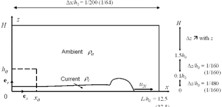
l/480 L... 0 (11160) e, 1 0 er _{Xo Uh} 0 = 12.5 (3ï.5)

Figure 1: Physical configuration used in the present work

and spatial resolution of the Navier-Stokes simulations. The dashed line represents the initial separation between fluids, while the solid line represents the interface at later times.

Here, the gravity vector is defined as

g=g(p. -pc)IIP. -Pelez, thus both bottom and top

density currents propagate on

z=O.

The spatial resolution is

identical for ail  except Â;:::18.75 for which the resolution is given in parenthesis.

Shallow-water model

In the following, we briefly describe the assomptions and equations used in the shallow-water model used in the

present work to obtain, among others, the height hN and the

velocity uN of the current's nose during the constant-speed

initial phase. We refer the reader to Ungarish (2007) for

more details about the model.

In the present model, we consider incompressible, immiscible fluids, and assume that the viscous effects are negligible (in both the interior and the boundaries). The thickness of the current is h(x,t) and its horizontal velocity

(z-averaged) is u(x,t). Initially, at t=O, h=ho and u=O. We

assume a shallow current which, formally, implies a

non-small, but not clearly specified, value of Â. To close the

system of equations an additional boundary condition is

specified at the front of the current located at xN. The model

makes use of the condition

(1)

where the Froude number, Fr, is a fonction of the depth

ratio

h!IH

and is taken to be the Benjamin's (1968) relation

given by

Fr(h IH) = (2- hNIH)(1- hNIH) .

[ ]

1/2

N (1+hNIH)

(2)

Further assuming that the instantaneous height of the current is constant along its body and that the energy in the

domain cannot increase, one can match the shallow-water

solution of the forward-propagating characteristic with Benjamin's front condition to obtain the height and velocity of the fronts. The height of the current is then given by the following implicit equation

where the Fraude number relation is given in (2). If we apply the additional energy consttaint, the maximum height of the current can be limited to H/2 and we obtain hN ""min(hN,H 1 2). The velocity of the current can then be determined from (1).

Navier-stokes solver

The numerical approach used here is the JADIM code developed at IMFT, Toulouse. Briefly, this code is a finite-volume method solviog the three-dimeosional, time-dependent Navier-Stokes equations for a variable-density incompressible flow (of arbitrary density variations), together with the density equation, assuming molecular diffusivity to be negligibly small. The transport equation of the density is solved using a modified Zalesak scheme (mixed low-orderlhigh-order scheme, Zalesak 1979). Momentum equations are solved on a staggered grid using second-arder centred differences for the spatial discretization and a third-order Runge-Kutta 1

Crank-Nicolson method for the temporal discretization. The incompressibility condition is satisfied using a variable-density projection technique. The overall algorithm is second-arder accurate in space and :first-order accurate intime. We refer the reader to Booometti et al.

(2008) and Haliez & Magnaudet (2009) for more details on the equations solved and the numerical technique.

In this approach, the transport equation of the density is hyperbolic. This is equivalent to choosing an infinite Schmidt number, defi.ned as the ratio of the kinematic viscosity to the molecular diffusivity. Although no physical diffusivity is introduced, the numerical thickness of the interface is not strictly zero as it is typically resolved over three grid cells (Bonometti & Magnaudet 2007). Therefore a finite effective Schmidt number can be estimated, which depends somewhat on the Reynolds number and

on

the degree of spatial resolution. Based on extensive tests of measurement of the interface thickness, Bonometti & Balachandar (2008) estimated that, for similar Reynolds number and spatial resolution as those used in the present work., the effective Schmidt number was of 0(103).

Thus, the numerical approach allows for the processes mixing and entrainment as one could observe in the transition region between weakly diffusive fluids (saltedlfresh waters for instance). Note however, that our simulations didn't detect any sigoificant entrainment in the range of density ratios investigated. We note in passing that we recorded the temporal evolution of the overall mechanical energy. In all the cases, the relative variation of the total energy remains negligibly small during the entire duratioo of the simulation (less than 0.1% ), indicating that the effect of numerical diffusion is marginal.

Numerlcal setup

The simulations reported here are two-dimensional and are performed within a rectangular (x,z) domain LxH large. In the following we set L=:12.5ho for a11 but the largest lock aspect ratio considered here; namely when Â=:l8.75 we choose L=:37.5ho (this configuration will be referred to as the long domain case as opposed to the short domain case,

and the characteristics of the long domain grid are given in parenthesis). We have paid careful attention to spatial resolution in order to en.sure grid-independent results. In particular, the grid is refined near the bottom boundary so as to accurately capture the front of the current, which is highly elongated in the high-density ratio configurations. We use a 2500x300 (2400x300) uniform grid with a spacing of Llx//Jo;;;;;;l/200 (1/64) in the x-direction. In the z-direction, the domain is divided into three regions. In the region 0 s;

z

s; O.lhu, a mùform spacing of .dz/ho==l/480 (1/160) is used, while a spacing of Liz/ho==l/160 (11160) is used over the region 01ho s;

z

s; l5ho (this region covers the density current and a significant portion of the ambient fluid entrained by the current). Finally, larger cells are used above

z=1.5ho,

following an arithmetic progression. Pree-slip boundary conditions for the velocity (unless otherwise specified) and zero normal gradient for the density are imposed on the top, bottom and lateral boundaries.

The computations to be described below were run at a prescribed Reynolds number Re"" Ubu 1 v of 2.5xHf, where U ""~ g'

ho

and g ';;;;;;gltJc-Pallmax(pc, pJ is the reduced gravity. We further assume the dynamical viscosity to be the sarne for both fluids (see e.g. appendix B of Bonometti et al. (2008) for a discussion of this assomption). Here we varied the density ratio in the range

1 O""" s; pc 1

pa

s; 104

• Note that in order to keep the Reynolds number constant while the density ratio varies, we modify the viscosity of the fluids accordingly.

Jas

j

6

1 t

x

0 +10 1

Figure 2: Temporal evolution of the shape of a top density current (shadowgraph) for lt=50 and pJpa=10-3. The time interval between successive views is lu~ g' 1

ho

= 2.827. Axes are scaled by

ho.

Large initiallock aspect ratios

In this section the initial lock ratio is fixed at the largest value  = 18.75. The shape of Boussinesq density currents of arbitrary initial depth ratios has been extensively described in the literature as weil as that of non-Boussinesq currents in the lock-exchange configuration. However, the description of non-Boussinesq top density currents in a deep ambient is much less documented. Therefore, we plot in figure 2 the temporal evolution of the shape of a top density

* 3

current (H =50 and pJpa=10- ). Soon after the removal of the gate, the head of the current is clearly visible and takes a rounded shape. At the same time, a surface perturbation is formed behind the head. The distance separating the surface perturbation from the current head is observed to grow in time while the height of the current remains approximately constant in between. Therefore, for the times considered here, the shape of the top density current can be decomposed into a head, a surface perturbation (note that sorne small vortical structures are discernable at the junction with the head) and a tail further downstream.

Since Â>> 1 here, it is reasonable to compare the speed of propagation obtained from the Navier-Stokes simulations with that predicted by the one-layer shallow-water theory in the constant-speed phase. The front velocity obtained from the Navier-Stokes simulations (symbols) is compared in figure 3 with the shallow-water model (tines), for density currents of various density ratios and two different initial depth ratios, namely H*=1 and 50, respective! y. Note that intermediate initial depth ratios were also investigated and the results were in essential agreement and therefore, for clarity, they are not presented here. The front velocity was computed as follows. For each simulation, we record the temporal evolution of the front position xN defmed as the maximum value of

x for which the equivalent

height

h

is non-zero, where

h

is defined as (Marino et al. 2005; Cantero et al. 2007)

(5)

Here p is the local value of the density field. The instantaneous speed of propagation uN is then computed as

UJFdxt/dt. For ali the Â=18.75 cases, an acceleration phase followed by a nearly constant phase (slumping) is observed. The agreement is fairly good in the case H*=1 (lock-exchange configuration) for the complete range of density ratio shown here. lndeed, the front velocity of top density currents ( 10-4 ~pc 1 pa ~ 1 ) predicted by the shallow-water model agrees within 1% with the simulations while for bottom density currents (1~Pc 1

Pa

~104_{) the}

maximum discrepancy is less than 10%. Such discrepancy was previously observed in Bonometti et al. (2008) for 10-1 _~Pc

_{1 Pa}

_~6x10-1_{, and was attributed to dissipation}

stemming from vortical structures generated near the front of the current.

For H* =50, good agreement is observed for bottom density currents ( 1 ~Pc

1

Pa~ 104

). In line with the shallow-water model prediction, the results become independent of H* as the density ratio increases. For instance, the front velocities of the H*=l and

ih

International Conference on Multiphase Flow ICMF 201 0, Tampa, FL USA, May 30-June 4, 2010 H*=50-currents are nearly identical for

Pc 1 Pa

=103

• The

situation is different for top density currents. As shown in figure 3, we observe an increasing departure between the predicted (solid line) and computed velocities as the density ratio is decreased. The shallow-water model overestimates the front velocity by at most 25% for the smallest density ratios investigated here. We also plot for comparison the experimental results of Rottman & Simpson (1983) in the B?ussinesq l!mit at intermediate initial depth ratios, namely H =4 and H ""15 (see the diamond and circle symbols). A monotonie increase in the velocity is observed from H* = 1 to H*=50. Comparison between the experimental results and the present computational results is in general quite good.

The fact that the largest error is observed for small density ratios could be expected. First, the shallow-water one-layer model becomes less and less accurate when H*

pJ

Pa

decreases because the inertia of the retum flow in the ambient (which is neglected in the shallow-water model) increases like (H*pJpar1• More precisely, Ungarish (2007) estimated that the effects of the ambient fluid on the dYllamics of the density currents can be neglected provided (H PdPar1<112 approxirnately. For H*=1 this leads to the condition pJpa>2. 1t can therefore be expected that the agreement between the simulations and the model breaks down for pJpa<2. However, an additional energy constraint arises for pJpa<l.373 (that is the flow is choked at half the initial depth). This sets the velocity of the current to be that imposed by the front condition, and as a result the agreement is excellent (see the comparison between the dashed line and the squares in figure 3). For H*=50, the condition for neglecting the ambient fluid dynamics reduces to pJpa>4x10-2• This is in reasonable agreement with our

results for which the discrepancy is maximum for density ratios in the range pJpa<4xl0-2 approximately. The fact that the speed discrepancy is at most 25% for a density ratio that is 400 times smaller than the limit of validity is actually an indication of the robustness of the shallow-water one-layer model. This robustness calls for sorne further theoretical and numerical investigation. Overall, we may conclude that one possible reason for the discrepancy between the shallow-water model and the computed velocities of top density currents in deep ambient is the fact that the model neglects the fluid motion in the ambient fluid. Thus, under such conditions a two-layer model, where both the motion of the current as weil as the ambient is taken into account can be expected to perform better. ' Second, there were indications that light currents are more dissipative than heavy currents (Birman et al. 2005; Bonometti et al. 2008). This trend, inferred from full-depth lock releases, was carefully investigated in the present systems. The Navier-Stokes results indicated that dissipative effects are larger for top currents than for Boussinesq or bottom currents. Indeed, for pJpa=10-2 (H*=10), the dissipation energy was found to be of 10% that of the kinetic energy; this is 4-5 times greater than for pj Pa= 1.01 and pj Pa= 102• This suggests that forlonger times, viscous effects may influence the propagation of the top current, inasmuch that the assumption of negligible viscous effects is not valid anymore.

o~~~~~~~~~~~~~~~~

10-4 _10-3 _10-2 _10-1 _{10° 10}1 ₁₀2 ₁₀3 ₁₀4

Pel Pa

Figure 3: Slumping front velocity as a function of the

density ratio. The solid (resp. dashed) line is the prediction of the shallow-water model for H*=50 (resp. H*=l). Triangles (resp. solid squares) are Navier-Stokes results for H*=50 (resp. H*=l). Crosses are numerical results of Birman et al. (2005) (H*=1). Experimental results of Lowe et al. (2005) (open square, H*=1) and Rottman & Simpson

(1983) (diamond, H*=4; circle, H*,15) are also plotted for comparison.

Third, it has been shown that the shallow-water prediction is quite sensitive to the choice of model for the front condition (2) in the case of high H* and small PdPa (Bonometti & Balachandar 2010). For instance for PdPa=10-2 , if one chooses the well-known empirical front condition proposed by Huppert & Simpson (1980) instead of (2), the value of front velocity predicted by the shallow-water model agrees within 2% (instead of 25%) with the Navier-Stokes results. lt should be stressed that it is therefore difficult to clearly disentangle the contribution of the fluid motion in the ambient (including inertia and dissipation) to that of the model for the front condition used in the shallow-water model on the observed discrepancy, so that no definite conclusion can be drawn at the present time. One alternative is to solve the more general shallow-water two-layer equations for arbitrary density ratios and initial depth ratios, so the inertia in the ambient fluid is included. The extension of the one-layer arbitrary density ratio shallow-water

model to two layers is not straightforward since it raises sorne non-trivial numerical issues. Overcoming these issues requires a substantial effort which is beyond the scope of the present work.

Arbitrary initial lock aspect ratios

The evolution of density currents is now considered for different values of the lock aspect ratio ~xofh0 ranging from 0.5 to 18.75. The density ratios investigated here range from top density currents to bottom density currents, while the initial depth ratio is set to H*=10. From the inspection of the temporal evolution of the front velocity, three regimes were observed (not shown here). (i) For large aspect ratio, greater than sorne critical value, say Àcrit• the propagation of the current was observed to be independent of the lock

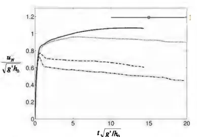
aspect ratio. For example, for PdPa~1, the ~18.75 and ~6.25 curves of utv(t) collapse. (ii) There exists an intermediate regime where the front velocity vs. time depends on the lock aspect ratio, but still a near constant velocity can be observed. (iii) For small aspect ratio, there is no constant velocity. This À-dependence is illustrated in figure 4, where the temporal evolution of the front speed is displayed for À ranging from 0.5 to 18.75 (p!pa=10-2). For comparison, we plotted as solid line the prediction of the shallow-water model (1)-(3) in the slumping regime. Clearly, the discrepancy between the Navier-Stokes results and the shallow-water prediction increases as À is decreased. These observations indicate that the speed of propagation of density currents is sensitive to the value of À. We may thus conclude that the front velocity is not only a function of Re, p!pa, and H* but of À. lt essentially decreases when À is decreased and the discrepancy is more significant for top density currents than for bottom density currents.

In the limit of light-top density currents, we derive a simple model showing that the front velocity uN scales like

À114• As mentioned above, the shape of the top density currents is characterized by a head of rounded shape followed by a nearly flat body. The angle made by the front of the current and the horizontal boundary is close to the value rt/3, as predicted by Benjamin (1968). Therefore, the volume tJ (per unit width) occupied by the fluid in the head of the current can be estimated as tf=

(41Z"-.J3)

h~

where

hN is the maximum height of the head. Here, we further assume that if the lock aspect ratio À is smaller than a critical value, say Àcr;r. then the fluid in the current is entirely located inside the head of equivalent volume and angle rt/3 (with respect to the horizontal boundary). Let V=xoh0 be the initial volume (per unit width) of the current.

We can write V

=

tJ which yields the following expression for the dimensionless height of the current

(6)

We argue that (1) is still a valid approximation for the speed of propagation, and bence, upon substitution of (6), we ob tain

(7)

The solution (7) is plotted in figure 5 (dash-dot line) and compared with the front speed obtained from the Navier-Stokes simulations (instantaneous values taken in a prescribed time interval). Also plotted is the slumping velocity predicted by the shallow-water theory (1)-(3). Predictions of (7) are in reasonable agreement with the computational results at small lock aspect ratios. As expected, as À increases the front velocity becomes independent of the lock aspect ratio and the speed of propagation is close to that predicted by the shallow-water theory. Note also that in the present configuration

(p/pa=10-2), the critical value of À for which the front velocity given in (7) is equal to that predicted by the shallow-water theory is À . _cru

""(47r-.J3)""

11.

1.2 ... ··-··· 0.8 UN f\''---

-J

g'

ho

0.6

\-

·-

·

--

·

-

·

-

·

--

·

-·

-

·-

-·-

·

-

·

--·~-~~

-~

:_~~-~~

·

-

·--

·-·-·--·-·-·-0.4 0.2 5 10

t~g'lho

15 20

Figure 4: Temporal evolution of the front velocity uN for

various lock aspect ratios  (p/p,.=10-2): - - , .Â-=18.75;

... , Â=6.25; ---, Â=1; -·-·-·-·-·-, Â=0.5. The

horizontal tines with circle represent the slumping velocity predicted by the shallow-water theory (eq. 1-3).

A.l/4

Figure S: Ranges of instantaneous front velocity (taken in a

time range Tj5.t5.TF) obtained from the Navier-Stokes

simulations vs. Â114 for top density currents (pJpa=l0-2;

d

=10). The solid vertical solid bars are uN in the time range

[T/T=2, TP'T=15]. For comparison we plotted as vertical

dotted bars uN in the time range [T /T=0.6, T P'T=15] which

includes the end of the acceleration phase. Observe that the trend is similar despite the amplitude of the variations is different.-, solution (7); ---, predicted slumping front

velocity from the shallow-water theory (1)-(3). Note that in

(7), we used Fr=1.27 as obtained from (2)-(3).

Summary

We carried out a numerical investigation of high-Reynolds number constant volume non-Boussinesq density currents propagating over a horizontal flat boundary in a deep

ambient. The goal is to shed light on the influence of the

density ratio and lock aspect ratio on the shape and

dynamics of the current. Solutions of the shallow-water

7111 International Conference on Multiphase Flow

ICMF 2010, Tampa, FL USA, May 30-June 4, 2010

equations were also used for comparison with the Navier-Stokes simulations.

In the accepted description, the high Reynolds number density current created by lock-re1ease, depends on:

(1) In the Boussinesq case, one free parameter, the initial

depth ratio H•; and (2) In the non-Boussinesq case, on two

parameters

If

and the density ratio, pJPa· Our results

highlight an additional parameter: ÂFXr)ho, which may play

a rote in bath Boussinesq and non-Boussinesq cases. It was

observed that the shape and speed of propagation of density

currents are influenced by the lock aspect ratio À, if  is

below a critical value

4nt-

The critical value of  depends

primarily on the density ratio p,!p,., and to a lesser extent, on

the initial depth ratio If. In the specifie case of light-top

density currents, we developed a simple model predicting

the dependence of the front velocity on Â. (for ÂI<Ât:r/t). The

speed of propagation

was

found to evolve as .Â-114, in

reasonable agreement with the Navier-Stokes results.

This work is just

a

preliminary report, and a more

sound and extended investigation will be presented in a

journal paper which is now in preparation.

Acknowledgment

MU thanks the University of Florida at Gainesville for

basting his academie visit during which a part of this research was carried ouL

References

Baines, W. D., Rottman, J. W. & Simpson, J. E. 1985 The

motion of constant-volume air cavities released in long

horizontal tubes. J. Fluid Mech. 161, 313-327.

Benjamin, T.B. 1968 Density currents and related

phenomena. J. Fluid Mech. 31, 209-248.

Birman, V., Martin, J. E. & Meiburg, E. 2005 The

non-Boussinesq lock-exchange problem. Part 2.

High-resolution simulations. J. Fluid Mech. 537, 125-144.

Bonometti., T., & Balachandar, S. 2008 Effect of Schmidt number on the structure and propagation of density currents.

Theor. Comput. Fluid Dyn. 22,341-361.

Bonometti., T., & Balachandar, S. 2010 Slumping of

non-Boussinesq density currents of varions initial fractional depths: a comparison between direct numerical simulations

and a recent shallow-water madel. Comput. Fluids 39,

729-734.

Bonometti., T., Balachandar, S. & Magnaudet, J. 2008 Wall

effects in non-Boussinesq density currents. J. Fluùi Mech.

616, 445-475.

Bonometti, T. & Magnaudet, J. 2007 An interface capturing

method

for incompressible two-phase :flows. Validation and

application to bubble dynamics. Int. J. Multiphas. Flow 33,

Cantero, M.I., Lee, J.R., Balachandar, S. & Garcia, M.H. 2007 On the front velocity of gravity currents. J. Fluid Mech. 586, 1-39.

Etienne, J., Hopfmger, E.J. & Saramito, P. 2005 Numerical simulations of high density ratio lock-exchange flows. Phys.

Fluids 17, 036601.

Gardner, G C. & Crow, 1. G. 1970 The motion of large bubbles in horizontal channels. J. Fluid Mech. 43, 247-255. Grobelbauer, H.P., Fannelfl)p, T.K. & Britter, R.E. 1993 The propagation of intrusion fronts of high density ratio. J. Fluid Mech. 250, 669-687.

Haliez, Y. & Magnaudet, J. 2009 A numerical investigation of horizontal viscous gravity currents. J. Fluid Mech. 630, 71-91.

Hartel, C., Meiburg, E. & Necker, F. 2000 Analysis and direct numerical simulation of the flow at a gravity-current head. Part 1. Flow topology and front speed for slip and no-slip boundaries. J. Fluid Mech. 418, 189-212.

Huppert, H. & Simpson, J. 1980 The slumping of gravity currents. J. Fluid Mech. 99,785-799.

Klemp, J. B., Rotunno, R. & Skamarock, W.C. 1994 On the dynamics of density currents in a channel. J. Fluid Mech.

269, 169-198.

Lauber, G & Rager, W.H. 1998 Experiments to dam-break wave: Horizontal channel. J. Hydraul. Res. 36,291-307. Lowe, R. J., Rottman, J. W. & Linden, P. F. 2005 The non-Boussinesq lock-exchange problem. Part 1. Theory and experiments. J. Fluid Mech. 537, 101-124.

Marino, B., Thomas, L. & Linden, P. 2005 The front condition for density currents. J. Fluid Mech. 536, 49-78. Martin, J.C. & Moyce, W.J. 1952 An experimental study of the collapse of liquid columns on a rigid horizontal plane.

Philos. T. Roy. Soc. A. 244, 312-324.

Ooi, S.K., Constantinescu, G. & Weber, L. Numerical simulations of lock-exchange compositional gravity currents. J. Fluid Mech. 635,361-388.

Ozgokmen, T., Fischer, P., Duan, J. & Iliescu, T. 2004 Three-dimensional turbulent bottom density currents from a high-order nonhydrostatic spectral element model. J. Phys. Oceanogr. 34,2006-2026.

Rottman, J. & Simpson, J. 1983 Density currents produced by instantaneous releases of a heavy fluid in a rectangular channel. J. Fluid Mech. 135,95-110.

Schoklitsch, A. 1917 Uber Dammbruchwellen. Sitzungsber.

Akad. Wissenchaft. Wien 26, 1489-1514.

Simpson, J .E. 1982 Gravity currents in the laboratory,

atmosphere and oceans. Annu. Rev. Fluid Mech 14, 213-234.

Spicer, TO. & Havens, JA. 1985 Modelling the phase 1 Thomey Island experiments. J. Hazard. Mater. 11,237-260. Stansby, P.K., Chegini, A. & Barnes, T.C.D. 1998 The initial stages of dam-break flow J. Fluid Mech. 374, 407-424.

Ungarish, M. 2007 A shallow-water model for high-Reynolds-number gravity currents for a wide range of density differences and fractional depths. J. Fluid Mech.

579, 373-382.

Ungarish, M. 2009 An introduction to gravity currents and

intrusions. Chapman & Hall/CRC Press.

Wilkinson, D. L. 1982 Motion of air cavities in long horizontal ducts. J. Fluid Mech. 118, 109-122.

Zalesak, S.T. 1979 Fully multidimensional flux-corrected transport algorithms for fluids. J. Comput. Phys. 31, 335-362.

Zukoski, E.E. 1966 Influence of viscosity, surface tension, and inclination angle on motion of long bubbles in closed tubes. J. Fluid Mech. 25, 821-840.