Characterization of solar X-ray response data from the REXIS instrument

Characterization of Solar X-ray Response Data from

the REXIS Instrument

by

Andrew T. Cummings

Submitted to the Department of Earth, Atmospheric, and Planetary

Sciences

in partial fulfillment of the requirements for the degree of

Bachelor of Science in Earth, Atmospheric, and Planetary Sciences

at the

MASSACHUSETTS INSTITUTE OF TECHNOLOGY

June 2020

c

○ Massachusetts Institute of Technology 2020. All rights reserved.

Author . . . .

Department of Earth, Atmospheric, and Planetary Sciences

May 18, 2020

Certified by . . . .

Richard P. Binzel

Professor of Planetary Sciences

Thesis Supervisor

Certified by . . . .

Rebecca A. Masterson

Principal Research Scientist

Thesis Supervisor

Accepted by . . . .

Richard P. Binzel

Undergraduate Officer, Department of Earth, Atmospheric, and

Planetary Sciences

Characterization of Solar X-ray Response Data from the

REXIS Instrument

by

Andrew T. Cummings

Submitted to the Department of Earth, Atmospheric, and Planetary Sciences on May 18, 2020, in partial fulfillment of the

requirements for the degree of

Bachelor of Science in Earth, Atmospheric, and Planetary Sciences

Abstract

The REgolith X-ray Imaging Spectrometer (REXIS) is a student-built instrument that was flown on NASA’s Origins, Spectral Interpretation, Resource Identification, Safety, Regolith Explorer (OSIRIS-REx) mission. During the primary science ob-servation phase, the REXIS Solar X-ray Monitor (SXM) experienced a lower than anticipated solar x-ray count rate. Solar x-ray count decreased most prominently in the low energy region of instrument detection, and made calibrating the REXIS main spectrometer difficult. This thesis documents a root cause investigation into the cause of the low x-ray count anomaly in the SXM. Vulnerable electronic components are identified, and recommendations for hardware improvements are made to better facilitate future low-cost, high-risk instrumentation.

Thesis Supervisor: Richard P. Binzel Title: Professor of Planetary Sciences Thesis Supervisor: Rebecca A. Masterson Title: Principal Research Scientist

Acknowledgments

I conducted my work as a research assistant with the REXIS program in the Space Systems Laboratory as a student in the MIT Department of Earth, Atmospheric, and Planetary Sciences and the MIT Department of Aeronautics and Astronautics. I owe this thesis to the dedication of countless friends, loved ones, faculty, and staff. Though there are too many to list, I wish to acknowledge a few:

First and foremost, I would like to express my gratitude to Dr. Rebecca Mas-terson for her guidance and encouragement in the past year. Thank you for always challenging me to grow and improve as an engineer, and for always believing in me.

I would like to thank my other advisor, Professor Richard Binzel, who first invited me to join the REXIS project, and whose passion for science motivated me to dream big and start down this road. Thank you for recognizing something in me, and for agreeing to advise just one last time. Additionally like to recognize the Harvard-Smithsonian Center for Astrophysics team of Dr. Branden Allen, Dr. Daniel Hoak, Dr. Jaesub Hong, and Professor Jonathan Grindlay for mentoring me. Many thanks to the REXIS cohort of Maddy Lambert, Carolyn Thayer, and David Guevel; I would do it all again for the laughs and camaraderie. Special thanks to Megan Jordan for tolerating endless paperwork and logistics, and at times, wrangling me in.

I would also like to thank my family for sending their love and support from so very far away. And to my friends: Lucy, Dan, Brandon, Ruth, Brendan, and Lara; Thank you for being the people who lifted me up when I was down, and for being with me all the way.

Lastly, I wish to thank the Halperin family, for welcoming me into their home during an unprecedented global crisis.

Contents

1 Introduction 13

1.1 REXIS Mission . . . 14

1.2 REXIS Operational Timeline . . . 16

1.3 Anomaly Resolution during the OSIRIS-REx mission . . . 17

1.4 Motivation . . . 18 1.5 Thesis Roadmap . . . 19 2 Background 21 2.1 Basic Circuitry . . . 22 2.1.1 Common Components . . . 22 2.1.2 Operational Amplifiers . . . 25 2.1.3 Signal Amplification . . . 27

2.1.4 Analog-to-Digital Signal Conversion . . . 29

2.1.5 Thermal Impact on Circuitry . . . 30

2.2 SXM Overview . . . 31

2.3 SXM Data Pipeline . . . 32

2.3.1 Instrument Response Modeling . . . 32

2.3.2 Chianti Atomic Database . . . 32

3 SXM Design and Operation 33 3.1 SXM Design Background . . . 34

3.1.1 Mission Requirements . . . 35

3.2 Instrument Testing . . . 42

3.2.1 Ground Testing . . . 42

3.3 Flight Operations . . . 45

3.3.1 Early Flight Operations . . . 45

3.3.2 Flight Operations during Orbital B . . . 46

3.3.3 Flight Operations during Orbital R . . . 47

4 SXM Root Cause Analysis 51 4.1 SXM Low Count Rate Anomaly . . . 52

4.1.1 Orbital B . . . 52

4.1.2 Orbital R . . . 54

4.2 Constraining the Problem . . . 54

4.2.1 ISA #10939 . . . 55

4.2.2 Modeling SXM Instrument Response . . . 60

4.3 LTSpice Simulations of Amplification Chain . . . 61

4.3.1 Thermal Variability in Components . . . 62

4.4 Root Cause Next Steps . . . 65

4.4.1 Identification of Vulnerable Components . . . 65

4.4.2 CAST Analysis . . . 65

A SXM Circuit Schematics 69 B Simulation Code 103 B.1 SXM Simulated Instrument Response Code . . . 103

B.2 SXM Histogram Rebinning . . . 107

List of Figures

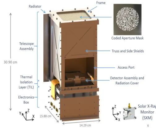
1-1 Schematic of the REXIS Instrument and SXM (shown to scale). . . . 15

2-1 The symbol used to represent a resistor in circuit diagrams. . . 22

2-2 The symbol used to represent a capacitor in circuit diagrams. . . 23

2-3 The symbol used to represent a diode in circuit diagrams. The positive terminal is to the left, and the negative terminal is on the right. . . . 24

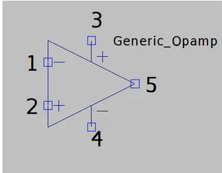
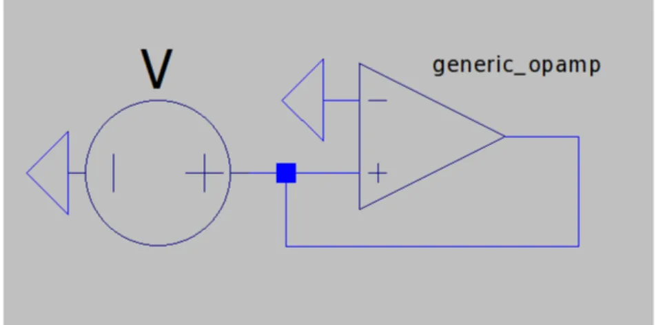
2-4 A generic op-amp. (1) Inverting input, (2) Non-inverting input, (3) Positive power supply, (4) Negative power supply, (5) Output. . . 25

2-5 A generic op-amp with open-loop gain. . . 26

2-6 A generic op-amp with closed-loop gain. . . 27

2-7 An example differentiator circuit. . . 28

2-8 An example integrator circuit. . . 28

2-9 An integrator circuit with an additional resistor added to the feedback loop provides a discharge path for the capacitor. . . 29

2-10 An example Schmitt Trigger. . . 30

3-1 The REXIS Requirements documentation flow from Jones, 2015 [6]. 35 3-2 SXM detector and preamp housing. The SXM detector is located below the collimator. . . 38

3-3 Schematic of SXM Amplification Chain. Outputs outb and outu are seen on the far right. . . 39

3-4 SXM Trigger Circuit Schematic. . . 40

3-6 SXM Histogram of Ground Calibration Source. A strong iron line can

be seen at around 200 ADU. . . 43

3-7 Results of SXM Oven Test, November 2015. . . 44

3-8 Temperature Fluctuations during the MEB Thermal Characterization Test. . . 44

3-9 Ground Testing results of MEB susceptibility to temperature fluctua-tions. . . 45

3-10 SXM Event Rate Histograms during L+30 . . . 47

3-11 SXM Event Rate Histogram from Orbital B, 25 July 2019. . . 48

3-12 SXM Event Rate Histogram from Orbital R, 13 November 2019. . . . 49

4-1 Example Fishbone diagram used to outline a Root Cause Analysis. Each bone is used to categorize the type of cause. . . 51

4-2 SXM count rate histogram from launch to Orbital R. . . 53

4-3 SXM Saturated Histogram (Right) and Corrected Histogram (Left) . 54 4-4 SXM count rate histogram on 18 November, 2019. The gap in the his-togram is when the instrument was not recording data, and is unrelated to the low count rate anomaly in Orbital R. . . 55

4-5 Fishbone diagram constructed for OSIRIS-REx ISA #10939 . . . 56

4-6 Flare Coincidence between the SXM and GOES15. . . 57

4-7 SXM longterm HV for its operational lifetime. . . 58

4-8 SXM Temperature Phase Space. . . 59

4-9 SXM Histogram Rebinning. The boxed area surrounds the SXM’s main signal peaks. The peaks at the outer edges of the figure are instrument artifacts. . . 61

List of Tables

3.1 Quantum Efficiency Requirements for the SXM Detector. . . 36

3.2 SXM Level 3 Requirements. . . 36

Chapter 1

Introduction

This thesis is intended to provide an overview of operations involving the REXIS Solar X-ray Monitor (SXM), and an investigation into the cause of unanticipated low solar signal seen during data collection. The SXM is a subunit of the REgolith X-ray Imaging Spectrometer (REXIS), which is mounted aboard NASA’s OSIRIS-REx mission.

REXIS an instrument intended to use to produce elemental abundance maps of the surface of the asteroid 101955 Bennu, a C-type near-Earth asteroid using spectrom-etry. Bennu is of particular interest because it has a 1-in-2700 chance of impacting Earth between 2175 and 2199 [9].

The SXM is a low-cost, high-risk payload. Isolating the root cause of the malfunc-tion and identifying critical components that resulted in failure will provide future projects with additional knowledge for instrument design. The SXM works in con-junction with the REXIS spectrometer to characterize high-energy solar x-ray flux. The SXM is used to detect variable input from the Sun, which is used by the REXIS spectrometer to calibrate x-ray input to Bennu. This thesis will provide an explana-tion of how solar x-rays are captured by the SXM and how signal data are interpreted. Solar spectra analysis and solar temperature fitting techniques are discussed, as well as the limitations of SXM modeling. SXM hardware is explained, with a focus on the analog signal amplification chain.

por-tion of the thesis will be on a root cause analysis of the low x-ray count-rate anomaly that occurred late in the SXM’s operational lifetime. This thesis will conclude with a roadmap for future work, including a more complete root cause investigation into thermal sensitivity, and a CAST analysis to highlight organizational and program-matic controls that may have contributed to the drop off in x-ray counts.

1.1

REXIS Mission

REXIS is a student experiment developed initially as part of the 2011 undergraduate capstone class in the Department of Aeronautics and Astronuatics at MIT. Construc-tion and management of the instrument was conducted in the MIT Space Systems Laboratory (SSL) as part of a larger collaboration with Harvard College Observatory (HCO), the MIT Department of Earth, Atmospheric, and Planetary Science, the MIT Kavli Institute (MKI), MIT Lincoln Laboratories, and Aurora Flight Sciences. Day-to-day operations and engineering are conducted primarily by students with guidance from senior faculty and staff including Professor Richard Binzel, the REXIS Instru-ment Scientist, Professor Jonathan Grindlay, the REXIS Deputy InstruInstru-ment scientist from HCO, and Dr. Rebecca Masterson, the REXIS Project Manager, from the MIT Department of Aeronautics and Astronautics. To date, over 80 students have worked on REXIS at all levels and stages of the project.

The REXIS main spectrometer relies on coded aperture mask spectroscopy to cap-ture incident x-rays from Bennu’s surface in the soft x-ray band (0.5-7.5 keV). A total x-ray spectrum is derived from the soft x-ray data and REXIS was designed to detect, if measurable, signals from Si, S, Mg, and O. REXIS has two operating modes: Imag-ing and Spectral. In imagImag-ing mode, REXIS maps specific abundances to locations on Bennu’s surface with necessary spatial resolution at an observation distance of 700m. In spectral mode, REXIS records x-ray energies and produces the global average of the x-ray spectrum passing through the coded aperture mask. REXIS performs its science objective in concert with the other OSIRIS-REx instruments.

of REXIS are housed in the main instrument. These consist of a 2x2 array of CCD’s housed within a coded aperture mask. Housed separately is the Solar X-Ray Monitor (SXM), which will be the focus of this study.

Figure 1-1: Schematic of the REXIS Instrument and SXM (shown to scale).

The SXM is an x-ray detector located on the outside of the spacecraft bus, so that it would be sun facing during observations of Bennu. The SXM is connected to REXIS by a coax cable, and SXM data processing occurs in the main REXIS instrument.

REXIS is the second student experiment to accompany a New Frontiers mission as part of NASA’s education and public outreach initiative. The first student instru-ment, the Venetia Burney Student Dust Counter (VBSDC, formerly SDC) built by University of Colorado Boulder, flew on the New Horizons spacecraft and recorded interplanetary dust from between 2.6 and 15.5 AU [13]. REXIS is a significant leap in complexity from the VBSDC, and at its inception was required to "directly engage students at the undergraduate and graduate levels in the conception, design, imple-mentation, and operation of space flight instrumentation. (2011 internal program

level doc.)"

1.2

REXIS Operational Timeline

This section will discuss the operational lifetime of REXIS and the SXM, from its launch on 8 September 2016 until the instrument’s planned shutdown following the OSIRIS-REx Orbital R mission phase in November 2019. A more detailed explanation of SXM operations can be found in Chapter 3. Henceforth, some operational times will be referred to as "L+", which stands for months after launch, unless otherwise specified. For example, events in the L+30 phase of the mission occurred 30 months after launch. The REXIS timeline is inherently linked to the OSIRIS-REx timeline.

REXIS was powered on during L+14 Days for a payload inspection and functions check. The SXM took 3935 seconds of x-ray data, and the instrument function was nominal. The SXM was turned on for an additional function check at L+6, where the instrument threshold was set. A third functions check was conducted during L+18. The SXM remained nominal, and there were no anomalies in x-ray detection.

The next big milestone was the L+22 Checkout in July 2018, where REXIS and the SXM were again checked for behavioral anomalies. Data collected by the SXM demonstrated full functionality. During L+22, REXIS was internally calibrated to identify background noise and hot pixels. As a diode detector, the SXM cannot have hot pixels in the same way as a charge-coupled device (CCD) detector.

REXIS performed its cover opening operation in September 2018. The radiation cover was released using a frangibolt, after which REXIS detectors were first exposed to the space environment. REXIS underwent a series of cosmic x-ray calibrations (CXB), and the REXIS spectrometer was shown to be sensitive to stray light.

The L+30 Calibration was the first time Bennu was observable in the REXIS field of view. During this calibration, a hot pixel mask was tested on REXIS. SXM count rates were lower than previous observations, but returned to previously seen levels in later flight.

Scorpius X-1 (Sco-X-1), two known cosmic ray sources. Using a known, stable x-ray emitter provided a source that allowed the gain and offset of the REXIS detector nodes to be set. Crab Calibration took place in November 2018 and March 2019, while Sco X-1 occurred later, during Mask Calibration.

Orbital B, the first REXIS observation phase, occurred from 1 July to 6 August, 2019. This was initially the only observation window for REXIS. The OSIRIS-REx spacecraft was placed in a stable orbit one kilometer above the surface of Bennu. The SXM count rate saturation anomaly was found during Orbital B, where the instrument reported abnormally high counts on the detector. On 5 July, SXM data was saturated with an additional value of 34880. It was believed that a "bit flip" occurred, where radiation moved the reset value on the SXM. This was corrected with a reset command from the ground.

Additionally, throughout Orbital B the SXM began showing a two order of mag-nitude decrease in x-ray signal disproportional to the spacecraft’s solar distance. The results from results from the SXM’s Internal Calibration are depicted in Figure 4-2. More on this anomaly can be found in Chapter 4. In all, two anomalies were detected in the SXM, and three were detected in REXIS. For more information on REXIS anomalies, consult Maddy Lambert’s thesis [7].

Orbital R was the final observation window for REXIS, which occurred during November 2019. The REXIS team petitioned for, and was awarded, this additional observation to supplement limited data taken during Orbital B.

1.3

Anomaly Resolution during the OSIRIS-REx

mis-sion

Anomaly detection for instruments on OSIRIS-REx was primarily the job of the engineers and scientists behind the individual instrument. Generally, a few weeks were allotted after reporting the anomaly to conduct an investigation, and isolate the root cause.

After an assessment had been made, the instrument team would present a rec-ommendation for how to proceed with using the instrument to the OSIRIS-REx PI. This recommendation included an identification of the incident, current results of the investigation, and conclusions about future instrument performance and how it might affect the spacecraft. The investigation could be closed without reaching a defined root cause, so long as the incident was isolated and did not impact other instruments on the spacecraft.

1.4

Motivation

Low-cost, high-risk spaceflight missions granting better accessibility to space than ever before. The REXIS project was developed with the philosophy of being a student instrument. From its inception as the final deliverable for 16.83, the MIT Aerospace Engineering senior design capstone class, where undergraduate students worked side-by-side with experienced research scientists and engineers. Students directly applied s learned in their undergraduate curricula, and produced an instrument of complexity, scale, and mission worthy of being included on a New Frontiers spacecraft. Like all projects, there were challenges faced along the way. A rotating ensemble of students created a challenging environment for informational and experiential entropy.

The REXIS instrument is categorized as a NASA Risk Class D mission, which is characterized by lower cost and the use of legacy hardware [11]. Indeed, a portion of the electronics design process for REXIS consisted of utilizing existing schematics from NICER, an x-ray instrument developed by the MIT Kavli Institute (MKI). These schematics were simplified for the design of the SXM as a matter of reducing cost. Identifying the source of the SXM spaceflight anomaly not only provides guidance on potential hardware vulnerabilities which exist in current spaceflight missions; it also yields a roadmap for future missions.

1.5

Thesis Roadmap

This thesis is organized into six chapters, which document the SXM background, instrument anomaly, and subsequent investigation. The current chapter has intro-duced the larger REXIS mission, operations over its lifetime, and how anomalies were identified, catalogued, and solved. Chapter 2 presents a background on the SXM, including an explanation of the SXM data pipeline and associated solar x-ray modeling. A broad overview of the electronic components that comprise the SXM will be provided, as well as how they operate in the space environment. In Chapter 3, the structure and design process of the SXM will be explained in greater detail. This is followed by a summary of instrument testing that occurred, both on the ground and after launch. Then, SXM flight operations leading up to and after the anomaly are discussed. Chapter 4 explores the SXM root cause analysis. The identification of the low count-rate anomaly is explained in depth. The investigation into the SXM pre-amplification chain electronics is next. The chapter ends with a plan for future research into the identification of the vulnerability that caused the anomaly and how such a finding may be interpreted.

Chapter 2

Background

This chapter will describe the circuitry used in the SXM. The SXM relies on an intricate array of amplifiers and filters, which are capable of x-ray detection when combined. The chapter will begin with an introduction of standard electrical com-ponents and how they operate. An example circuit of each component is provided and includes a visual representation of ideal operation. This will create a foundation of understanding that will translate to more complex electrical engineering systems seen in the SXM. The first advanced concept explained is signal amplification. Signal amplification is the primary means through which a signal is passed from the SXM detector and recorded by the instrument. Typical amplification techniques will be compared against amplification used in the SXM. To understand signal processing in the SXM, an explanation of analog-to-digital conversion is provided. A more thor-ough model of SXM signal processing is covered later in the chapter. The thermal sensitivity of electrical systems is explained, and typical response sensitivities are modeled. An overview of the SXM will explain the functions of the instrument in broad terms. The SXM Data Pipeline will be explained from end-to-end. A theoret-ical solar x-ray response will be followed from detection, through the pipeline, and finally to transmission to the ground. Finally, the chapter concludes with theoretical instrument response using the Chianti Atomic Database and an explanation of how it was implemented in the Data Pipeline. SXM instrument simulation code can be found in Appendix B.

2.1

Basic Circuitry

This section introduces the common electrical components used in the SXM, how they operate individually, and how they are used together to create more complex circuitry.

2.1.1

Common Components

Resistor

Figure 2-1: The symbol used to represent a resistor in circuit diagrams.

A resistor is an electrical element with a positive and negative terminal that utilizes the property of electrical resistance. Its primary functions include voltage division, current flow reduction, and signal reduction. Ideal resistors function based on Ohm’s law,

𝑉 = 𝐼𝑅 (2.1)

where the voltage differential across the resistor is proportional to the product of current and resistivity. Resistors are commonly used in two constructions: parallel and series. Resistors in parallel are be treated as the multiplicative inverse of the sum of the reciprocals of individual resistors,

1 𝑅𝑒𝑞 = 1 𝑅1 + 1 𝑅2 + . . . + 1 𝑅𝑛 . (2.2)

Series resistors are treated as the sum of individual resistances,

𝑅𝑒𝑞 = 𝑅1+ 𝑅2+ . . . + 𝑅𝑛. (2.3)

.

capacitance in alternating current (AC) systems. These vulnerabilities are expressed primarily in the high frequency regime, which can impact signal amplification. Re-sistors are thermally emissive as a property of power dissipation. Power dissipation in an ideal resistor is modeled as

𝑃 = 𝑉

2

𝑅 = 𝐼

2_{𝑅 = 𝐼𝑉. (2.4)}

This power is converted to heat and emitted by the component.

Capacitor

Figure 2-2: The symbol used to represent a capacitor in circuit diagrams.

A capacitor is a passive, two terminal component that stores electrical charge. When a voltage potential is passed along a capacitor, an electrical charge is produced. A capacitor consists of two charged conducting nodes separated by a non-conductive medium. This medium consists of either a vacuum or a dielectric material, which can increase the capacitance of the component. Capacitors are characterized by their capacitance. In an ideal capacitor, its capacitance is measured as the ratio of charge held to the voltage across the component. This is represented in the formula

𝐶 = 𝑄

𝑉 (2.5)

in a DC system. In AC systems, a capacitor’s impedance influences the capacitance of the system. Impedance can be considered as a vector quantity described as the sum of the resistance and reactance, which is the component’s opposition to current. Impedance is inversely related to capacitance and signal frequency.

The characteristics of capacitors in parallel and series are exactly opposite of a resistor. The capacitance of multiple capacitors in parallel are be calculated as the

sum of the capacitance of the individual components. This is represented by the equation

𝐶𝑒𝑞= 𝐶1+ 𝐶2+ . . . + 𝐶𝑛. (2.6)

For capacitors in series, the total capacitance can be calculated as the multiplicative inverse of the sum of the reciprocals of individual resistors and represented by the formula 1 𝐶𝑒𝑞 = 1 𝐶1 + 1 𝐶2 + . . . + 1 𝐶𝑛 . (2.7) Diode

Figure 2-3: The symbol used to represent a diode in circuit diagrams. The positive terminal is to the left, and the negative terminal is on the right.

A diode is a unidirectional conductor that passes current from a positive to neg-ative terminal, and restricts current flow in the reverse direction. A typical diode utilizes a p-n junction material to generate a forward direction with zero resistance, and a backward direction of infinite resistance. A diode has two response modes known as reverse-bias and forward-bias. A diode that is reverse-biased will act as an insulator and will ideally prohibit current from being passed, so long as its volt-age limit is not exceeded. Conversely, a diode that is operating with a forward-bias will become a conductor, and current can pass backwards through the diode. Diodes also possess a property known as breakdown voltage, which flips a diode’s bias when reached. When a diode is exposed to its breakdown voltage in the direction opposite the flow of current, the formerly infinite resistance drops to low resistance, and cur-rent backflows. This property is exploited to direct curcur-rent in anomalous situations such as overvoltage. When an overvoltage situation occurs, a diode will switch from being negative-biased to being positively-biased, and will direct current away from sensitive components. Additionally, diodes have a characteristic voltage drop in the

direction of current flow, which is described in its commercial datasheet. This can be used to help shape a voltage in signal processing.

Gain

In analog amplification systems like the SXM, gain refers to the ratio of output to input signal. Voltage gain will be primarily discussed henceforth, as this is what occurs in the SXM amplification chain, although power, amplitude, and current are all other methods of measuring gain.

2.1.2

Operational Amplifiers

An Operational Amplifier, or op-amp is a high-gain voltage amplifier that takes a differential input and produces a single output. It is directly coupled, meaning that it relies on direct current transmission, rather than through inductive or capacitive coupling [2]. In a circuit diagram, an op-amp has five terminals, which are labeled in Figure 2-4.

Figure 2-4: A generic op-amp. (1) Inverting input, (2) Non-inverting input, (3)

Positive power supply, (4) Negative power supply, (5) Output.

Additionally, an ideal op-amp has the following characteristics [2]: ∙ No output impedance

∙ No DC offset in the output signal ∙ Infinite bandwidth

∙ Infinite input impedance ∙ Infinite open-loop voltage gain

Open-loop gain is entirely dependent on the input. Consider Figure 2-5 in which an op-amp is placed in the open-loop configuration. For any non-zero voltage input, the open-loop gain drives the op-amp output into saturation. When the op-amp is saturated, the output voltage no longer increases. When the voltage input to the op-amp is zero, the output from the op-amp is also zero. An op-amp in the open-loop configuration is liable to latch-up, where the op-amp experiences a short circuit and ceases to work. Op-amp saturation is not always reversible, and can permanently disrupt current flow through the circuit.

Figure 2-5: A generic op-amp with open-loop gain.

In order to guard against voltage output saturation, an op-amp can be configured for closed-loop gain, as shown in Figure 2-6. Closed-loop gain relies on the output signal feeding back into the input in order to shape desired input. Op-amps that amplify through the use of closed-loop gain are less susceptible to voltage saturation through amplification. However, it should be noted that saturation can still occur through overvoltage from the input.

Figure 2-6: A generic op-amp with closed-loop gain.

2.1.3

Signal Amplification

The SXM uses a signal amplification chain to shape and condition x-ray flux signal for analog-to-digital conversion. Two different input configurations will be discussed in this section, and select common amplification circuits will be explained.

Inverting amplifiers take a positive DC voltage at the input and produce a larger

negative voltage at the output. In AC amplification, the output is exactly 180 ∘)

out of phase with the input. Non-inverting amplifiers take an AC input and preserve its phase in the amplified output. A positive voltage DC input will yield a positive voltage output.

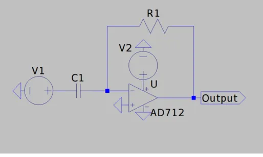
The first common amplification circuit is a differentiator, shown in Figure 2-7. A differentiator is created using an inverting amplifier with a capacitor in the input line, and a resistor in the negative feedback loop, which can be considered a rudimentary high-pass filter. This causes the output from the op-amp to be proportional to the time derivative of the input, which is where the circuit owes its name. The differentia-tor has a few characteristic limitations. For instance, a differentiadifferentia-tor is susceptible to circuit noise which may be amplified in the output. A differentiator is also susceptible to high-frequency noise, which can cause instability [2].

Similar to the differentiator, an integrator is used to integrate and invert an input signal. The output voltage is the time-dependent integral of the input voltage [2]. In

Figure 2-7: An example differentiator circuit.

this configuration, a resistor is included on the input line, and a capacitor is placed in the negative feedback loop, which creates a low-pass filter, as shown in Figure 2-8.

Figure 2-8: An example integrator circuit.

In its simplest configuration, an integrator circuit requires periodic discharge of the capacitor, which can become saturated with charge. When this occurs, the output voltage can drift beyond the optimal range of the op-amp. One way to mitigate this

challenge is to include a resistor in the feedback loop that functions as a discharge path for the loop capacitor (Figure 2-9).

Figure 2-9: An integrator circuit with an additional resistor added to the feedback loop provides a discharge path for the capacitor.

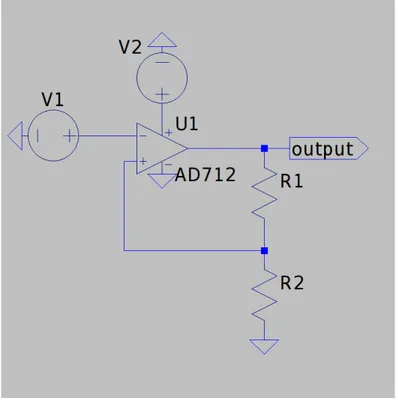
The last configuration worth mentioning is the Schmitt Trigger, which shapes an input signal into a square wave. An example Schmitt Trigger is provided in Figure 2-10. This configuration can be used to shape a signal at a set voltage, so that it can achieve a more lossless input into an analog-to-digital converter. A Schmitt Trigger is a modified integrator with positive feedback. A voltage divider is used to set the positive feedback, and looped back to the non-inverting input. When a prescribed threshold voltage is exceeded, the input voltage triggers and changes the state of the output voltage. This configuration is vulnerable to hysteresis effects, where the input voltage is above the threshold voltage.

2.1.4

Analog-to-Digital Signal Conversion

Analog-to-digital conversion is the process through which an analog signal is trans-lated into a series of digital values using an analog-to-digital converter (ADC). In the SXM, an input x-ray signal is amplified and shaped before being converted and digitized for data processing. The digital output from the ADC is proportional to the

Figure 2-10: An example Schmitt Trigger.

analog input signal, and is limited by quantization speed and accuracy concerns.

2.1.5

Thermal Impact on Circuitry

Temperature concerns must be accounted for when creating and operating complex electrical systems. Amplification circuits often have a small window of acceptable in-put voltages, and signals must remain within specified bounds in order to be amplified and ultimately converted by an ADC. Furthermore, unwanted over- or under-voltage can cause temporary or even irreversible damage to sensitive electrical systems.

While voltage itself is not thermally dependent, individual circuit elements are dependent. For instance, an increase in temperature can affect power dissipation in resistors. This can cause permanent damage to resistors by burning or melting the resistor. In capacitors, temperature can alter how charge moves within a dielec-tric material, increasing or decreasing the amount of charge required to saturate the component. Additionally, resistivity in the wiring connecting circuit elements scales positively with temperature, which can cause unintended voltages within the circuit.

Temperature concerns are considered in the design process of space hardware. For Class D missions, NASA recommends that only Level 1, Qualified Manufacturer List Class V (QMLV) legacy hardware is used in instrumentation. Circuitry tested to this level is rated for interplanetary spaceflight, where extreme radiation and thermal conditions are experienced [10].

2.2

SXM Overview

The SXM component of the REXIS instrument suite is a subassembly located on the OSIRIS-REx bus such that it will face the sun during windows of operation that REXIS is pointed at Bennu. The electrical elements of the SXM are attached to the REXIS Main Electronics Board (MEB) by a coax tether. The SXM mechanically adheres to the spacecraft bus using an aluminum mounting bracket. The external elements of the SXM consist of an Amptek XR-100SSD silicon drift diode (SSD) de-tector connected to a pre-amplification circuit (henceforth referred to as the preamp) located on a mounted printed circuit board (PCB).

When a solar x-ray hits the SSD detector, an analog signal is passed through the preamp, where it is conditioned and sent to the MEB. At the MEB, the analog signal passes through an ADC, which outputs a digital response. This digital response is processed further by the MEB into x-ray energy event histograms sorted by energy level. Event energy data is kept in Analog-to-Digital Units, which can be converted to units of Electronvolt (eV). A conversion from ADU to eV is calculated using the formula

𝑘𝑒𝑉 = 0.0219 * 𝐴𝐷𝑈, (2.8)

for the REXIS SXM.

Solar x-rays and their energies are then used to calculate the influx and energy of primary solar x-rays onto Bennu. A knowledge of primary x-ray energies is required to calibrate the secondary x-ray fluorescence capture by the REXIS detector.

2.3

SXM Data Pipeline

The SXM Data Pipeline takes a converted signal from the SXM ADC and processes it into data packets that are transmitted to the ground.

2.3.1

Instrument Response Modeling

The SXM underwent a series of ground and in-flight validations between 2013 and 2019. This section will focus on the instrument response modeling that was used to verify early in-flight observations. The SXM Data Pipeline included a model of ideal SXM response, which at its core took a sample time-series of x-ray detections and produced energy histograms. These energy histograms could then be fitted to a known solar abundance model, which would match an input signal to x-ray characteristics of elements in the Sun’s photosphere, and subsequently constrain solar temperature at the time of x-ray emission. While this function fell beyond the original scope of the SXM’s purpose, it provided yet another way to produce instrument science.

2.3.2

Chianti Atomic Database

The Chianti Atomic Database was used to create an instrument response model across all temperatures and energies observable by the SXM. The Chianti Database is an atomic spectra database built and maintained by a global consortium of atomic sci-entists [8]. Chianti and its associated python package, ChiantiPy, allow a user to generate model spectra of astrophysical bodies. For the purposes of the SXM, Chi-anti provided a known database against which sample SXM histograms could be matched. Both coronal and photospheric abundance models were generated at the temperatures and energies observable by the SXM, and ideal instrument response was cross-referenced against early in-flight calibration data that was taken prior to the REXIS instrument’s primary observation window. The intention of this cross-reference was to build reasonable confidence in the instrument response model such that temperatures and spectra abundances could be derived from data collected dur-ing observation.

Chapter 3

SXM Design and Operation

This chapter describes the design process and flight operations of the REXIS Solar X-ray Monitor (SXM). The first section will focus on the design constraints of the instrument. REXIS is a Risk Class D mission, which means it is a low budget instru-ment, and is designed to use legacy, off-the-shelf components [11],[12]. This section also describes the science mission requirements for the SXM, as well as design re-quirements stipulated by the OSIRIS-REx team. The design section will primarily detail the development of the SXM signal amplification chain, which is at the center of the Root Cause investigation found in Chapter 4.

The next section of this chapter will describe the testing battery used to char-acterize the SXM on the ground and in flight. The SXM’s pre-flight ground testing regimen will include testing data relevant to the SXM root cause analysis, and in-clude rationale for why some tests were foregone. Results of SXM flight testing will be presented, and nominal x-ray count data will be shown.

The last section of this chapter summarizes SXM flight operations. A timeline of operations is included to understand where flight testing occurred relative to science observations. Flight operations are separated into three distinct phases, which corre-late to OSIRIS-REx mission phases. Early flight operations are described, followed by operations during Orbital B and Orbital R, the SXM’s two science operation phases.

3.1

SXM Design Background

The SXM was first designed as part of the 16.83 undergraduate capstone class in the MIT Department of Aeronautics and Astronautics in 2011. This first design became the foundation upon which the SXM flight model was developed. The REXIS instrument was designed to use heritage spaceflight technology to reduce the design timeline. The SXM detector is an Amptek XR-100SDD, which is an updated model of detectors flown on previous x-ray instruments. The XR-100SDD is an updated version of the XR-100CR, and the former uses a silicon drift diode, while the latter uses a PIN photodiode [1]. Both models a beryllium window above an evacuated chamber in which the detector is housed. Amptek XR-100CR detectors were used in the Solar X-ray Spectrometer aboard GSAT-2, a space-based Indian solar observatory [5]. A similar Russian space observatory used the XR-100CR in the Solar Photometer in X-rays (SphinX) instrument [15]. Both of these previous instruments demonstrated that the Amptek XR-100 class detector could be reasonably be used to for x-ray solar observation, despite the XR-100SDD never having flown prior to REXIS.

The XR-100SDD detector was also included in early designs of the Neutron star Interior Composition ExploreR (NICER) instrument. NICER was developed by the MIT Kavli Institute (MKI), and the engineering teams worked closely together in the development processes. Both Professor Richard Binzel and Dr. Rebecca Masterson, who represent two-thirds of REXIS leadership, are affiliated with the Kavli Institute. Additionally, the Kavli Institute is located in the same building as the REXIS team,

meaning collaboration was as easy as going upstairs. Additionally, the Goddard

Spaceflight Center serves as the managing center for both REXIS and NICER. This closeness of personnel was reflected in the design of the REXIS SXM.

The NICER instrument is mounted aboard the International Space Station, where its main spectrometer observes neutron stars in the 0.2 to 12 keV range [4]. The REXIS SXM shares both structural and electronic heritage with the NICER instru-ment. An early design of NICER implemented 56 XR-100SDD detectors, the same detector used by the REXIS SXM. The NICER team later changed their design to

use an Amptek CMOS detector, which benefits from higher temporal resolution. While the NICER instrument and the REXIS SXM’s designs diverged during the design phase, the SXM was heavily influenced by this early NICER design. The design of the SXM preamp circuit and SXM Electronics Board resemble the NICER pream-plifier board and surrounding electronics housing respectively. These similarities are the legacy of John Doty, an engineer affiliated with MIT who created the SXM timing circuitry, signal pulse shaping, and threshold trigger. A complete documentation of SXM circuit diagrams can be found in Appendix A.

3.1.1

Mission Requirements

REXIS SXM requirements fall under the REXIS instrument’s main requirements, which in turn are derived from OSIRIS-REx requirements for the instrument. The REXIS requirements documentation flow was described extensively in Mike Jones’s Master’s thesis [6]. The information flow diagram for REXIS is shown in Figure 3-1

Figure 3-1: The REXIS Requirements documentation flow from Jones, 2015 [6]. The SXM’s energy band of interest is from 0.6 keV to 6 keV. Quantum efficiency for the SXM is also outlined in the REX-74 requirement. Quantum efficiency is the

ratio of photon events that are successfully converted to electrons by the detector, and is a metric used to evaluate the performance of an instrument at different detection energies (shown in Table 3.1).

Quantum Efficiency Energy Range (keV)

>0.01 0.62 - 0.7 >0.03 0.7 - 0.8 >0.09 0.8 - 1.2 >0.65 1.6 - 2.8 >0.85 2.8 - 4.1 >0.9 6.0 - 7.0

Table 3.1: Quantum Efficiency Requirements for the SXM Detector.

The REXIS SXM Requirements are derived from the different levels of REXIS requirements. SXM operational and environmental requirements are found in the Level 4 documentation. Level 3 documentation describes the requirements for detec-tor functionality. The Level 2 requirement REX-7 is the highest-level requirement pertaining to the SXM. REX-7 requires that the SXM "shall measure solar coronal temperature to within 0.1 MK every 50 sec while observing Bennu in Phase 5B as-suming a single temperature model." A complete overview of Level 3 and Level 4 requirements can be seen in Tables 3.2 and 3.3.

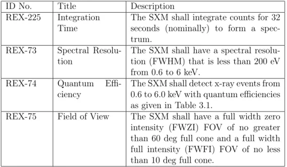
ID No. Title Description

REX-225 Integration

Time

The SXM shall integrate counts for 32 seconds (nominally) to form a spec-trum.

REX-73 Spectral

Resolu-tion

The SXM shall have a spectral resolu-tion (FWHM) that is less than 200 eV from 0.6 to 6 keV.

REX-74 Quantum

Effi-ciency

The SXM shall detect x-ray events from 0.6 to 6.0 keV with quantum efficiencies as given in Table 3.1.

REX-75 Field of View The SXM shall have a full width zero

intensity (FWZI) FOV of no greater than 60 deg full cone and a full width full intensity (FWFI) FOV of no less than 10 deg full cone.

ID No. Title Description

REX-228 SDD Survival

Temperature

The temperature of the SDD shall

al-ways be greater than -65∘C and less

than 150∘C.

REX-229 SDD Operating

Temperature

The temperature of the SDD shall be

less than -30∘Cand greater than -70∘C.

REX-76 Preamp Survival

Temperature

The temperature of the SXM Preamp

shall be greater than -55∘C and less

than 85∘C.

REX-77 Preamp

Operat-ing Temperature

The temperature of the SXM preamp

shall be greater than -40∘C and less

than 85∘C while operating.

REX-78 SXM Health The SXM shall survive and remain

op-erational through the end of Phase 8.

REX-79 SXM

Opera-tional Time

The SXM shall be capable of operating 24 hours per day

Table 3.3: SXM Level 4 Requirements.

3.1.2

Overview of SXM Signal Amplification Chain

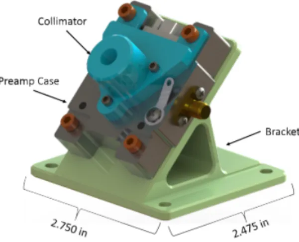
The SXM amplification chain is responsible for priming a signal from the SDD de-tector before it is converted by the Analog-to-Digital Converter (ADC). The amplifi-cation chain is housed on the SXM Main Electronics Board (MEB), which is located within the REXIS instrument on the spacecraft. The SXM detector and preamp cir-cuit are housed in the SXM backpack, which is bolted to the outside of the spacecraft, and is connected to the MEB by a coaxial cable. The SXM detector housing is shown in Figure 3-2.

The SXM ADC requires a positive voltage signal pulse to be passed to it in order to register a detection count. When an x-ray strikes the detector, an analog signal pulse is created. The raw signal biased at 3.3 V, sent through the preamp, and then sent across the coax cable to the MEB. When the signal reaches the MEB, it is passed through three opamps, which amplify the signal. Then the voltage signal is divided, where one signal passes through an integrator circuit and the other signal through a differentiator circuit. The output from the integrator circuit is labeled outu, and the output from the differentiator circuit is labeled outb. The amplification chain schematic diagram is shown in Figure 3-3. Additional SXM electronics schematics

Figure 3-2: SXM detector and preamp housing. The SXM detector is located below the collimator.

can be found in Appendix A.

The signals are then sent through a low pass filter to eliminate high frequency noise artifacts added to the signal when it passed through the preamp circuit. The outu signal is then sent to the final section of the amplification circuit, where 3 V of bias are subtracted, leaving the signal with a residual 0.3 V bias. This bias is required to keep the outu signal positive because the ADC used in the SXM electronics chain is not rated for negative voltage inputs.

Next, Signal outu is sent to the ADC to be measured, while signal outb is sent to a zero cross monitor, which provides the timing for the ADC to sample new signal, now named outu1.

In order to trigger an ADC detection, the SXM relies on a trigger circuit that uses a series of comparators to compare outb to a reference voltage. The trigger circuit is shown in Figure 3-4.

This trigger includes a command to manually set the threshold Voltage Lower Limit of Detection (VLLD). The VLLD is set above the outb bias voltage as well as the noise floor to prevent the SXM from accidentally triggering due to random noise in the electronics. The relationship of outb to VLLD is given as:

Figure 3-3: Sc hema tic of SXM Amp lification Chain. Outputs outb and outu are seen on the far righ t.

Figure 3-4: SXM Trigger Circuit Schematic.

where LLD is the Lower Limit of Detection. A threshold setting anomaly was discov-ered early in flight, where the threshold would fluctuate. This was resolved by sending

three threshold setting commands to the instrument. The first two commands were to set the threshold to an arbitrarily high value, and the third command was to set the threshold to the intended value. This workaround was only used once, but resolved noticeable threshold drift for the remainder of flight.

The second threshold circuit is used to determine the zero crossing of outb. When outu1 is at it’s peak, outb will have a zero crossing, and the ADC is triggered to begin recording. Figure 3-5 shows an example of all signal shapes.

3.2

Instrument Testing

As part of the instrument design process, the REXIS SXM was subject to numer-ous functionality tests on the ground. Testing was limited by time and financial constraints, but the testing framework was rigorous and proved the SXM ready for flight. The subsection on ground testing will focus on testing that aided in charac-terizing the SXM low count rate anomaly discussed in Chapter 4. A more thorough description of SXM ground testing can be found in Kevin Stout’s thesis [14].

The SXM also underwent a series of flight tests between launch in 2016 and Orbital B, the first data collection phase, in July of 2019. Flight testing was primarily used to characterize the REXIS main spectrometer, whose CCD array required in-flight calibration, although the SXM was tested as well [7].

3.2.1

Ground Testing

The SXM was put through a battery of ground tests to ensure the instrument was ready for flight testing. The testing procedure followed NASA requirements for Risk Class D missions [11]. The focus of this subsection will be on SXM thermal tests, which provided a background for the root cause analysis outlined in Chapter 4.

The SXM was subject to thermal testing using thermal vacuum chambers built in the MIT Space Systems Laboratory and at MIT Lincoln Laboratory.

SXM Oven Test

The SXM MEB underwent an oven test at Lincoln Laboratory in November of 2015. The complete SXM flight assembly, including the preamp and SDD detector, were placed in a thermal chamber. The MEB remained connected to the SXM assembly, but outside the chamber. The MEB was held at a temperature of approximately

20∘C. The temperature of the thermal chamber was then fluctuated between -40∘C

and 60∘C with a ground calibration iron source to measure instrument performance

as a function of temperature. This was a more drastic temperature fluctuation than was expected in flight, and was used to identify thermal vulnerabilities in the SXM.

An example histogram from the ground calibration source is shown in Figure 3-6.

Figure 3-6: SXM Histogram of Ground Calibration Source. A strong iron line can be seen at around 200 ADU.

The preamp and SDD detector remained insensitive to temperature fluctuations over the test range. Additionally, it was discovered that both low and high energy

artifacts set in at approximately 53∘C. The results of this test are provided in Figure

3-7.

MEB Thermal Characterization

The SXM MEB was included in a similar thermal test. The MEB was placed in

the thermal test chamber, where its temperature was then cycled between -40∘C and

60∘C, while the SXM was exposed to the Fe-55 ground calibration source. Figure 3-8

shows temperature changes in the SXM during testing.

At high temperatures, the SXM recorded lower source counts than at lower tem-peratures. Hysteresis effects were also seen in the MEB, and it was determined that

Figure 3-7: Results of SXM Oven Test, November 2015.

Figure 3-8: Temperature Fluctuations during the MEB Thermal Characterization

Test.

temperature changes in the MEB can result in changes to the SXM’s low energy threshold. The results of this test are provided in Figure 3-9.

Figure 3-9: Ground Testing results of MEB susceptibility to temperature fluctua-tions.

3.3

Flight Operations

This section will describe the REXIS SXM during flight operations, from launch in September 2016 to planned shutdown in November 2019. The REXIS SXM operated over a period of approximately 3.5 years. The SXM was first powered on during L+14 days for a payload functions check. It was powered on at various times in flight during which it underwent calibration and additional functions checks. The SXM entered its first data collection phase in July, 2019 during Orbital B. Due to unanticipated low x-ray counts during Orbital B, it was powered on for an additional observation window in November, 2019 as part of the Orbital R mission phase.

3.3.1

Early Flight Operations

Early flight operations for the SXM were characterized by a series of functionality tests, which served as milestones towards the ultimate goal of data collection during the Orbital B mission phase. The first of these calibrations occurred during the L+14 days payload check. The SXM collected 3935 seconds of nominal x-ray data, and the instrument was determined to be working properly.

The next notable evaluation of the SXM occurred during L+30, which took place in January, 2019. L+30 was the first time that Bennu was in the field of view of the REXIS main spectrometer, and was a critical functionality check for the instrument.

The L+30 mission phase was divided into two distinct flight patterns. The first had the REXIS main spectrometer pointing nadir at the asteroid, while the second had the main spectrometer pointing away from the asteroid. During the second phase of L+30, the SXM recorded a low x-ray count rate from the sun, which was because the instrument was not directly facing the sun, as it was during the first phase of L+30. A comparison of L+30 flight data are shown in Figure 3-10. This example of off-pointing low x-ray counts became an important comparison data set with which to compare Orbital B data.

3.3.2

Flight Operations during Orbital B

The SXM entered its primary data collection phase during Orbital B, which occurred in July, 2019. On 5 July, the SXM suffered a "bit flip" error, where each detection was saturated by an additional value of 34880. This was noticed when the daily histogram data was saturated at an extremely high count rate. The "bit flip" most likely occurred when the SXM was struck by a high energy cosmic ray, which shifted the reset value of the SXM from its minimum value to its maximum. This required a reset of the instrument from the ground, which reverted the SXM reset value to its designed minimum.

Once the "bit flip" had been resolved, the SXM remained operational for the rest of Orbital B. During Orbital B, the SXM recorded an x-ray count rate two orders of magnitude lower than what was previously seen during the first part of Internal Calibration. An example event rate histogram from Orbital B is shown in Figure 3-11.

Low x-ray counts persisted for the remainder of Orbital B, and were subsequently the focus of an anomaly report made to the OSIRIS-REx team. These low x-ray counts were unexpected, and highlighted anomalous performance in the instrument, give the spacecraft’s heliocentric distance, and the solar state. While the Sun was recorded at a quiet A6.7 state, x-ray counts should have reflected a higher solar flux.

(a) Nadir Pointing REXIS Main Spectrometer

(b) Off-Point REXIS Main Spectrometer

Figure 3-10: SXM Event Rate Histograms during L+30

3.3.3

Flight Operations during Orbital R

The REXIS instrument team requested an additional observation due to lower than anticipated counts by the SXM and REXIS main spectrometer during Orbital B. The OSIRIS-REx mission operations team allowed the REXIS instrument to have an additional observation window during Orbital R, which took place during November

Figure 3-11: SXM Event Rate Histogram from Orbital B, 25 July 2019.

2019. It was hoped that when REXIS was powered on for Orbital R, the main

spectrometer would detect higher flux counts from the asteroid, and the SXM would report x-ray counts at the expected rate.

During Orbital R, the SXM recorded low x-ray counts similar to those seen in Orbital B. An example Orbital R event rate histogram is shown in Figure 3-12.

As Orbital R progressed, the SXM event rate began to decline. This coincided with a change in temperature in the SXM MEB, which occurred on 18 November, 2019. The secondary count drop off occurred rapidly over the course of the day, and can be seen in Figure 4-4. The SXM recorded low counts for the remainder of Orbital R. An investigation of the cause of these low x-ray counts in described in Chapter 4.

Chapter 4

SXM Root Cause Analysis

This chapter presents a preliminary root cause analysis of the SXM low count rate anomaly that began on 3 July, 2019, at the beginning of the Orbital B observation window. A root cause was chosen to examine the failure of the SXM as an instrument. It consists of an investigation into all possible causes of failure, which is the fourth probable cause described in a fishbone diagram (shown in Figure 4-1).

Figure 4-1: Example Fishbone diagram used to outline a Root Cause Analysis. Each bone is used to categorize the type of cause.

Based on evidence collected during a preliminary investigation by the instrument team, the most likely cause of low x-ray counts in the SXM was hypothesized to be due to a change in temperature in the signal amplification change. This thesis

will focus on the subsequent investigation of the thermal vulnerability of electronic components in the SXM. A brief explanation will be given for why other bones on the fishbone diagram have been discounted as the causes of failure.

In this chapter, an investigation report delivered to the OSIRIS-REx PI will be presented. A section will be devoted to how the anomaly was first identified, and the methods used to bound the problem. SXM response modeling to Orbital B data will be shown, and how it corresponds to deviations in the SXM’s long-term temperature. LTSpice simulations show that modeling capabilities are limited by vendor simulation code, and leave a path forward for further research. A preliminary conclusion is offered, and a recommendation for future investigation is provided. As a point of reference, the terms "count rate" and "event rate" will be used interchangeably, as the SXM histogram data are recorded as counts (or particles striking the diode detector) per energy level, recorded in 32 second bins.

4.1

SXM Low Count Rate Anomaly

The SXM received lower than expected counts during its two observation windows. This problem was first identified in Orbital B, and was subsequently observed in all of Orbital R as well. It was an ongoing impediment to solar science using the SXM, and its exact cause remains an open area of investigation.

4.1.1

Orbital B

The SXM low count rate anomaly was first discovered during Orbital B, which took place in July and August of 2019. The SXM showed a decreased count rate that was atypical for the spacecraft’s heliocentric distance. At this time, the spacecraft was located at a heliocentric distance of 1.3AU, and was showing a solar state of A6.7 as recorded by GOES15, a solar observatory located in Low Earth Orbit (LEO). An A6.7 solar state is relatively quiet from the sun, which at this time was near solar minimum, a period of low solar output. Orbital B data were two orders of magnitude lower when compared to signal data taken during Internal Calibration, during which

the spacecraft was at a comparable heliocentric distance.SXM data from Orbital R show a similar signal discrepancy, shown in Figure 4-2.

Figure 4-2: SXM count rate histogram from launch to Orbital R.

During Orbital B, the SXM also suffered an unrelated "bit flip" error, which caused each histogram bin to increase by a value of 34880. The bit flip was most likely caused by a strike from a stray high energy particle, which caused the 16-bit reset value to wrap around from 0 to 34880, the maximum value. This was first observed on 5 July, 2019, and resulted in a saturated event rate histogram. When this value was subtracted from these data, the corrected histogram showed values similar taken the previous day. A comparison of the saturated and corrected histogram is shown in Figure 4-3. The bit flip was corrected by manually resetting the histogram minimum value, which could be done from the ground. There were no issues with saturation in the SXM event rate for the remainder of Orbital B. The reset of the SXM offset did not impact the low count rate issue previously identified.

Figure 4-3: SXM Saturated Histogram (Right) and Corrected Histogram (Left)

4.1.2

Orbital R

Due to low counts during Orbital B, REXIS was allotted an additional 15 day obser-vation window during November, 2019. On 18 November, 2019, SXM signal during Orbital R decreased beyond the low count rate seen in Orbital B, which can be seen in Figure 4-4. This decrease in signal is distinct from the previous six days observation in Orbital R, and demonstrates a departure from the previous low-count issue. This second decrease in signal persisted for the remaining 7 days of Orbital R.

A notice was provided to the OSIRIS-REx PI following the first instance of a lower than anticipated count rate during Orbital B. A subsequent incident, surprise, anomaly report (ISA) was requested, which was the formal directive for a root cause analysis into the instrument anomaly.

4.2

Constraining the Problem

Once the low count-rate anomaly had been identified, it became necessary to provide boundaries on the investigation. The following section begins with an overview of the ISA report and provides a fishbone diagram of the five likely root causes, as well as the rational behind selecting thermal variability in the SXM Main Electronics Board (MEB) amplification chain as the most likely root cause.

Figure 4-4: SXM count rate histogram on 18 November, 2019. The gap in the histogram is when the instrument was not recording data, and is unrelated to the low count rate anomaly in Orbital R.

4.2.1

ISA #10939

The OSIRIS-REx PI’s office opened a formal Incident, Surprise, Anomaly (ISA) in-vestigation into the SXM low count rate. At the conclusion of Orbital B, this inves-tigation was not time sensitive, as REXIS had completed its only observation phase, collected all possible data, and had been powered off according to OSIRIS-REx power mission design.

A fishbone diagram was created to illustrate the possible causes of a low instrument count rate in the SXM. The fishbone diagram included in the SXM low count rate ISA is shown in Figure 4-5.

Each potential cause of the SXM low count rate shown in the fishbone diagram will be explained briefly.

Figure 4-5: Fishbone diagram constructed for OSIRIS-REx ISA #10939

SXM SDD Detector was Occulted

The SXM SDD detector being occulted was a natural concern for the instrument

team. The OSIRIS-REx team discovered that Bennu is an "activated asteroid,"

which is characterized by dust ejecta from the asteroid’s surface [3]. If particulate matter partially or completely occulted the SXM field of view, then the instrument would receive lower counts than predicted. However, it is unlikely that particulate blockage occurred, as the SDD detector is small, and the spacecraft took extreme care to avoid ejecta.

Another way that the SXM might have been physically occulted is if part of the spacecraft, for example foil used to insulate sensitive electronics, became dislodged and migrated to cover the detector. Parts of the spacecraft are lined with mylar, which acts as a thermal insulator. This too is unlikely, as the spacecraft’s guidance and control team would notice a change in spacecraft motion.

Internal Collimator Shifted

The Internal Ring Collimator is attached to the exterior of the preamp housing, and acts as a pinhole for solar x-ray flux. The collimator is attached to the preamp in such a way that if the collimator shifted, it would disconnect critical SXM wiring. This would appear as a total loss of signal in the instrument, rather than as reduced x-ray counts.

It was determined that the SXM did not suffer a complete loss of signal after the SXM observed a solar flare. The timing of the flare detected by the SXM coincided with flare data observed by one of the GOES satellites (Figure 4-6). GOES is an Earth-orbiting satellite constellation that monitors solar phenomena and provides persistent solar observation.

Figure 4-6: Flare Coincidence between the SXM and GOES15.

Voltage Shift in SXM Driver Circuit

Another possibility considered was that the SXM driver circuit’s voltage had shifted. The driver circuit was directly linked to the Analog-to-Digital Converter (ADC) at

Figure 4-7: SXM longterm HV for its operational lifetime.

the end of the amplification chain. A departure from the designed driver voltage would cause the ADC to convert less analog signal. SXM long-term High Voltage (HV) did not deviate by more than ± 1 V, as seen in Figure 4-7. Thus, a voltage shift in the driver circuit can be eliminated from the list of possible root causes for the low count anomaly.

Dark Current Increase

It is unlikely that dark current increased in the SXM during Orbital B. Ground testing indicated that dark current was not a significant concern for the SXM when it was cooled to operational temperature. Dark current was found to cause more frequent resets when the SDD detector was warm [6].

Temperature Shift in the Amplifier Electronics Chain

The most likely possibility remaining unaccounted for in the fishbone diagram was a temperature change in the signal amplification chain located on the Main Elec-tronics Board (MEB). The SXM showed sensitivity to temperature changes in the MEB during ground testing, which included suppressing low energy signal at higher temperatures. Figure X shows an SXM oven test that illustrates ground test thermal susceptibility.

Additionally, the second decrease in SXM signal during Orbital R coincided with a thermal change on the spacecraft. Inertial Measurement Unit 1 (IMU1) was switched off, and IMU2 was powered on. The inertial measurement units provide the OSIRIS-REx navigation team with the exact position of the spacecraft, and where it is located with respect to Bennu. When the IMU changeover occurred, the SXM entered a new phase space (shown in Figure X), where the Thermo-Electric Cooler (TEC) tem-perature decreased, and the temtem-perature doubled in the Detector Electronics (DE), where the REXIS main spectrometer’s video board is housed. The SXM backpack electronics were not effected by this thermal change.

Figure 4-8: SXM Temperature Phase Space.

This dramatic shift in SXM temperature phase space indicated that low count rate was related to a change in MEB temperature. The SXM operated in a new phase space for both Orbital B and Orbital R when compared to previous data, which coincided with lower signal counts. This sensitivity was reported in the ISA #10939 briefing, and it was determined that the SXM was still functional above 3 keV. The low count anomaly presented no threat to any other spacecraft system, and it was recommended that additional work focus on further isolating the root cause.

4.2.2

Modeling SXM Instrument Response

Once it had been established that SXM signal was reduced below its expected value, rather than totally lost, efforts were made to recover the signal. If it was possible to recover the signal, SXM data could still be used to measure solar temperature. Solar temperature measurements can be used to calculate solar output, which in turn makes it an essential step in characterizing the Sun’s input to Bennu’s surface.

The most prominent of these attempts involved rebinning SXM data. Since the SXM was reporting a 100x loss in signal, it was thought that signal could be ampli-fied by rebinning 100 histograms together. The original SXM histograms showed 32 seconds of data. Rebinned histograms combined 3200 seconds of data into a single histogram. Rebinning histogram data required writing additional code to interface with the existing Data Pipeline. Data were separated by collection phase, with Or-bital B consisting of one dataset, and OrOr-bital R divided into two, differentiated by which IMU was employed.

Data were rebinned using a sliding bin technique, which used a 3200 second win-dow of data and took averages of the energies of the individual histograms and pro-duced a stacked histogram. Sliding binning was employed to prevent individual high-count histograms from skewing binned data. A limitation to rebinning was that it raised the high energy noise as well as improved signal, which is shown in Figure 4-9. Rebinning also amplified instrument artifact, which binned at an disproportionate rate when compared signal.

Rebinning was ultimately unsuccessful at extracting SXM signal from the low count rate data. Rebinning recovered artifacts back to levels seen in the Internal

Calibration, but failed to recover signal to the same levels. Signal could not be

recovered to the levels of previous quiet sun data, and further rebinning attempts were abandoned, and efforts were focused on identifying thermally susceptible electronics.

Figure 4-9: SXM Histogram Rebinning. The boxed area surrounds the SXM’s main signal peaks. The peaks at the outer edges of the figure are instrument artifacts.

4.3

LTSpice Simulations of Amplification Chain

The SXM amplification chain proved to be the most promising path towards isolating a root cause of the low count anomaly. As was previously explained in Section 4.2.1, the SXM was susceptible to temperature changes in the MEB. This temperature vulnerability was not seen in the ground spare unit, and MIT’s closure due to COVID-19 prevented any further ground testing. Computer simulation of the SXM electronics using LTSpice was chosen as an alternative to physical testing. LTSpice can simulate circuits across multiple temperatures and signal inputs, making it an excellent choice to investigate thermal vulnerability.

LTSpice is a free software distributed by Analog Devices, which allows a user to build and test circuits. LTSPice allows a user to upload proprietary component models, which are produced by electronics hardware companies. These proprietary models incorporate existing LTSpice modeling code and data from a component’s spec sheet.