Chemin: McGill University and CIRPÉE [email protected]
DeLaat: World Bank [email protected] Kurmann: UQÀM and CIRPÉE [email protected]
We thank Ernst Fehr, Luke Taylor as well as seminar participants at the Wharton School of the University of Pennsylvania and McGill University for valuable comments. Chemin thanks to Social Sciences and Humanities Research Council of Canada (SSHRC) and the Fonds de Recherche sur la Société et la Culture (FQRSC) for financial support. Kurmann gratefully acknowledges the hospitality of The Wharton School where part of this project was completed. All views are those of the authors and do not reflect the
Cahier de recherche/Working Paper 11-27
Reciprocity in Labor Relations: Evidence from a Field Experiment with
Long-Term Relationships
Matthieu Chemin Joost DeLaat André Kurmann
Abstract:
We followed field workers administering a household survey over a 12-week period and examined how their reciprocal behavior towards the employer responded to a sequence of exogenous wage increases and wage cuts. To disentangle the effects of reciprocal behavior from other explicit incentives that occur naturally in long-term employment relationships, we devised a novel measure of effort that not only captures the notion of work morale but that field workers perceived as unmonitored. While wage increases had no significant effect, wage cuts led to a strong and significant decline in unmonitored effort. This finding provides clear evidence of a highly asymmetric reciprocity response to wage changes. Our estimates further imply that field workers quickly adapted to higher wages and revised their reference point accordingly when deciding on reciprocity. Finally, we consider a second measure of effort that was explicitly monitored and found no significant effect to any of the wage changes. This lack of impact illustrates that explicit incentives can easily outweigh the effects of reciprocity and highlights the importance of having a measure of effort that workers perceive as unmonitored when testing for reciprocity in long-term relationships.
Keywords: Reciprocity, Gift exchange, Efficiency wages, Field experiment
1
Introduction
Reciprocity in labor relations implies that workers derive a psychological bene…t from return-ing a generous treatment by their …rm with better work morale. Accordreturn-ingly, even in the absence of explicit incentives, workers provide higher (lower) e¤ort if the …rm’s wage o¤er is higher (lower) than some reference wage perceived as fair. Introduced into modern eco-nomics under the name of ’partial gift-exchange’and ’fair wage hypothesis’by Solow (1979) and Akerlof (1982), the theory provides an explanation for many labor market phenomena, ranging from unemployment to wage rigidity (e.g. Akerlof and Yellen, 1990).
Numerous studies have found empirical support for reciprocity in labor relations.1 Yet,
the exact consequences of reciprocity for actual labor markets remain largely unresolved. One of the main reasons is, perhaps, that the available evidence is predominantly based on short-term experiments whereas in actual labor markets workers and …rms typically engage in long-term relationships. This raises a number of important questions. As workers get used to a given wage increase, does their perception of what constitutes a fair wage change and does this a¤ect their reciprocal behavior? Do workers care more about wage cuts than they care about wage increases? Do explicit incentives that occur naturally in long-term relationships whenever there is monitoring crowd out the propensity to reciprocate?
The ideal experiment to test for reciprocity in long-term relationships consists of measur-ing the e¤ects of exogenous wage changes on a dimension of e¤ort that captures reciprocal behavior but is truly unmonitored in the eyes of the worker. Otherwise, it is impossible to disentangle the e¤ects of reciprocal behavior from other explicit incentives such as …r-ing threats or career motives. Empirically, observ…r-ing an unmonitored dimension of e¤ort is di¢ cult because the very act of measuring e¤ort (e.g. a piece rate) makes it likely that the worker perceives it as being monitored. Furthermore, if a …rm can monitor e¤ort, it is typically interested in using it as an explicit incentive device.
In this paper, we solve these empirical problems by conducting a …eld experiment in which we consider the e¤ects of a sequence of exogenous wage changes on a measure of work
1See Kahneman, Knetsch and Thaler (1986); Blinder and Choi (1990); Agell and Lundborg (1995, 1999);
Campbell and Kamlani (1997); Bewley (1999) and the surveys by Bewley (2002) and Rotemberg (2006) for interview evidence. Examples of laboratory experiments simulating worker-…rm interactions are Fehr, Kirchsteiger et Riedl (1993); Fehr and Falk (1999); Hannan, Kagel and Moser (2002); Charness, Frechette and Kagel (2004) or Charness and Kuhn (2007). Fehr and Gaechter (2000a) provide an extensive survey of some of this evidence. There is also a more recent but growing body of …eld experiments testing for reciprocal behavior in labor relations. Among them are Gneezy and List (2006); Bellemare and Shearer (2009); Cohn, Fehr and Goette (2009); Kim and Slonin (2010); Kube, Marechal and Puppe (2010); and Cohn, Fehr, Hermann and Schneider (2011). We discuss the relation of our paper to some of these studies below.
e¤ort that was computed only long after the employment relationship had ended. Since no indication of this ex-post control was given during the experiment, workers perceived this e¤ort measure as unmonitored.
The experiment took place in rural Kenya where, over a 12-week period, local …eld workers were employed to administer a household survey of more than 900 questions to approximately 3,000 community members. Answers to di¤erent questions of the survey could contradict each other and …eld workers were expected to spot and resolve these inconsistencies. However, at no point during the employment relationship did the work supervisors attempt to check or punish in any way for inconsistencies, nor did anyone know that we would compute such a measure ex-post. In fact, the inconsistency statistics were computed via an algorithm only more than a year later after the survey answers had been manually entered into an electronic database. For all means and purposes of this experiment, inconsistencies therefore constitute a (inverse) measure of e¤ort that …eld workers perceived as unmonitored. In addition, to assess the impact of explicit incentives, we consider a second measure of work e¤ort, blanks and mistakes, on which …eld workers were monitored daily, with the clear understanding that insu¢ cient performance in this dimension would lead to dismissal.
Field workers were paid per survey and the experiment consisted of the following wage changes. After six weeks of work at a constant wage that was several times higher than the going market wage, the wage was increased by 45%. Three weeks later, the wage was reduced back to the original level for one week. Finally, the wage was cut by 27% relative to the original wage for the last two weeks. The …eld workers did not know in advance about any of the wage changes, nor did they know that they were taking part in an experiment.
Local discontinuity tests and panel estimates reveal that the 45% increase in the wage did not have a signi…cant e¤ect on inconsistencies (our measure of unmonitored e¤ort). By contrast, the decrease in the wage after the 3-week period of higher wages led to a large and signi…cant increase in the rate of inconsistencies of about 35% relative to the rate before the wage increase even though the wage after this decrease was again exactly the same as before the wage increase. The wage cut of 27% below the initial wage rate during the last two weeks resulted in an additional signi…cant increase in inconsistencies. Blanks and mistakes (our measure of monitored e¤ort), on the other hand, did not respond signi…cantly to any of the wage changes.
To interpret these results, we present an e¢ ciency wage model of worker e¤ort that allows for both explicit incentives from monitoring as in Shapiro and Stiglitz (1984) and reciprocity concerns as proposed by Rabin (1993). The model shows that if workers have no reciprocity concerns, unmonitored e¤ort does not react to either positive or negative wage
changes. The observed increase in inconsistencies (i.e. the drop in unmonitored e¤ort) in response to the wage cuts therefore provides clear evidence of negative reciprocity. The …nding that inconsistencies increase even when the wage returns to its initial level implies that workers use past wages as an important reference point in their assessment of what constitutes a fair wage. Our experiment thus fully con…rms Bewley’s (2002) conclusion from interviews with managers and labor leaders that "...employees usually have little notion of a fair or market value for their services and quickly come to believe that they are entitled to their existing wage, no matter how high it may be..." (page 7). Furthermore, the absence of a signi…cant drop in inconsistencies after the wage increase is consistent with …ndings in laboratory experiments that the propensity to punish negative actions is stronger than the propensity to reward positive actions (e.g. Charness and Rabin, 2002). In our model, this asymmetry in reciprocal behavior obtains naturally either if workers have loss aversion or if the marginal productivity of the …rm with respect to e¤ort is decreasing.
The lack of any signi…cant reaction of blanks and mistakes (our measure of monitored e¤ort) illustrates the importance of testing for reciprocal behavior in long-term experiments with a dimension of e¤ort that workers perceive as truly unmonitored. According to our model, this result obtains because the no-shirking constraint from monitoring binds across all wage changes, thus outweighing the workers’negative reciprocity concerns. At the same time, our …nding of negative reciprocity for inconsistencies implies that the presence of explicit incentives does not necessarily crowd out reciprocal behavior, as suggested by some laboratory experiments (e.g. Fehr and Gächter, 2000b). Otherwise, workers would have provided minimal e¤ort on inconsistencies throughout the entire experiment.
A possible concern about our results is that inconsistencies increased because of some idiosyncratic shocks that coincided with the exogenous wage cuts. The absence of a signi…-cant reaction of blanks and mistakes to any of the wage changes makes this a highly unlikely possibility. Nevertheless, a seemingly superior approach would be to control for unobserved shocks with a random control group of workers for which wages remain constant throughout the experiment. The problem with such a randomization for our experiment is that, as in most labor market situations, …eld workers all knew each other, making it impossible to prevent information spillovers. These spillovers could have led to potentially strong social comparison e¤ects in the treatment group (e.g. Akerlof and Yellen, 1990), thus contaminat-ing the estimated reciprocity e¤ect of wage changes. In addition, the control group might have reacted to not receiving the treatment, with the sign of the resulting bias depending on whether the control group wished to emulate or oppose the treatment group.2 Instead,
our strategy consists of following …eld workers through time and simulatenously subjecting all of them to the exogenous wage changes. Hence, the control group for a given …eld worker is the same …eld worker immediately before the wage changes (which were implemented in the middle of the week on otherwise uneventful days). The advantage of this strategy, which is close in spirit to the one adopted in another context by Bandiera et al. (2005), is that the estimates do not su¤er from contamination biases and that we can control for all time-invariant sources of heterogeneity with worker …xed-e¤ects, thus increasing statistical power. Moreover, to address the issue of potential time-varying unobservables, our panel estimations allow for ‡exible interactions with time e¤ects.
Our paper contributes to a growing body of …eld experiments on reciprocity in labor relations (see footnote 1 for references). Together with Kube, Maréchal and Puppe (2010) and Cohn, Fehr, Hermann and Schneider (2011), we are the …rst to examine the e¤ects of wage cuts on reciprocal behavior in an actual labor market situation. In Kube, Maréchal and Puppe (2010), workers performed a one-time task and received either a higher or lower compensation than the advertised wage. Workers with higher than expected compensation showed little evidence of increased productivity whereas workers with lower than expected compensation showed a strong negative reaction. In Cohn, Fehr, Hermann and Schneider (2011), workers were assigned to teams of two to perform an identical task at the same wage during one weekend. The following weekend, the wage was randomly lowered for either one or both workers of some teams. Wage cuts generally led to a signi…cant decline in productivity but this decline was more than twice as large for workers whose team member’s wage was not cut. By contrast, workers whose wages remained the same but witnessed their team member’s wage being cut did not show a signi…cant reaction in productivity. These results indicate that the worker’s reference of what constitutes a fair wage is in‡uenced importantly by expectations and social comparisons, and that the e¤ect of deviations from this reference is asymmetric.
The novelty of our paper relative to these two studies –and, to our knowledge, all other …eld experiments on reciprocity in labor relations –is that we devise a measure of e¤ort that is unmonitored in the eyes of the workers. This allows us to test for reciprocal behavior and in particular the presence of wage entitlement by following the same …eld workers over an extended period of time and estimating their e¤ort response to actual wage changes. If we had instead adopted the usual approach in the literature and measured e¤ort with a directly observable productivity variable, we would have had to limit our study to an experiment
the workplace of the treatment group is completely separated from the one of the control group. This is unlikely to solve the identi…cation issue, however, since the two groups would then be subject to di¤ering workplace conditions.
of very short duration so as to disentangle reciprocal behavior from explicit incentives that occur naturally in repeated employment interactions.
We also believe that our inconsistency measure captures in many ways the notion of work morale that the literature typically associates with reciprocal behavior; i.e. a coop-erative attitude "...whereby gaps are …lled, initiative is taken, and judgement is exercised " (Williamson, 1985) and a willingness to make voluntary sacri…ces for the company (Bewley, 2002). Indeed, detecting and resolving inconsistencies implied that …eld workers needed to pay extra attention when administering the survey and ask the respondent to clarify his/her answers when an inconsistency was spotted. This was an onerous and time-consuming process, especially because respondents were often household heads who commanded sub-stantial respect in their community. Since …eld workers did not receive any direct or indirect reward for this additional e¤ort, inconsistencies are likely to re‡ect how much workers iden-ti…ed with the survey collection and how willing they were to ’go the extra mile’ for the employer.
The remainder of the paper proceeds as follows. Section 2 provides context for our experiment by developing an e¢ ciency wage model that combines explicit incentives from monitoring with implicit incentives due to reciprocity concerns. Section 3 describes the environment and the experimental design. Sections 4 and 5 present the di¤erent econometric results as well as a variety of robustness checks. Section 6 concludes.
2
A simple model of e¢ ciency wages
To provide context for our wage experiment, we build a simple model of e¢ ciency wages that combines explicit incentives due to monitoring with implicit incentives due to reciprocity concerns. The monitoring part is a discrete-time application of the shirking model of Shapiro and Stiglitz (1984). The fair wage part is close in spirit to Rabin’s (1993) two-player game with reciprocity, as adapted to the labor market by Danthine and Kurmann (2008, 2010).
2.1
Model
There are T time periods during which a worker may be employed by the …rm. If employed, the …rm o¤ers wage rate w per unit of work and the worker, after observing the wage o¤er, decides to provide e¤ort level e per unit of work. If not employed, the worker is engaged in an alternative activity that pays b < w.
reci-procity. Per-period utility is
U = u(c) v(e) + R( ), (1)
where u(c) denotes the standard utility from consumption c with u0 > 0, u00 < 0; and v(e)
denotes the disutility from providing e¤ort e on the job, with v0 > 0 and v00 > 0 if e exceeds
some basic level of e¤ort for which the disutility of e¤ort is minimized and v0 < 0and v00 > 0
otherwise. Without loss of generality, we restrict this basic level of e¤ort to e = 0 and thus v0(0) = 0. The term R( ), …nally, denotes the psychological bene…t from reciprocity. If the
worker has no reciprocity concerns, then = 0. Otherwise, > 0.3
Following Rabin (1993), we de…ne R( ) as the product of the gift g(w; ) a …rm’s wage w represents to the worker and the gift r(e; ) the worker provides to the …rm when reciprocating with e¤ort e
R( ) = g(w; ) r(e; ). (2)
When workers perceive a wage o¤er as generous, i.e. g(w; ) > 0, their utility increases if they reciprocate with higher e¤ort as long as re(e; ) > 0. Vice versa, if the gift of the …rm is
perceived as negative, workers can make themselves better o¤ by reciprocating negatively. To make (2) speci…c, we follow Rabin (1993) one more step and assume that g(w; ) and r(e; ) are measured as the di¤erence in payo¤s implied by the other player’s action (i.e. the wage paid by the …rm, respectively, the e¤ort provided by the worker) and some reference or norm level. For the …rm, the payo¤ implied by worker’s e¤ort e is naturally given by the pro…t function (e; ) = f (e; ) tc( ), where f (e; ) denotes the …rm’s production and tc( ) denotes total cost. Both f (e; ) and tc( ) depend on potentially many arguments but only production depends on the worker’s e¤ort. Given our assumptions about v( ) above, the norm e¤ort level for the worker is naturally e = 0. The worker’s gift to the …rm from reciprocating with e¤ort level e therefore becomes
r(e; ) = f (e; ) f (0; ). (3)
Under the standard assumption that f (e; ) is strictly concave in a particular worker’s e¤ort (or at least perceived as such by the worker), r(e; ) is strictly concave in e. For the worker, the payo¤ function is naturally given by consumption utility u(c). Under the assumption of no savings, u(w) is the worker’s payo¤ from an observed wage w and u(w ) is the payo¤ from
3As opposed to our …eld experiment where workers provide di¤erent kinds of e¤ort, the model considers
only one e¤ort dimension so as to keep the analysis more tractable. None of the implications is a¤ected if the worker supplied e¤ort along di¤erent independent dimensions.
reference wage level w that the worker considers as fair.4 Hence, the …rm’s gift towards the worker becomes
g(w; ) = u(w) u(w ). (4)
Given the strict concavity of u( ), g(w; ) is strictly concave in w. Furthermore, g(w; ) is decreasing in the fair wage reference w . This fair wage reference w depends potentially on a number of di¤erent arguments, among them the workers’outside option (e.g. Akerlof, 1982); wages of peer workers (e.g. Akerlof and Yellen, 1990); the …rm’s ability to pay (e.g. Kahneman et al., 1986); and the worker’s own past wages (e.g. Bewley, 1999). Since the focus of our wage experiment is on the e¤ect of past wages on w , we do not need to take a stand on the relative importance of other arguments in w . At the same time, this discussion makes clear that in order to study the e¤ects of past wages on reciprocity, it is crucial that other arguments in w remain constant throughout the wage experiment.5
To introduce explicit incentives for the provision of e¤ort, we assume as in Shapiro and Stiglitz (1984) that …rms stipulate some no-shirking level of e¤ort eN S > 0 and monitor
workers with constant probability d. If a monitored worker is found shirking (i.e. if e < eN S), the worker is …red in which case he obtains the outside option b < w for the time
periods thereafter (i.e. there is no rehiring). Otherwise, the worker gets to keep the job. Any non-monitored worker gets to keep the job independently of the e¤ort level.6
Given these assumptions, consider a worker who is employed at the beginning of time period t and receives wage o¤er wt. The value of employment is
VtE = max
et
(
1(et eN S)[u(wt) v(et) + R(et; wt) + Vt+1E ]
+1(et< eN S)[u(wt) v(et) + R(et; wt) + (1 d)Vt+1E + dVt+1U ]
) (5)
4All results go through if we allow for savings as long as consumption is positively related to the wage. 5Several comments about our formulation of reciprocity relative to the literature are in order. First,
compared to Rabin (1993) who formulates reciprocity as part of a two-player simultaneous move game, our environment has a clear sequential order where one player (i.e. the …rm) is the …rst mover and the other player (i.e. the worker) is the follower. Furthermore, we only consider the problem of the follower. This considerably simpli…es the analysis because the players’s beliefs of the other player’s actions and beliefs collapse to the …rst mover’s action as observed by the follower. Second, Rabin’s speci…cation of r(e; ) and g(w; ) is somewhat more complicated because he speci…es the gifts as the observed di¤erence in payo¤s relative to some maximum possible di¤erence in payo¤s. This di¤erence is not important as long as concavity of r(e; ) and g(w; ) is guaranteed. Third the literature emphasizes that a crucial determinant of reciprocal behavior is the intention that a certain action conveys (e.g. Falk and Fischbacher, 2006). The maintained assumption in our environment is that the …rm’s wage o¤er appropriately conveys intentions.
6Alternatively, we can assume that there is no clearly stipulated no-shirking level of e¤ort eN S but that
the worker has beliefs about the probability d of getting …red as a function of the provided e¤ort level; i.e. d = d(e) with d0 < 0. It is possible to show that the results derived below are robust to such an extension
where Vt+1U = T X s=t+1 u(b) (6)
is the value of being detected shirking and getting …red at the end of t; VE
t+1 is the value
of continuing employment given some expected path of wages fwsgTs=t+1; while 1(et< eN S)
and 1(et eN S) are indicator functions with value 1 if et < eN S and et eN S, respectively.
To solve for optimal e¤ort, we focus …rst on reciprocity concerns and temporarily abstain from monitoring (i.e. we set d = 0). Under relatively weak additional conditions needed for existence, we obtain the following result.
Proposition 1 There is a unique reciprocity e¤ort level eR
t that solves v0(eRt ) = re(eRt; )g(wt; )
and is strictly concave in wt.
Proof: Appendix.
The optimality condition that de…nes eR
t comes directly from maximizing utility with
respect to etand states that the marginal disutility from providing e¤ort equals the marginal
psychological bene…t from reciprocating wage o¤er wt.7 The strict concavity of eRt in wt is
a direct implication of strict convexity assumption of the disutility of e¤ort v( ) and the strict concavity assumption of u( ) and f (e; ) (the strictness part of the assumption could be relaxed for two of the three functions).
With eRt uniquely determined, we return to the optimal e¤ort problem in (5)-(6).
Proposition 2 Given wage o¤er wt and an expected path of wages fwsg T
s=t+1, there is a
unique optimal level of e¤ort et de…ned as:
1. et = eR
t if eRt < eN S and v(eN S) v(eRt ) R(eN S; wt) R(eRt; wt) > d Vt+1E Vt+1U ;
2. et = eN S if eR
t < eN S and v(eN S) v(eRt) R(eN S; wt) R(eRt; wt) d Vt+1E Vt+1U ;
3. et = eRt if eRt > eN S.
Proof: Appendix.
The intuition behind the three cases is straightforward. Workers faces two di¤erent constraints implied by a given wage o¤er: the implicit constraint from reciprocity; and
7Note that this optimal reciprocity condition assumes that g
e(w; ) = 0; i.e. in the eyes of the worker, the
…rm’s output is not a¤ected by a particular worker’s e¤ort. Hence, the …rm’s ability to pay (which may be an argument of the reference wage w and therefore in‡uence the …rm’s gift) is considered exogenous.
the explicit constraint from monitoring. The ’reciprocity constraint’ is described by the condition v0(eR
t) = re(eRt ; )g(wt; ) in Proposition 1. The ’no-shirking’ constraint from
monitoring is described by the inequality constraint in Proposition 2. The left-hand side of the constraint describes the utility loss of providing e¤ort eN S instead of eR
t . This loss is
necessarily positive by the fact that, absent monitoring, eR
t maximizes utility. The
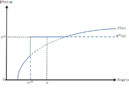
right-hand side of the constraint is the expected loss in future utility from getting caught shirking and being …red. The two constraints are depicted in Figure 1 and together form what we call the ’e¤ort function’.
Depending on the level of the wage, either the reciprocity constraint or the no-shirking constraint binds. In particular, if wt< wN S, where wN S is the wage for which the no-shirking
constraint holds with equality, the utility loss from providing eN S outweighs the expected
cost from getting caught shirking and the worker provides e¤ort eR
t < eN S according to
his reciprocity concerns (solution 1). Vice versa, if wt > wN S as drawn in the …gure, the
no-shirking constraint outweighs the reciprocity constraint and the worker provides e¤ort eN S > eR
t (solution 2). Finally, for a su¢ ciently high wage, reciprocity concerns imply an
e¤ort level eR
t > eN S in which case the no-shirking constraint becomes moot since monitored
workers are never found shirking (solution 3).
Notice that depending on functional form assumptions, we may not observe all three of the solutions. For example, if eRt exceeds eN S at wN S, solution 2 never occurs. In turn, if
eRt < eN S for any wage level, solution 3 never occurs. Also, a special but as it turns out relevant shape of the reciprocity constraint obtains if workers perceive the …rm’s payo¤ f (e; ) as increasing in e¤ort up to some e¤ort level e = ~e and constant thereafter (i.e. f0(e) = 0for
e > ~e). For this particular functional form, there still exists a unique reciprocity constraint that is increasing in the wage up to eR
t = ~e and is ‡at thereafter.8
2.2
Implications
The reciprocity constraint and the no-shirking constraint depend on the wage and the time left in the employment relationship. We now consider the implications on e¤ort of varying these two determinants, conditional on di¤erent assumptions about monitoring and reci-procity.
8To see this, note that the assumption of f0(e) = 0 for e > ~e introduces a non-di¤erentiability in
r(e; ) at e = ~e. Hence, lime!~e re(e; )g(wt) > v0(e) and optimal e¤ort from reciprocity solves v0(eR) =
re(eR; )g(w; ) for eRt < ~e and eRt = ~e thereafter. The resulting reciprocity constraint is close to the
2.2.1 No monitoring
Consider …rst a situation in which workers believe that e¤ort is not monitored (i.e. d = 0). Under the standard assumption that workers do not have reciprocity concerns (i.e. = 0), we obtain the following unambiguous prediction.
Result 1 For d = 0 and = 0, workers always supply e¤ort equal to the norm level e = 0, independent of wage changes or the time left in the employment relationship.
The intuition for this result is straightforward. If workers do not have reciprocity, eR t = 0
by assumption that the disutility of e¤ort v(e) is at its minimum at e = 0. Since v( ) does not depend on either the wage or the time left to T , et = 0 for all wt and t.
If we assume instead that workers have reciprocity concerns (i.e. > 0), the predictions of the model are radically di¤erent.
Result 2 For d = 0 and > 0:
1. An increase (decrease) in wages leads to an increase (decrease) in e¤ort. In addition, the increase in e¤ort in response to a given wage increase is strictly smaller (in absolute terms) than the decrease of e¤ort in response to a wage decrease of the same magnitude. 2. E¤ort depends negatively on past wages as long as the reference wage level w is
in-creasing in past wages.
3. E¤ort does not change as t ! T .
Result 2.1 follows directly from the concavity of the reciprocity constraint and the fact that for d = 0, the no-shirking constraint never binds. The asymmetric response of e¤ort to positive and negative wage changes has been discussed in several empirical studies (see references in introduction) but, to our knowledge, as not been formally explored to date. Also note that this asymmetry can be extreme for the special case discussed above where the reciprocity constraint becomes ‡at above a certain wage for which eR
t = ~e. In this case,
an increase in the wage does not increase e¤ort whereas a decrease in the wage may lead to lower e¤ort (provided that the wage cut is su¢ ciently large to imply eR
t < ~e).
Results 2.2 and 2.3 are also direct implications of the optimal e¤ort condition in Propo-sition 1. Together, the two results generate what Bewley (2002) calls ’wage entitlement’; i.e. that workers adapt over time to a given wage treatment, no matter how high it may be, and come to use it to assess the fairness of the …rm.9
9Without Result 2.3, we would not be able to disentangle the e¤ect of a reduction in time left in the
2.2.2 Monitoring
Now consider a situation in which workers believe that e¤ort is monitored (i.e. d > 0). Under the standard assumption that workers do not have reciprocity (i.e. = 0), the model predicts the following.
Result 3 For d > 0 and = 0:
1. An increase in the path of wages fwsgTs=t leads to an increase in e¤ort from et = 0
to et = eN S if v(0) + v(eN S) > d Vt+1E Vt+1U before the change and the resulting
increase in VE
t+1 Vt+1U is su¢ ciently large so as to revert the inequality. The exact
opposite inequality conditions have to be met for a decrease in the path of wages to lead to a decline in e¤ort from et= eN S to et= 0.
2. As t ! T , e¤ort decreases from et = eN S to et = 0 for a given wage path if v(0) +
v(eN S) d Vt+1E Vt+1U for some t < t0 < T and Vt+1E Vt+1U becomes su¢ ciently small
for some t0 < t < T such that the inequality changes sign
Both of these results are a direct application of Proposition 2 for the special case where the worker has no reciprocity concerns (in which case optimal e¤ort is 0 if the wage does not satisfy the no-shirking constraint).
If workers also have reciprocity concerns ( > 0), the general solution from Proposition 2 obtains and the model makes the following predictions.
Result 4 For d > 0 and > 0:
1. An increase in the path of wages fwsgTs=t leads to an increase in optimal e¤ort if the
reciprocity constraint is binding (i.e. solution 1 or solution 3 in Proposition 2); or if the no-shirking constraint is binding (i.e. solution 2), the resulting increase in VE
t+1 Vt+1U
is su¢ ciently large so as to make the reciprocity constraint binding. The exact opposite conditions have to be met for a decrease in the path of wages to lead to a decrease in optimal e¤ort.
2. As t ! T , e¤ort decreases from eN S to eR
t < eN S for a given wage path if the
no-shirking constraint is binding for some t < t0 < T and Vt+1E Vt+1U becomes su¢ ciently
small for some t0 < t < T such as to make the reciprocity constraint binding (i.e.
While these two results seem may complicated, they are a simple extension of Results 3 and can be easily understood by reconsidering Figure 1 for di¤erent wage levels.
Three key lessons come out of this analysis. First, absent explicit incentives (either through monitoring or other performance controls), e¤ort varies with wage changes only if workers have reciprocity concerns. Second, wage entitlement in reciprocal behavior implies that a temporary increase in the wage has a negative overall e¤ect on e¤ort. Third, the presence of explicit incentives (e.g. through a monitoring-induced …ring threat) may outweigh reciprocity concerns, thus highlighting the importance of having a measure of e¤ort that workers perceive as unmonitored when testing for reciprocity in long-term relationships.
3
Environment and experimental design
We …rst provide an overview of the environment in which the …eld experiment was conducted. Then we discuss the details of the exogenous wage changes and the measures of monitored and unmonitored e¤ort.
3.1
Environment
The experiment was conducted in the context of a household survey that took place in a rural part of Kenya in 2007. The primary purpose of the survey was not the wage experiment, but to collect socioeconomic information on participants in di¤erent community-based devel-opment projects and consisted of an average of about 900 questions per survey (depending on the size and activities of the household). The number of households to be surveyed was initially targeted at 2500 and was later extended to more than 3000, as discussed below.
To administer the surveys, the principal investigators (PIs) hired 12 members of the local community, which were selected based on a competitive interview process. The hired …eld workers were aged between 19 and 37, 7 women and 5 men, with a median age of 24. All were economically average residents, all spoke English but none had university education, and previous work experience was limited to occasional low paid employment and/or home production (e.g. farming).
Prior to the start of the survey collection, the …eld workers were invited to an extensive 4-day training camp that was organized by one of the PIs, assisted by a Kenyan student with previous survey experience and a foreign student. The two students were responsible for the supervision of the survey collection afterwards. The camp was held at a secluded lodge to ensure full focus on the training and to foster a sense of team spirit. The workers also received
a specially designed survey T-shirt and they were informed that upon successful completion of the survey collection, they would be invited to a weekend retreat to another community in Kenya. Furthermore, the PIs promised to organize a CV workshop and to provide a letter of recommendation. All of these perks were o¤ered in an e¤ort to generate a friendly and cooperative work environment that should dampen any reaction to wage changes.
After the 4-day training camp and a …nal performance assessment, the …eld workers started administering the surveys. During the …rst two weeks of work, one of the PIs was present to help the two students in supervising and …ne-tuning the survey collection. There-after, regular work (i.e. without direct presence of the PIs) started. In the beginning, …eld workers typically administered between two and three surveys per day, six days a week. Later on, as the survey collection became more e¢ ciently organized, …eld workers increased their workload to four surveys per day but were explicitly discouraged from doing more.10
3.2
Experimental design
Field workers were paid per survey. Under the initial compensation scheme, the …rst three surveys per day were paid 150 Ksh each and all subsequent surveys of the same day were paid 100 Ksh each.11 Since …eld workers administered on average between three and four
surveys per day, this implied a daily salary of about 500 Ksh –three to four times more than what a …eld worker could hope to earn elsewhere.12
During the …rst six weeks of regular employment, …eld workers were paid the just de-scribed compensation scheme, called the ’150/100 treatment’from hereon. In the beginning of work week 7, the wage rate was raised to 200 Ksh per survey (including for the fourth sur-vey of the day and beyond). This new ’200/200 treatment’represented an average increase in daily compensation of about 45% and was communicated to the …eld workers through a video announcement by the PIs. The announcement came without speci…c information on whether the raise was permanent or not. In return, the …eld workers were asked to continue administering the surveys with diligence and were reminded that they should not exceed four surveys per day.13 The new ’200/200 treatment’ continued for three weeks. In the
10For three weeks of the total employment period, …eld workers administered surveys for only 5 days. Also,
some …eld workers occasionnally exceeded and one …eld worker consistently exceeded the limit of 4 surveys per day. All of the results reported below are robust to whether we consider only the …rst four surveys per …eld worker per day; and to whether we exclude the …eld worker who consistently exceeded the limit of 4 surveys per day.
11Whenever possible, …eld workers tried to administer four surveys per day, con…rming that even 100 Ksh
per survey was well above their marginal outside option.
12At the time of the surveys, 500 Ksh were worth about US$7.4. 13The exact wording of all announcements is available in the appendix.
beginning of week 10, the two student supervisors played a second video announcement to the …eld workers in which the PIs informed them that compensation reverted back to the initial 150/100 treatment (i.e. 150 Ksh for each of the …rst three daily surveys and 100 Ksh for any additional survey). The justi…cation given for this wage cut was budget limitations that made the wage of 200 Ksh per survey unsustainable. A week later, in the beginning of week 10, a third video was played to the …eld workers in which they were informed that employment would continue for an additional three weeks so as to expand the survey beyond the initially planned 2500 households. For this extension of employment to be feasible, the workers were explained that the wage would need to be cut to 100 Ksh for each survey per day. This ’100/100 Ksh treatment’ represented an average wage cut of about 27% but it also implied that employment continued for approximately three weeks longer than initially anticipated.14 Finally, so as to avoid possible end-of-employment e¤ects, a …nal video in
the beginning of week 13 (i.e one week before the planned end of employment) informed the workers that since the target number of households had been reached, survey collection would halt immediately.15
Figure 2 summarizes the di¤erent wage treatments over the 12 weeks of regular em-ployment. Since work weeks started on Wednesdays, all video announcements about wage changes were made on Wednesday mornings before work started and took e¤ect immediately. Hence, the di¤erent work weeks in Figure 1 e¤ectively lasted from Wednesday to Tuesday. None of the videos were preanounced and, to the best of our knowledge, did not coincide with any other exceptional events. Also, at no point were the workers informed that they were taking part in an experiment.
To measure work e¤ort, we consider two di¤erent types of errors for each survey. The …rst type of error we consider is ’inconsistencies’ across di¤erent answers of a survey. An inconsistency occurred if, for example, a respondent answered in the occupation section of the survey that he/she was not farming but indicated in the time-use section that he/she spent time farming. In total, there were 93 possible inconsistencies per survey (see the ap-pendix for the full list). Field workers were made aware of the possibility of inconsistencies during training (without knowing about the 93 possibilities) and were instructed to pause the interview if they spotted an inconsistency and probe the respondent in order to resolve the problem. However, the supervisors never monitored or punished in any way for
incon-14The announcement also reassured the …eld workers that the planned post-survey weekend retreat and CV
workshop was still on regardless of participation in the extra surveys. All …eld workers continued employment to the end even though they were free to quit at any time; and all of them joined the promised post-survey retreat and participated in the CV workshop.
15Field workers continued to be paid 400 Ksh per day for the last week without work so as to honor the
sistencies, nor did anyone know that we would compute such a measure ex-post. In fact, we drew up the list of 93 possible inconsistencies and computed the rate of inconsistencies per survey via a computer algorithm only more than a year later after the di¤erent survey answers had been manually entered into a database. For all means and purposes of this ex-periment, inconsistencies therefore constitute a measure of e¤ort that …eld workes perceived as unmonitored.
The second type of errors we consider is ’blanks and mistakes’and occurred if a survey …eld was either left blank (e.g. the …eld worker forgot to ask/pencil in the question or the respondent refused to answer) or the …eld contained a clear mistake (e.g. reporting zero households in the visited homestead). In contrast to inconsistencies, …eld workers were explicitly trained to avoid these blanks and mistakes, possibly insisting with the respondents on an answer, and the two students supervisors checked incoming surveys randomly each day for these errors (between 40% and 100% of the surveys were checked each day, depending on the time available). We therefore label blanks and mistakes as ’monitored errors’. If a survey contained too many blanks and mistakes, the …eld worker was given a warning and, in case of repeated subpar performance, risked dismissal. This threat of dismissal was real. In fact, during the …rst two weeks of employment, one …eld worker consistently made numerous avoidable mistakes. Despite further extensive training, performance did not improve, and the …eld worker was subsequently laid o¤.
3.3
Discussion
As emphasized in the introduction and formalized by the model in the previous section, the long-term nature of the wage experiment implies that …eld workers had an explicit incentives to perform well on monitored dimensions of e¤ort so as not to loose their job. The availability of an e¤ort dimension that was truly unmonitored in the eyes of the worker is therefore crucial to test for reciprocity. Our inconsistency measure …ts this criteria. Hence, under the standard assumption that workers do not have reciprocity concerns, inconsistencies should be distributed randomly and unrelated to wage changes. If we …nd instead that inconsistencies change systematically with wage changes, then this represents prima facie evidence in favor of reciprocal behavior.
4
Basic results
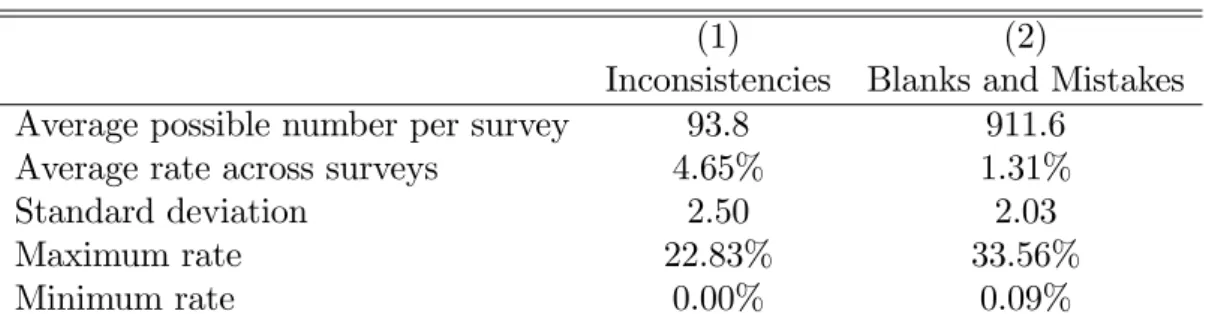
unmon-the total of 2864 administered surveys during unmon-the 12 weeks of regular employment, unmon-there was an average 4.65 percent of inconsistencies per survey (out of an average of 93.8 possible inconsistencies per survey). This is considerably higher than the average rate of blanks and mistakes of 1.31 percent per survey (out of an average of 911.6 possible blanks and mistakes per survey).
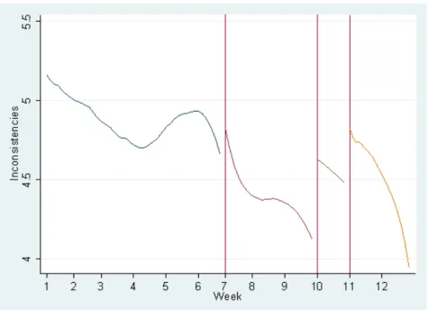
As the standard deviations and extreme values in Table 1 indicate, there is considerable variation in the two e¤ort measures. Closer inspection reveals that a substantial part of this variation is idiosyncratic and not systematically associated with particular …eld workers or time in the employment relationship. To show the general evolution of inconsistencies and blanks and mistakes, we therefore use local linear regressions to smoothen out this idiosyn-cratic variation. In addition, to foreshadow our results below, we impose a discontinuity at the days when the changes in wage treatment occurred (i.e. in the beginning of work weeks 7, 10 and 11).16 Figures 3 and 4 display the result. Three basic observations stand out:
1. There is a clear secular downward trend in the rate of inconsistencies. By contrast, the rate of blanks and mistakes is trending upwards (abstracting from the …rst two weeks). This suggests that throughout the employment, …eld workers accumulated experience in detecting and resolving inconsistencies whereas for blanks and mistakes, this learning-by-doing e¤ect was present only in the beginning or was outweighed later on by other e¤ects, as discussed below.
2. Inconsistencies jump up substantially in the beginning of weeks 10 and 11 when the two wage cuts took place. Interestingly, there is also a small positive jump in inconsistencies at the beginning of week 7 when the wage increase was administered.
3. Blanks and mistakes also display jumps around the wage change days. But these jumps are generally smaller and always negative.
While instructive, this visual inspection does not tell us whether any of the jumps are signi…cant, nor does it indicate (by construction) whether there are important jumps for weeks when no wage changes took place. To assess these issues formally, we proceed by testing econometrically for jumps at the beginning of each workweek (i.e. each Wednesday).
16The discontinuities are imposed by estimating the local linear regressions separately on each side of the
days when a wage change occured. The idea to smoothen noisy data with local linear regressions around discrete cut o¤s is taken from the literature on regression discontinuity designs (see Imbens and Lemieux, 2007 for a survey). The local linear regressions are computed in STATA using an Epanechnikov kernel. Somewhat more variable plots but with exactly the same qualitative features would have obtained with other kernels or if we had applied a simple moving average to the data.
First, we reduce some of the idiosyncratic variation by purging the two e¤ort measures of survey-speci…c e¤ects as described and estimated in the panel regressions of the next section.17 Then we compute the di¤erence between the 3-day average of the resulting residual
e¤ort measures immediately preceding the beginning of the workweek and the corresponding 3-day average starting with the beginning of the workweek. Finally, to conduct inference, we compute the bootstrapped 90% con…dence interval of the di¤erences.
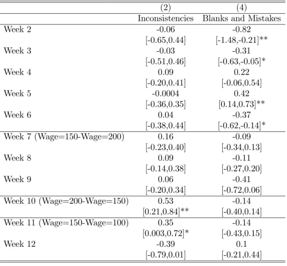
Table 2 displays the results. As column (1) shows, the rate of inconsistencies increases signi…cantly by 0.53 percentage points and 0.35 percentage points, respectively, in the be-ginning of week 10 and week 11 when the wage cuts were administered. Relative to the average rate of inconsistencies of 4.65 percent per survey, this represents an increase of 11.3 percent and 7.5 percent, respectively. By contrast, there is no signi…cant change for any of the other weeks. In particular, in the beginning of week 7 when the wage was increased, inconsistencies do not react signi…cantly. Column (2) shows the corresponding results for the rate of blanks and mistakes. While there are several signi…cant changes during the …rst 6 weeks, there are no signi…cant changes thereafter. Importantly, in the beginning of weeks 7, 10 and 11, the rate of blanks of mistakes essentially remains ‡at.
Four key implications come out of these results. First, the signi…cant increase in the rate of inconsistencies in the beginning of weeks 10 and 11 when wages are cut provides clear evidence of negative reciprocity. As implied by Results 1 and 2 of our model, unmoni-tored e¤ort reacts systematically to wage changes only if workers have reciprocity concerns. Speci…cally, a wage cut signals a smaller gift by the …rm to which workers react with reduced e¤ort. By contrast, there are no positive reciprocity e¤ects in response to the wage increase in the beginning of week 7. As discussed towards the end of Section 2, such an extreme asymmetry is consistent with the model if the reciprocity constraint becomes ‡at above a certain wage level. This can occur if the initial wage-e¤ort equilibrium is already so high that, in the workers’ minds, additional e¤ort in response to an even higher wage does not lead to a further increase in the psychological bene…ts from reciprocating. Given that the initial 150/100 treatment amounted to a daily compensation that was three to four times higher than the going market compensation, this is a distinct possibility. By the same token, the generous initial treatment makes the decrease of unmonitored e¤ort in response to the wage cuts all the more striking – especially since the PIs went to great lengths to foster a cooperative work environment and the wage cuts were framed as necessary to respect budget limitations.
17These survey-speci…c e¤ects are a …eld worker …xed e¤ects; a gender of the respondent control; a
Second, the absence of a signi…cant drop in inconsistencies in the beginning of week 7 together with the presence of a signi…cant increase in inconsistencies in week 10 when the wage was lowered back to the original 150/100 treatment suggests that workers adapted quickly to the higher 200/200 treatment from week 7 to week 10 and came to believe that this was the new reference against which a given wage o¤er should be judged. As implied by Results 2.2 and 2.3 of our model, this wage entitlement e¤ect is a potentially important source of asymmetric reciprocity behavior. At the same time, the local discontinuity tests that we perform in Table 2 do not allow us to separate the e¤ects of wage entitlement from secular time trends in inconsistencies as observed in Figure 3. The panel estimation that we perform in the next section allows us disentangle these two temporal phenomena from each other.
Third, the absence of any signi…cant response of blanks and mistakes to the di¤erent wage changes in the beginning of week 7, 10 and 11 suggests that monitoring imposed an important additional constraint that outweighed …eld workers’negative reciprocity behavior. Speci…cally, recall from Result 4 of the model that a decrease in wages only leads to a decrease in monitored e¤ort (i.e. an increase in blanks and mistakes) if either the no-shirking constraint is not binding before the wage decrease or the wage decrease is su¢ ciently large for the reciprocity constraint to replace the no-shirking constraint as the binding constraint. The absence of a signi…cant reaction in blanks and mistakes to the two wage cuts therefore implies that the no-shirking constraint was binding not only at the initial 150/100 treatment but also at the lower 100/100 treatment, which seems plausible given the limited outside options of the workers.
Fourth, the …nding of negative reciprocity for inconsistencies implies that the presence of explicit incentives does not necessarily crowd out reciprocal behavior, as suggested by certain laboratory experiments (e.g. Fehr and Gächter, 2000b).18 Otherwise, workers would
have provided minimal e¤ort on resolving inconsistencies throughout the entire experiment. A possible concern about the results in Table 2 is that reciprocal behavior is irrelevant and that inconsistencies increased instead because of some idiosyncratic shocks that coincided with the wage cuts in the beginning of weeks 10 and 11. Several reasons speak against this possibility. First and most importantly, if inconsistencies had increased because of some large idiosyncratic shock (e.g. inclement weather, uncooperative survey respondents), one would expect to see the same shock to also increase the rate of blanks and mistakes. This is clearly not the case.19 Second, as described above, the estimates in Table 2 control for
18More speci…cally, this crowding out argument means that reciprocity concerns simply disappear (i.e.
= 0 in our model) if …rms impose explicit incentives.
di¤erent survey-speci…c e¤ects. Third, the wage changes were implemented on Wednesdays, in the middle of the regular week, on otherwise uneventful days. Closer inspection of the data reveals, moreover, that the …eld workers’behavior did not change noticeably in other dimensions (e.g. the time used per survey or the average number of surveys administered per day). Fourth, as Figure 3 shows, the signi…cant increases in inconsistencies in the beginning of weeks 10 and 11 were not the result of a strong positive secular time trend due, for example, to fatigue e¤ects. In fact, exactly the opposite is true: throughout the entire employment relationship, the rate of inconsistencies exhibited a marked downward trend, interrupted only by the jumps in response to the wage cuts. For all these reasons, it seems highly unlikely that our results are driven by events other than the exogenous wage changes.
5
Panel estimates
To assess the e¤ect of wage changes further, we perform panel estimations on the full dataset. The use of the entire dataset instead of just data around particular days increases power and allows us to directly control for secular time trends.
5.1
Econometric speci…cation
The panel regressions take the form
eijt = j+ Dwage+ Xijt+ 1t + 2t2+ uijt, (7)
where i identi…es the survey; j the …eld worker; and t the survey day. The dependent variable eijt is alternatively the rate of inconsistencies or the rate of blanks and mistakes for
a given survey. The coe¢ cient j captures …xed worker e¤ects; Dwage is a vector of dummy
variables for each of the wage regimes (described in detail below); and Xijt represents a set
of observable non-wage controls that may change systematically across surveys, …eld workers and time.20 The term 1t+ 2t2 captures secular trends due for example to learning-by-doing
as observed for inconsistencies in Figure 3. We specify this trend in quadratic form so as to provide the estimation with ‡exibility to accommodate e¤ects that are either slowly dying out over time or manifest themselves only over time. As shown below, the results are robust to other forms of the time trend. Note also that this time trend is identi…ed separately from
remained constant. By contrast, inconsistencies did not change signi…cantly during these …rst six weeks. This suggests that blanks and mistakes are more sensitive to idiosyncratic shocks than inconsistencies.
20Speci…cally, X
the wage dummies in Dwage because we make it a function of survey day t. Finally, uijt
denotes an uncorrelated error term.
The key coe¢ cients of interest are contained in the vector and measure the e¤ect that the di¤erent wage dummies in Dwage have on the error rate in question. In de…ning
these dummies, we face a choice of time interval per dummy. We choose to de…ne one separate dummy per week. This is a natural benchmark because all wage changes occurred on Wednesdays and because it provides a good trade-o¤ between sample size and su¢ ciently small time intervals to capture the discontinuity around the wage changes.21 To identify the
e¤ect of each dummy on eijt, we de…ne week 6 as the reference, which is the last week of
the initial 150/100 treatment before the increase to the 200/200 treatment. Vector Dwage
therefore contains eleven dummies taking on the value of 1 for the respective week and 0 otherwise; and the di¤erent coe¢ cients in = [ 1; ::: 5; 7; ::: 12]capture the impact of each week relative to the omitted reference week 6. Remembering the timing of the wage changes described in Figure 2, 7 captures the impact on eijt of the 200/200 treatment in week 7,
as opposed to the 150/100 treatment during reference week 6; 10 captures the impact of returning to the 150/100 treatment in week 10 relative to the initial 150/100 treatment during the reference period in week 6; and so forth.
5.2
Estimates
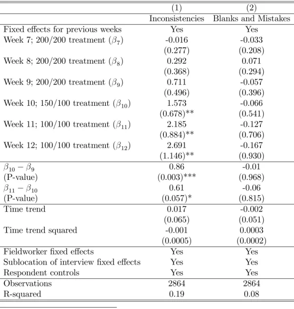
Column (1) of Table 3 displays the results for inconsistencies. Robust standard errors are reported in parentheses below each estimate. There is no signi…cant di¤erence in inconsisten-cies between the reference week and the …rst …ve weeks, where compensation is at the initial 150/100 treatment (for space reasons, we do not report these coe¢ cients). The …rst three coe¢ cients ( 7 to 9) capture the e¤ect on inconsistencies of the increase in compensation to the 200/200 treatment in weeks 7 to 9. None of these e¤ects are signi…cant. By contrast, the last three coe¢ cients ( 10 to 12) show that relative to the initial 150/100 treatment during the reference period in week 6, the rate of inconsistencies jumps signi…cantly as the wage …rst returns to the original 150/100 treatment in week 10 and then jumps further as compensation is lowered to the 100/100 treatment in weeks 11 and 12. In addition, as the positive and signi…cant di¤erence in coe¢ cients 10 9 and 11 10 indicates, the increase
in inconsistencies is signi…cant not only with respect to the reference period in week 6 but also with respect to the weeks directly preceding the wage cuts.
These estimates fully con…rm the basic results of Table 2. Speci…cally, the estimate for
7 is insigni…cant whereas the di¤erences 10 9 and 11 10 are positive and signi…cant.
These two di¤erences are somewhat larger than the estimates for weeks 10 and 11 in Table 2, representing an increase of 18.5 percent and 13.1 percent in the rate of inconsistencies relative to the average rate of 4.65 percent. The larger magnitude of these estimates is due to the fact that the panel estimation considers weekly intervals rather than 3-day intervals and includes a time trend. In line with the overall evolution of inconsistencies displayed in Figure 2, this time trend is estimated to be negative except for the very beginning of the employment relationship (i.e. the negative quadratic term quickly overpowers the positive linear term), presumably capturing a learning-by-doing e¤ect.
The inclusion of a time trend allows us to separately identify the e¤ects of wage enti-tlement and is captured by the large and signi…cant point estimate 10 of 1.573 percentage points. Relative to the average rate of inconsistencies of 4.65 percent, this estimate repre-sents a jump of 34 percent and measures the impact of returning to the 150/100 treatment in week 10 relative to the same 150/100 treatment in reference week 6. Workers therefore appear to have quickly adapted to the 200/200 treatment in weeks 7 to 9 and considered this as the new norm even though the daily compensation implied by this treatment was several times higher than any available outside options. This …nding o¤ers direct support for Bew-ley’s (2002) conclusion from interviews with managers and labor leaders that "...employees usually have little notion of a fair or market value for their services and quickly come to believe that they are entitled to their existing wage, no matter how high it may be..." (page 7).
Column (2) of Table 3 shows that none of the wage changes has a signi…cant e¤ect on the rate of blanks and mistakes, con…rming again the basic results of Table 2. Furthermore, most of the signi…cant jumps in weeks 1-4 now disappear (not shown for space reasons). The absence of signi…cant results for blanks and mistake in weeks 10 and 11 indicates one more time that the large and signi…cant response of inconsistencies to wage cuts are not driven by some random coincident events. Instead, the results in Column (2) suggest that the presence of explicit incentives through monitoring outweighed the …eld workers’negative reciprocity behavior.
5.3
Robustness
To provide additional support for our results, we perform several robustness checks. Table 4 reports results from exploiting the particular wage structure during the 150/100 treatment and the 100/100 treatment. The …rst row tests whether, during weeks 1 to 6 when the initial
e¤ort of wage changes within each day. As the estimates show there is no signi…cant di¤erence in either e¤ort measure between the third survey (paid 150 Ksh) and the fourth survey and beyond (paid 100 Ksh). Hence, the negative reciprocity e¤ects found for wage changes across time in Table 3 do not apply to wage changes within each day. This suggests that workers’ reciprocity depends on changes in the wage contract as opposed to the details of a given contract, lending further support to Bewley’s (2002) conclusion that employees have little notion of a fair or market value in absolute terms.
Rows 2 to 6 of Table 4 checks the robustness of our main results in Table 3 by using only the …rst three surveys for each day. All results are con…rmed: (i) there is no signif-icant reaction of inconsistencies in week 7 when the wage per survey is increased to the 200/200 treatment; (ii) inconsistencies increase signi…cantly as the wage returns to the base-line 150/100 treatment in week 10; (iii) inconsistencies increase even further as the wage drops to the 100/100 treatment in week 11; and (iv) there is no signi…cant reaction in blanks and mistakes for any of the wage changes.
The last row of Table 4, …nally, shows that there is also a strong and signi…cant increase in inconsistencies for the …rst three surveys per day in week 11, paid 100 Ksh each, relative to the fourth survey per day in weeks 1 to 6 even though this fourth survey was paid the same 100 Ksh and was administered at the end of the day. This test provides further con…rmation of the wage entitlement e¤ect discussed above.
Table 5 goes through a battery of additional robustness checks for the panel regressions on inconsistencies in Table 3. Column (1) repeats the baseline estimation of Column (1) in Table 3. Columns (2) and (3) show that none of the results change when (i) the reference week is changed to week 5; and (ii) the two training weeks prior to the regular work relationship are included (the weeks when one of the PIs was present). Columns (4) to (6) show that the results are also robust to (i) omission of respondent controls; (ii) omission of sublocation …xed e¤ects; and (iii) replacement of the quadratic time trend with a linear time trend (now estimated to be negative, consistent with Figure 2).22 Lastly, as discussed above, since wage changes were enacted on a weekly basis, a week is the natural choice of time interval per dummy. A more re…ned but less powerful analysis at a 3 day level, where Wednesday-Thursday-Friday would form a …rst block, and Saturday-Monday-Tuesday another (workers took Sunday o¤), leads to essentially similar results.23
22Likewise, the results are robust to the inclusion of a cubic time trend. 23Results available upon request.
6
Conclusion
This paper tests for reciprocity in labor relations using a …eld experiment in an actual labor market. The novelty of our paper relative to existing …eld experiments in this literature is that we devised a measure of e¤ort that workers perceived as truly unmonitored. This allowed us to follow the same workers over an extended period of time and estimate how their reciprocal behavior responded to a sequence of wage raises and wage cuts. The two main results coming out of our experiment is that (i) workers exhibited negative reciprocity with respect to wage cuts but no positive reciprocity with respect to wage raises; and that (ii) workers quickly adapted to a new higher reference wage when deciding on the reci-procity response to a given wage o¤er. Our analysis also reveals that explicit incentives on monitored dimensions of e¤ort can easily outweigh the e¤ects of reciprocity; but that the presence of explicit incentives in itself does not necessarily crowd out the workers propensity to reciprocate.
These results may help understand a number of important labor market phenomena. In particular, as Collard and De la Croix (2000) and Danthine and Kurmann (2004, 2010) show in a dynamic general equilibrium context, the assumption of wage entitlement is crucial for reciprocity-based e¢ ciency wage models to generate endogenous wage rigidity and for rela-tively small shocks to imply large and persistent business cycle ‡uctuations. Furthermore, the asymmetric response of unmonitored e¤ort to wage cuts relative to wage increases pro-vides an explanation for the lack of wage cuts (i.e. downward wage rigidity) observed in many micro wage data sets of industrialized countries (e.g. Dickens et al., 2007). As Bew-ley (1999) argues: "...resistance to pay reduction comes primarily from employers, not from workers or their representatives, though it is anticipation of negative employee reactions that makes employers oppose pay cutting. The claim that wage rigidity gives rise to unexploited gains from trade is invalid, because a …rm would lose more money from the adverse e¤ects of cutting pay than it would gain from lower wages and salaries." (page 430-31). Viewed in this way, this …eld experiment represents a counterfactual of what a …rm should not do, with the negative reaction of workers to the wage cuts con…rming Bewley’s point.
References
[1] Agell, J. and P. Lundborg, 1995. Theories of pay and unemployment: survey evidence from Swedish manufacturing …rms. Scandinavian Journal of Economics 97, 295— 307. [2] Agell, J. and P. Lundborg, 1999. Survey evidence on wage rigidity: Sweden in the 1990s.
FIEF Working Paper 154.
[3] Akerlof, G., and J. Yellen, 1990. The Fair-Wage E¤ort Hypothesis and Unemployment. Quarterly Journal of Economics, 105 (1990), 255-283.
[4] Akerlof, G. A., 1982. Labor Contracts as Partial Gift Exchange. Quarterly Journal of Economics, 97, 543- 569.
[5] Bandiera, Oriana, Iwan Barankay, and Imran Rasul, 2005. Social Preferences and the Response to Incentives: Evidence from Personnel Data. Quarterly Journal of Economics, 120(3): 917–62.
[6] Bellemare, C., and B. Shearer, 2009. Gift Giving and Worker Productivity: Evidence from a Firm Level Experiment. Games and Economic Behavior, vol. 67, pp. 233-244 [7] Bewley, T. F., 1999. Why Wages Don’t Fall During a Recession. Cambridge: Harvard
University Press.
[8] Bewley, T. F., 2002. Fairness, Reciprocity, andWage Rigidity. Cowles Foundation Dis-cussion Paper No. 1383.
[9] Blinder, A. S., and D. H. Choi, 1990. A Shred of Evidence on Theories of Wage Sticki-ness. The Quarterly Journal of Economics, 105 (1990), 1003-1015.
[10] Campbell, C., Kamlani, K., 1997. The Reasons for Wage Rigidity: Evidence from Survey of Firms. Quarterly Journal of Economics, 112, 759-789.
[11] Charness, G., G. R. Frechette, and J. H. Kagel, 2004. How Robust Is Laboratory Gift Exchange? Experimental Economics, 7 (2004), 189-205.
[12] Charness, G., and P. Kuhn, 2007. Does Pay Inequality A¤ect Worker E¤ort? Experi-mental Evidence. Journal of Labor Economics, 25 (2007), 693-723.
[13] Charness, G., and M. Rabin, 2002. Understanding Social Preferences With Simple Tests. The Quarterly Journal of Economics, MIT Press, vol. 117(3), pages 817-869, August.
[14] Cohn, A., E. Fehr, and L. Goette, 2009. Fair Wages and E¤ort: Evidence from a Field Experiment. IEW Working Paper, University of Zurich, 2009.
[15] Cohn, A., E. Fehr, B. Herrmann, and F. Schneider, 2011. Social Comparison in the Workplace: Evidence from a Field Experiment. IZA Discussion Papers 5550, Institute for the Study of Labor (IZA)
[16] Collard, F., De la Croix, D., 2000. Gift Exchange and the Business Cycle: The Fair Wage Strikes Back. Review of Economic Dynamics, 3, 166-193.
[17] Danthine, J.-P. and A. Kurmann, 2010. The Business Cycle Implications of Reciprocity in Labor Relations. Journal of Monetary Economics, vol. 57(7), 837-850.
[18] Danthine, J.-P. and A. Kurmann, 2008. The Macroeconomic Consequences of Reci-procity in Labor Relations. Scandinavian Journal of Economics, vol. 109(4), 857-881. [19] Danthine, J. P., Kurmann, A., 2004. Fair Wages in a New Keynesian Model of the
Business Cycle. Review of Economic Dynamics, 7, 107-142.
[20] Dickens, W., Goette, L., Groshen, E., Holden, S., Messina, J., Schweitzer, M., Turunen, J., and M. Ward, 2007. How Wages Change: Micro Evidence from the International Wage Flexibility Project. Journal of Economic Perspectives, Volume 21, N.2, Spring 2007, Pages 195–214.
[21] Falk, Armin & Fischbacher, Urs, 2006. A theory of reciprocity. Games and Economic Behavior, Elsevier, vol. 54(2), pages 293-315, February.
[22] Fehr, Ernst, Georg Kirchsteiger, and Arno Riedl. 1993. Gift Exchange and Ultima-tum in Experimental Markets. Vienna Economics Papers vie9301, University of Vienna, Department of Economics
[23] Fehr, E., S. Gächter and G. Kirchsteiger, 1997. Reciprocity as a Contract Enforcement Device. Econometrica 65, 833-860.
[24] Fehr, E. and A. Falk, 1999. Wage Rigidity in a Competitive Incomplete Contract Market. Journal of Political Economy, 107, 106-134.
[25] Fehr, E. and S. Gächter, 2000a. Fairness and Retaliation: The Economics of Reciprocity. Journal of Economic Perspectives, 14, 159-181.
[26] Fehr, Ernst and Simon Gächter, 2000b. “Do Incentive Contracts Crowd-Out Voluntary Cooperation? Working paper No 34, Institute for Empirical Research in Economics, University of Zurich.
[27] Gneezy, U., and J. List, 2006. Putting Behavioral Economics to Work: Field Evidence of Gift Exchange. Econometrica, 74 (2006), 1365-1384.
[28] Hannan, R. L., J. H. Kagel, and D. V. Moser, 2002. Partial Gift Exchange in an Exper-imental Labor Market: Impact of Subject Population Di¤erences, Productivity Di¤er-ences, and E¤ort Requests on Beha. Journal of Labor Economics, 20 (2002), 923-951. [29] Imbens, G.W., Lemieux, T., Regression discontinuity designs: A guide to practice,
Journal of Econometrics (2007
[30] Kahneman, D., Knetsch, J. L., Thaler, R., 1986. Fairness as a Constraint of Pro…t Seeking: Entitlements in the Market. American Economic Review, 76, 728-241.
[31] Kim, Min Taec and Robert Slonim, 2010. The e¤ect of the gift exchange with multidi-mensional e¤ort: Evidence from a hybrid …eld-lab experiment.
[32] Kube, S., M. Maréchal, and C. Puppe, 2010. Do Wage Cuts Damage Work Morale? Evidence from a Natural Field Experiment. IEW Working Paper, University of Zurich Working Paper No. 471.
[33] Rabin, M., 1993. Incorporating Fairness into Game Theory and Economics. American Economic Review, 83, 1281-1302.
[34] Rotemberg, J., 2006. Altruism, Reciprocity and Cooperation in the Workplace, in Serge Christophe Kolm and Jean Mercier Ythier, eds., Handbook on the Economics of Giving, Reciprocity and Altruism, vol. 2, North Holland, pp 1371-1407.
[35] Shapiro, C., Stiglitz, J. E., 1984. Equilibrium Unemployment as a Worker Discipline Device. American Economic Review, 74, 433-444.
[36] Solow, R. M., 1979. Another Possible Source of Wage Rigidity. Journal of Macroeco-nomics, 1, 79-82.
[37] Williamson, Oliver E., 1985. The Economic Institutions of Capitalism: Firms, Markets, Relational Contracting. New York, Free Press, 1985.
Figure 1: The e¤ort function
Figure 3: Average rate of inconsistencies (smoothed by local linear regression with Epanechnikov kernel)
Figure 4: Average rate of blanks and mistakes (smoothed by local linear regression with Epanechnikov kernel)
Table 1: descriptive statistics
(1) (2)
Inconsistencies Blanks and Mistakes
Average possible number per survey 93.8 911.6
Average rate across surveys 4.65% 1.31%
Standard deviation 2.50 2.03
Maximum rate 22.83% 33.56%