HAL Id: hal-01806200
https://hal.archives-ouvertes.fr/hal-01806200
Submitted on 17 Sep 2020
HAL is a multi-disciplinary open access
archive for the deposit and dissemination of
sci-entific research documents, whether they are
pub-lished or not. The documents may come from
teaching and research institutions in France or
abroad, or from public or private research centers.
L’archive ouverte pluridisciplinaire HAL, est
destinée au dépôt et à la diffusion de documents
scientifiques de niveau recherche, publiés ou non,
émanant des établissements d’enseignement et de
recherche français ou étrangers, des laboratoires
publics ou privés.
combination of in situ measurements, satellite data, and
atmospheric general circulation modeling
You He, Camille Risi, Jing Gao, Valérie Masson-Delmotte, Tandong Yao,
Chun-Ta Lai, Yongjian Ding, John Worden, Christian Frankenberg, Hélène
Chepfer, et al.
To cite this version:
You He, Camille Risi, Jing Gao, Valérie Masson-Delmotte, Tandong Yao, et al.. Impact of
atmo-spheric convection on south Tibet summer precipitation isotopologue composition using a
combina-tion of in situ measurements, satellite data, and atmospheric general circulacombina-tion modeling. Journal
of Geophysical Research: Atmospheres, American Geophysical Union, 2015, 120 (9), pp.3852 - 3871.
�10.1002/2014JD022180�. �hal-01806200�
RESEARCH ARTICLE
10.1002/2014JD022180Special Section:
Key Points:
• Upstream convection controls isotopic composition • Isotopic composition is more
influenced by encountered convection
• Condensation over foothill is the most important process
Correspondence to:
J. Gao,
JingGao@itpcas.ac.cn
Citation:
He, Y., et al. (2015), Impact of atmospheric convection on south Tibet summer precipitation iso-topologue composition using a combination of in situ measure-ments, satellite data and atmospheric general circulation modeling, J. Geo-phys. Res. Atmos., 120, 3852–3871, doi:10.1002/2014JD022180.
Received 23 JUN 2014 Accepted 1 APR 2015
Accepted article online 7 APR 2015 Published online 11 MAY 2015
©2015. American Geophysical Union. All Rights Reserved.
Impact of atmospheric convection on south Tibet
summer precipitation isotopologue composition
using a combination of in situ measurements,
satellite data, and atmospheric general
circulation modeling
You He1,2,3, Camille Risi3, Jing Gao2,4, Valérie Masson-Delmotte5, Tandong Yao2,4, Chun-Ta Lai6,
Yongjian Ding1, John Worden7, Christian Frankenberg7, Helene Chepfer3, and Gregory Cesana3
1Cold and Arid Regions, Environmental and Engineering Research Institute, Chinese Academy of Sciences, Beijing, China, 2Key Laboratory of Tibetan Environment Changes and Land Surface Processes, Institute of Tibetan Plateau Research,
Chinese Academy of Sciences, Beijing, China,3Laboratoire de Météorologie Dynamique, Institut Pierre Simon Laplace,
CNRS, Paris, France,4CAS Center for Excellence in Tibetan Plateau Earth Sciences, Chinese Academy of Sciences, Beijing,
China,5Laboratoire des Sciences du Climat et de l’Environnement /Institut Pierre Simon Laplace (UMR CEA CNRS UVSQ
8212), Gif-sur-Yvette, France,6Department of Biology, San Diego State University, San Diego, California, USA, 7Jet Propulsion Laboratory, California Institute of Technology, Pasadena, California, USA,
Abstract
Precipitation isotopologues recorded in natural archives from the southern Tibetan Plateau may document past variations of Indian monsoon intensity. The exact processes controlling the variability of precipitation isotopologue composition must therefore first be deciphered and understood. This study investigates how atmospheric convection affects the summer variability of𝛿18O in precipitation (𝛿18Op) and 𝛿D in water vapor (𝛿Dv) at the daily scale. This is achieved using isotopic data from precipitation samples at
Lhasa, isotopic measurements of water vapor retrieved from satellites (Tropospheric Emission Spectrometer (TES), GOSAT) and atmospheric general circulation modeling. We reveal that both𝛿18O
pand𝛿Dvat Lhasa
are well correlated with upstream convective activity, especially above northern India. First, during days of strong convection, northern India surface air contains large amounts of vapor with relatively low𝛿Dv.
Second, when this low-𝛿Dvmoisture is uplifted toward southern Tibet, this initial depletion in HDO is further
amplified by Rayleigh distillation as the vapor moves over the Himalayan. The intraseasonal variability of the isotopologue composition of vapor and precipitation over the southern Tibetan Plateau results from these processes occurring during air mass transportation.
1. Introduction
The isotopologues of precipitation (HDO and H18
2O) stored in natural archives have long been used for paleo-climate reconstructions [Dansgaard et al., 1969; Jouzel et al., 1987; Yao et al., 1996]. The Tibetan Plateau (TP) and its surrounding areas contain the largest number of glaciers outside polar regions, from which ice cores can be extracted and analyzed. However, the exact climatic controls on the isotopologue composition of precipi-tation on the TP remain debated. This makes the climatic interpreprecipi-tation of isotopologue variations recorded in Tibetan ice cores and other archives uncertain at interannual, decadal, or paleoclimatic time scales. The relative abundances of isotopologues in water samples are quantified by the equation:𝛿 = 1000 × (Rsample∕RVSMOW− 1) and they are expressed in per mil. Rsampleis the abundance ratio of the heavy to light isotopologue in a sample, and RSMOWis the abundance ratio of the heavy to light isotopologue in VSMOW water (Vienna standard mean ocean water). VSMOW is characterized by a D∕H ratio of 155.76 × 10⁻⁶and a 18O∕16Oratio of 2005.2 × 10−6.
Several factors can affect the isotopologue composition of water vapor and precipitation over the TP. The “temperature effect,” i.e., a positive local correlation between temperature and heavy isotopologue compo-sition in precipitation (𝛿18O
p), has been widely documented, especially in the northern TP [Yao et al., 1996; Tian et al., 2001a; Yu et al., 2008], and early interpretations of Tibetan ice cores were focused on temperature
[Thompson, 2000]. In the southern part of the TP, in contrast, the “amount effect,” i.e., a negative correlation
Fast Physics in Climate Models: Parameterization, Evaluation and Observation
between local precipitation amount and𝛿18O
p, has been documented [Tian, 2003]. Relationships with
pre-cipitation amount can also be nonlocal and involve upstream effects. Several studies have highlighted the important role of convective activity along air mass trajectories in various monsoon regions: Asia [Vuille et al., 2005; Schmidt et al., 2007; LeGrande et al., 2009; Lee et al., 2012; Gao et al., 2013], Western Africa [Risi et al., 2008a, 2008b; Tremoy et al., 2012] and South America [Vimeux et al., 2005, 2011; Samuels-Crow et al., 2014]. Moreover, changes in moisture sources and transport paths are also known to affect TP precipitation isotopologue composition [Araguas-Araguas et al., 1998; Aggarwal et al., 2004; Jouzel et al., 2013], and specifically the relative contributions of moisture transported by westerlies or Indian monsoon flow [Yao et al., 2013].
The goal of this study is to better understand what controls the isotopologue composition of precipitation recorded in Southern Tibetan ice cores. As a first step, we focus here on understanding the climatic controls on𝛿18O
pat the daily scale. We expect isotopologue variations at the daily scale to reflect atmospheric
pro-cesses in a more straightforward way than at longer time scales. The signal archived in ice cores arises from the accumulation of precipitating events which therefore integrate synoptic or intraseasonal phenomena. Lhasa (29.70◦N, 91.13◦E), where continuous and long-term precipitation isotopologue composition (𝛿18O
p)
moni-toring has been operational since 1996 [Tian et al., 2001a; Tian, 2003; Gao et al., 2011, 2013; Yao et al., 2013], was selected as a representative site of the southern TP where summer (June-July-August-September; JJAS) climate is primarily under the influence of the Indian summer monsoon [Yao et al., 2012; Mölg et al., 2014]. Understanding the processes controlling the variability of Lhasa precipitation isotopologue composition may also shed new light on the interpretation of nearby ice core records, such as those drilled at Zhadang (30.50◦N, 90.65◦E) and Gurenhejou (30.19◦N, 90.46◦E) [Yu et al., 2013]. A recent classification of TP glaciers based on very high-resolution reanalysis products and calculation of seasonality of precipitation/accumulation concludes that glaciers from south to central Tibet, near Lhasa are unequivocally dominated by summer precipitation (more than 60% from JJA) [Fabien et al., 2014]. Lhasa is located at an elevation of 3685 m above sea level, with an average summer temperature of 12◦C. We focus here on the summer season, from June to September, which accounts for 85% of annual southern TP precipitation [You et al., 2012]. The annual mean precipitation amount is 400 mm from 1997 to 2007.
Precipitation samples at Lhasa were collected at event scale during 3 years (2005–2007). Statistical analyses of this data set revealed that the intrasummer variability of Lhasa𝛿18O
pis closely related to the variability of
upstream convection in northern India, several days prior to the precipitation event [Gao et al., 2013]. Here in order to understand the mechanisms relating upstream convection and𝛿18O
p, we complement this data set
with remote sensing data which allow us to investigate the evolution of water vapor isotopologue composi-tion (𝛿Dv) along air mass trajectories. The isotopologue composition of water vapor provides key information:
(1) vapor is observed more continuously in space and time than precipitation, which is only sampled dur-ing precipitation events; (2) unlike precipitation, it is less affected by postcondensational processes such as reevaporation of falling droplets [Risi et al., 2008b, 2010a; Lee and Fung, 2008]; (3) analyzing vapor isotopo-logue composition along trajectories allows us to understand how different processes progressively affect its composition. Remote sensing observations of𝛿Dvalso offer unrivaled spatial and temporal coverage [Worden et al., 2007; Frankenberg et al., 2009, 2013a; Lacour et al., 2012]. In this paper, we use both Tropospheric
Emis-sion Spectrometer (TES) data [Worden et al., 2007, 2012] and Greenhouse Gases Observing Satellite (GOSAT) data [Frankenberg et al., 2013a], two sources of information with different retrieval methodologies, to assess robust findings.
The water vapor isotopologues are highly influenced by cloud processes, during which precipitation is formed and isotopic fractionation occurs. In convection regions, the detrainment from convective clouds plays an important role on the isotopologue composition of water vapor [Moyer et al., 1996; Risi et al., 2012]. We also use the Cloud-Aerosol lidar and Infrared Pathfinder Satellite Observation (CALIPSO) to characterize the vertical profiles of cloud cover [Winker et al., 2007], to help understand the vertical profiles of water vapor isotopologue composition.
To better understand the processes controlling the𝛿Dvand𝛿18Opat Lhasa, an atmospheric general circulation
model (GCM) is used. LMDZ is a general circulation model (GCM) developed at Laboratoire de Météorologie Dynamique (LMD) [Hourdin et al., 2006]. An isotopic version (hereafter LMDZiso) has been developed [Risi et al., 2010b]. Here we take advantage of the LMDZ GCM which has a zoom functionality [Krinner et al., 1997; Coindreau et al., 2007]. Its stretched grid provides increased horizontal resolution down to a few tens
of kilometers, allowing us to focus on a specific region. Such enhanced resolution is particularly useful for mountainous regions such as the southern TP [Yao et al., 2013]. Here the isotopic measurements are also used to investigate the performance of different model versions, which include different physical packages for the representation of convection.
We describe the data sets and model simulations in section 2. In section 3, the isotopologue composition of precipitation and vapor simulated by LMDZiso are compared with observations. The links between𝛿18O
p, 𝛿Dv, convective activity and air mass trajectories are investigated. In section 4, the evolution of water vapor
isotopologue composition along the trajectories to Lhasa is analyzed in more detail. Section 5 summarizes our results and perspectives on future work.
2. Data and Methods
2.1. In Situ Measurements
Precipitation samples were collected at Lhasa from 2005 to 2007 at the event scale. All𝛿18O
psamples were
measured using a MAT-253 mass spectrometer with an analytical precision of 0.05‰ in the Key Laboratory of CAS (Chinese Academy of Sciences). All the data were calibrated with respect to VSMOW. Altogether, 294 precipitation events were sampled with information on precipitation𝛿18O
p, precipitation amount, and surface
air temperature. Only the events that occurred in JJAS (200 out of 294 events) will be discussed in the paper. If several events occurred on the same day, observations were lumped into one single event, and the total daily precipitation amount, the average temperature, and the precipitation weighted𝛿18O
pwere calculated
before comparing to daily mean data in LMDZiso.
2.2. TES
TES instrument on board on the Aura satellite is a nadir-viewing infrared Fourier transform spectrometer from which the deuterium content of water vapor (𝛿Dv) can be retrieved [Worden et al., 2004; Worden et al., 2006, 2007]. The footprint of each nadir observation is 5.3 km × 8.5 km. Its precision is about 10‰–15‰ for indi-vidual measurement but uncertainty is reduced by averaging several measurements [Worden et al., 2006; Risi
et al., 2013]. The original𝛿Dvretrievals were most sensitive around 600 hPa [Worden et al., 2006]. A new
pro-cessing leads to𝛿Dvretrievals with enhanced vertical sensitivity from 925 hPa to 450 hPa in the tropics and at
high latitudes during summer. The sensitivity of the retrievals and their uncertainties may depend on altitude [Worden et al., 2012]. This may affect the absolute values but is less likely to affect the temporal variability. Therefore, when interpreting TES retrievals, we focus on temporal variability rather than on absolute values. To check that the sensitivity effects are not driving some variability patterns, we systematically compare model outputs before and after applying averaging kernels. The degree of freedom of the signal is 1.8 on average over the tropics, meaning that vertical profiles bear information on more than one level. For example, profiles with a degree of freedom of 3 bear information on three independent levels. Here we use the vertical profiles retrieved by TES from 2005 to 2007 when in situ precipitation samples were collected at Lhasa. We select only measurements for which the quality flag is set to unity and for which the degree of freedom of the signal is higher than 0.5 [Risi et al., 2013]. Over 366 JJAS days, the quality selection leaves us with 122 days of valid TES measurements.
2.3. GOSAT
GOSAT was launched to monitor the atmospheric concentrations of carbon dioxide and methane. GOSAT measurements also enable retrieval of the total column water vapor content in HDO and H2O [Frankenberg
et al., 2013b]. Column-integrated𝛿Dvis strongly weighted toward the𝛿Dvof the boundary layer where water vapor is most abundant [Frankenberg et al., 2009]. The𝛿Dvin GOSAT are thus mainly sensitive to lower atmo-sphere levels. The topography has a strong impact on GOSAT’s column-integrated𝛿Dv. The total column in
Northern India represents mainly the lower troposphere, whereas over the TP it represents the midtropo-sphere. GOSAT was not launched until 23 January 2009; there is no overlap with Lhasa precipitation data. Here we use GOSAT measurements in JJAS from 2009 to 2011 [Frankenberg et al., 2009, 2013a] when LMDZiso sim-ulations are also available. The precision of GOSAT measurement is about 20‰–40‰ , and we can increase precision by averaging several measurements [Risi et al., 2013].
We select only GOSAT measurements that met several quality criteria. Scenes identified as cloudy by the GOSAT retrieval algorithm are screened out [Frankenberg et al., 2013a]. Retrieved precipitable water must agree within 30% with ERA-40 reanalysis. Errors on retrieved precipitable water and column-integrated HDO
must be lower than 15% [Frankenberg et al., 2013a]. Retrieved𝛿Dvmust be between −900 ‰ and 1000‰ to
exclude a few physically unrealistic values. Over 366 JJAS days, the quality selection leaves us with 49 days of valid GOSAT measurements.
Two kinds of sampling biases may affect TES and GOSAT observations. First, there is a diurnal sampling effect. TES observations are generally retrieved at 01:30 and 13:30 local time (around 13:00 for GOSAT), while we used LMDZ results averaged at the daily scale. However, the high correlation (> 0.9) between 𝛿Dvdiurnal mean and
𝛿Dvat 01:30 and 13:30 local time in LMDZ indicates that it has no great impact on the comparison between
remote sensing products and LMDZ results.
Second, there can be a “clear-sky” bias. TES and GOSAT retrievals are restricted to fields of view for which cloud fraction is relatively small. Again, using LMDZ results, we found that this bias has no significant impact on the comparison. The relationship between𝛿Dvat Lhasa and convection in Northern India (which is the core of our paper, see sections 3 and 4) is similar when either using all days of JJAS or only clear-sky days (e.g., cloud fraction lower than 0.15). For example, in LMDZ, the daily correlation coefficients between𝛿Dvat Lhasa at
500 hPa and outgoing longwave radiation (OLR) in Northen India 3 days prior are 0.35 (p < 0.05) and 0.30 (p< 0.05) , respectively, when using all days of JJAS or only clear-sky days.
2.4. Convection and Cloud Data Set
The daily NOAA OLR product from 2005 to 2011, with a resolution of 2.5◦× 2.5◦, is used here as an index of tropical convection [Liebmann and Smith, 1996]. Lower OLR values correspond to lower cloud temperature and thus higher cloud top height, which is a signature of the convection. For example, OLR values lower than 220 or 240 W/m2are often identified as deep convection [Zhang, 1993; Fu et al., 1990]. Details on the threshold used here to identify convection days will be discussed in section 4.1. For precipitation, we use the Global Precipitation Climatology Project (GPCP) data [Huffman et al., 2001] at daily scale, with a spatial resolution of 1◦× 1◦.
For cloudiness, we use the GCM-Oriented CALIPSO Cloud Product (CALIPSO-GOCCP) [Chepfer et al., 2010]), which has been designed to evaluate clouds in GCMs. CALIPSO-GOCCP data set provides information on the 3-D distribution of clouds. Its vertical resolution is 480 m from 0 km to 19.2 km altitude with profiles every 333 m along the satellite track. As for TES and GOSAT, we use a model-to-satellite approach to compare obser-vations and the model. More specifically, we compare CALIPSO-GOCCP data set and LMDZ outputs with the lidar simulator[Chepfer et al., 2008; Bodas-Salcedo et al., 2011], which uses definition of clouds and sampling consistent with CALIPSO-GOCCP data set.
2.5. Back Trajectories
We calculate air mass back trajectories using the Hybrid Single-Particle Lagrangian Integrated Trajectory (HYSPLIT) model [Draxler, 1998]. In order to describe the airflow reaching Lhasa at 1000 m AGL (above ground level), in our study, back trajectories at 6 h time steps 5 days prior to arrival in Lhasa were computed from 2005 to 2007 when TES data were available. National Centers for Environmental Predication (NCEP) reanaly-sis data were used (ftp://arlftp.arlhq.noaa.gov/pub/archives/reanalyreanaly-sis/). The back trajectories are sensitive to uncertainties in the reanalysis data set. Different reanalysis data sets may lead to different performance on Tibet for humidity and precipitation, but similar skills are reported for horizontal winds [Wang and Zeng, 2012;
Bao et al., 2013]. 2.6. LMDZiso GCM
Here LMDZ is forced by observed sea surface temperature (SST) and sea ice following the Atmospheric Model Intercomparison Project protocol [Gates, 1992]. The simulation is nudged to the three-dimensional horizontal winds from European Centre for Medium-Range Weather Forecasts operational analyses [Klinker et al., 2000]. The land surface scheme in LMDZiso is a simple bucket in which no distinction is made between bare soil evaporation and transpiration, and no fractionation is considered during evapotranspiration [Risi et al., 2010b]. We compare the data simulated by LMDZiso from 2005 to 2007 with the in situ measurements at Lhasa, and from 2009 to 2011 with the GOSAT retrievals.
When we compare LMDZiso simulations to the TES or GOSAT data, we take into account the spatiotempo-ral sampling. For a rigorous model-data comparison, the sensitivity of the retrieval must also be taken into account. The averaging kernel matrix provided in the product defines the sensitivity of the retrieval at each
level to the true state at each level [Lee et al., 2011; Risi et al., 2012]. We thus apply the same averaging kernels used for the retrieval process to the LMDZiso simulations [Risi et al., 2012], when comparing to both TES and GOSAT.
In order to assess the impact of the model resolution and physical package on the processes controlling TP water isotopologues, we have used three versions of LMDZiso: (1) LMDZiso Standard has a resolution of 3.75◦ × 2.5◦ and 19 vertical levels in the atmosphere ; (2) LMDZiso Zoom has the same physics as LMDZiso Standard, but a refined horizontal resolution over the TP down to about 50 km, in a region span-ning from about 60◦E to 130◦E in longitude and from 0 to 50◦N in latitude ; (3) LMDZiso NP (where NP stands for new physical package) has the same horizontal and vertical resolution as in LMDZiso Standard but includes a new boundary layer scheme and associated clouds, a cold pool scheme, and a new closure and triggering scheme for deep convection [Rio et al., 2009; Grandpeix and Lafore, 2010; Rio et al., 2013]. In LMDZ NP, the low-level and midlevel cloud cover is dramatically enhanced compared to LMDZ Stan-dard in all regions including over the Indian Monsoon region, in better agreement with observations. The diurnal cycle of convective rainfall over continents is also shifted toward later times of day over all conti-nental regions including the Asian Monsoon region, in better agreement with observations. However, the distribution of precipitation in the Asian Monsoon region remains essentially the same in LMDZ NP as in LMDZ Standard [Hourdin et al., 2013].
3. Main Controls on Precipitation Isotopic Composition
3.1. Seasonal Variations in Observed Precipitation Isotopologue Composition.
According to the daily evolution of𝛿18O
pand of precipitation amount over the 2005–2007 period,𝛿18Op
is lower during July–August when the Indian monsoon prevails, than in June and September when impact of the monsoon weaks. The weighted average𝛿18O
pin July is −18.14‰ ±1.48‰ and in August is −19.48‰
± 2.69‰ while weighted average 𝛿18Opin June is −8.25‰ ± 4.48‰ and −16.96‰ ± 1.91‰ in September. 𝛿Dpdata are unavailable, but previous studies have demonstrated a strong correlation between𝛿Dpand 𝛿18O
p[Tian et al., 2001b]. The average precipitation amount in July is 105 mm ± 39 mm and in August is
126mm ± 61 mm, while precipitation amount in June is 71 mm ± 8 mm and in September is 59 mm ± 15 mm. However, this seasonality cannot be simply interpreted in terms of the local amount effect. For example,𝛿18O
p
is higher in June than in September and the precipitation amount is also larger. Hereafter, we investigate what controls the daily variability in𝛿18O
p.
3.2. Data-Model Comparison in Precipitation and in Vapor
Before using LMDZiso to investigate what controls𝛿18O
p, we evaluate its capacity to simulate the daily
variability in𝛿18O
p.
LMDZiso was shown to reasonably capture the variability of southern TP𝛿18O
pat the event and seasonal
scales [Gao et al., 2011]. Their study showed that the high-resolution simulation performed with LMDZiso Zoom produces more realistic daily and monthly variations in𝛿18O
pat Lhasa than LMDZiso Standard. Here
we analyze this capacity in more detail by comparing three versions of LMDZiso with in situ and satellite data at Lhasa, focusing on the daily scale in JJAS. This comparison is performed for periods when both simulated and observed data are available, which differs for each source of information.
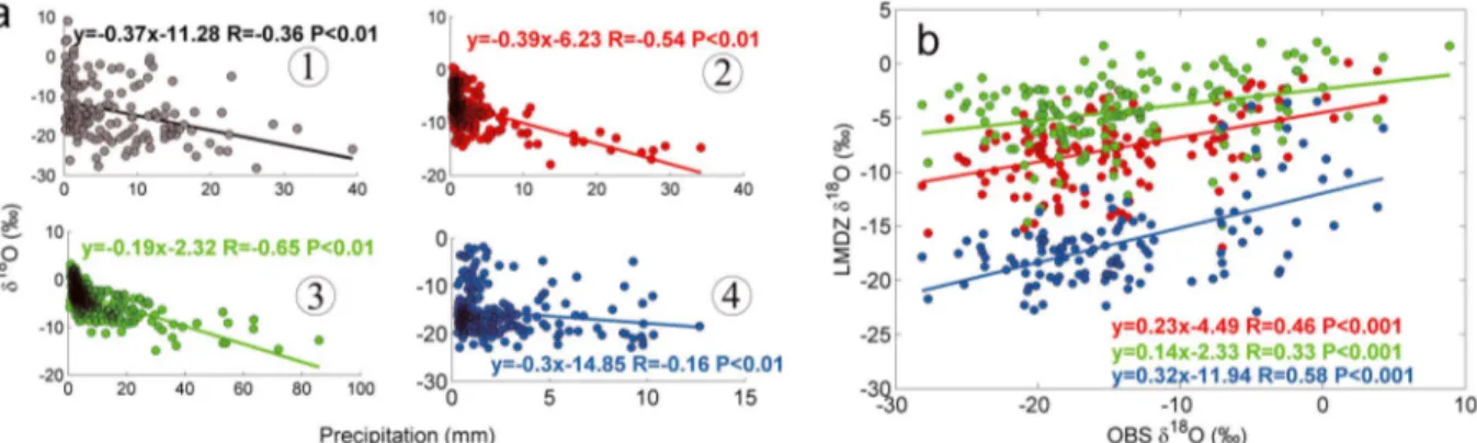
All versions of LMDZiso reasonably represent the relationship between precipitation amount and𝛿18O
p
(Figure 1a). At the daily scale, the Pearson correlation coefficients between the observed and simulated𝛿18O
p
are, respectively, 0.46 for LMDZiso Standard, 0.33 for LMDZiso NP, and 0.58 for LMDZiso Zoom in Figure 1b. Note that LMDZiso Zoom, with the highest horizontal resolution, can reasonably reproduce both the patterns and absolute values of𝛿18O
pin Lhasa. The weighted average JJAS𝛿18Opis −16.54‰ ±7.31‰ in the
observa-tions and −16.35‰ ±4.70‰ in LMDZiso Zoom. By contrast, LMDZiso Standard and NP produce much higher
𝛿18O
pvalues (−10.51‰ ± 3.43‰ and −6.62‰ ± 3.20‰ respectively), which may be due to the coarse
rep-resentation of the topography. For the simulation of precipitation, LMDZiso Standard reasonably reproduces the mean JJAS precipitation amount (400 mm ± 94 mm, against 360 mm ± 108 mm in the observations). By contrast, LMDZiso Zoom underestimates the precipitation amount at Lhasa (only 200 mm ± 99 mm) while LMDZiso NP overestimates observation(1000 mm ± 460 mm). The large standard deviation of precipitation in LMDZiso NP results from the large precipitation (1500 mm) in 2007 compared with precipitation in 2005 (770 mm) and in 2006 (750 mm).
Figure 1. The regressions of𝛿18Opwith daily precipitation amount (a) in JJAS from 2005 to 2007. The numbers 1, 2, 3, 4 represent the observation(black), LMDZiso Standard (red), NP version (green) and Zoom (blue) and (b) the comparison of𝛿18O
pat Lhasa between observation and simulations.
For visibility and simplicity, sometimes only the results for the standard version are shown, but we discuss whenever the three versions give different results. Figure 2 compares the observed and simulated atmo-spheric water vapor amount and𝛿Dvin LMDZiso. Compared with TES data, LMDZiso Standard can reasonably
reproduce the q-𝛿Dvdiagram, daily𝛿Dv, and q variability at 500 hPa (Figures 2a–2c). The comparison with
GOSAT data set (Figures 2d–2f ) also confirms LMDZiso’s ability for capturing isotopologue variability. The correlation coefficients between GOSAT observations and simulations are 0.65 (precipitable water) and 0.41 (𝛿Dv), respectively. Table 1 summarizes the comparison between the three LMDZiso versions and satellite
data. We note that none of the LMDZiso version perform unequivocally better than another and that there is no relationship between the model skills for local precipitation amount and for the isotopologue compo-sition of vapor and precipitation. Overall, the best performance is, for both averages and variability, obtained using Zoom version, consistent with previous studies [Gao et al., 2011; Yao et al., 2013], though it does not reasonably reproduce the isotopologue content retrieved from GOSAT.
Figure 2. (a–c) Comparison ofqand𝛿Dvproperties between the LMDZiso Standard simulation and the TES observa-tions at 500 hPa at Lhasa, for all months from 2005 to 2007: Figure 2a showsq −𝛿Dvdiagram retrieved from TES and simulated by LMDZiso, Figure 2b shows𝛿Dv, and Figure 2c showsqsimulated by LMDZiso as a function of the corre-sponding values retrieved from TES. (d–f ) Same as Figures 2a–2c but comparing the precipitable water and total column 𝛿Dvbetween the LMDZiso Standard simulation and the GOSAT observations. LMDZiso outputs were collocated with the TES or GOSAT data sets and applied the corresponding averaging kernels.
Table 1. Mean𝛿Dvandq, and Corresponding Standard Deviation at 500 hPa (TES/LMDZiso) or Integrated Over the Total Column (GOSAT/LMDZiso) Over Lhasa in JJASa
Statistics Observation Standard NP Zoom Mean𝛿Dv −242 ‰ −194 ‰ −185 ‰ −243 ‰ SD𝛿Dv 57 ‰ 41 ‰ 42 ‰ 45 ‰ TES r 1.0 0.61 0.44 0.67 Meanq 2.9 g/kg 3.3 g/kg 3.9 g/kg 3.7 g/kg SDq 1.2 g/kg 0.96 g/kg 0.76 g/kg 0.68 g/kg r 1.0 0.63 0.52 0.51 Mean𝛿Dv −165 ‰ −209 ‰ −177 ‰ −349 ‰ SD𝛿Dv 34 ‰ 36 ‰ 38 ‰ 45 ‰ GOSAT r 1.0 0.41 0.40 0.31 Meanq 9.8 g/kg 9.6 g/kg 13.4 g/kg 13.1 g/kg SDq 3.6 g/kg 2.1 g/kg 1.8 g/kg 1.3 g/kg r 1.0 0.65 0.46 0.21 Mean𝛿18O −16.54 ‰ −10.51 ‰ −6.62 ‰ −16.35 ‰ In situ SD𝛿18O 7.31 ‰ 3.43 ‰ 3.20 ‰ 4.70 ‰ r 1.0 0.46 0.33 0.58 aMean𝛿18O
pand corresponding standard deviation at Lhasa(Observation/ LMDZiso). The Standard, NP, Zoom represent the different versions of LMDZiso. We report the Pearson’s correlation coefficient between observations and LMDZiso.
LMDZiso produced a similar strength of correlation between𝛿Dvand𝛿18O
p, with correlation coefficients of
0.47 (Figure 3b) for LMDZiso Standard, 0.46 (p< 0.01)for LMDZiso NP and 0.56 (p < 0.01) for LMDZiso Zoom (figure not shown).
To summarize, this model-data comparison shows that LMDZiso is able to capture a significant fraction of the observed intraseasonal variability for both𝛿18O
pand𝛿Dvat Lhasa. In the following sections, we therefore use
LMDZiso to better understand the drivers of this isotopologue variability.
3.3. Link Between𝜹18O
pand𝜹Dvat Lhasa
To assess whether satellite𝛿Dvare suitable for investigating the controls of𝛿18Opat Lhasa, we show the
rela-tionship between𝛿Dvand𝛿18Opin Figure 3. The correlation coefficient between daily𝛿18Opobserved at Lhasa
and local TES𝛿Dvat 500 hPa is 0.43 (p < 0.01). This correlation can be explained by two factors. First, 𝛿Dp
and𝛿Dvare tightly correlated. Second,𝛿18Opis significantly and positively correlated with𝛿Dp. In LMDZiso
outputs, the correlation coefficient between daily summer variations of𝛿18O
p and𝛿Dp at Lhasa is 0.99.
Figure 3. The relationship between𝛿18O
pand𝛿Dvat Lhasa. (a)Observed𝛿18Opand𝛿Dvin TES at 500 hPa at Lhasa. (b) Same as Figure 3a but simulated by LMDZiso Standard.
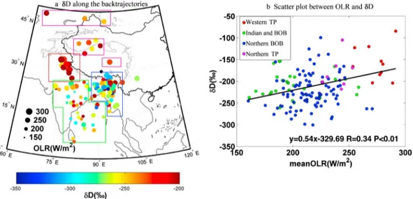
Figure 4. (a) Locations of air masses after 5 days along back trajectories from Lhasa. Back trajectories were launched for
days when TES data were available over Lhasa in JJAS from 2005 to 2007. The circle color represents the𝛿Dvat 500 hPa at Lhasa retrieved from TES, and the circle size represents the mean OLR along the back trajectories. (b)𝛿Dvat Lhasa as a function of mean OLR along the back trajectories. The linear regression is also shown.
This means that LMDZiso simulates limited variations in deuterium excess at the daily scale. It is consis-tent with daily observations at Lhasa [Tian et al., 2001b]. These findings indicate postcondensational do not significantly affect the variability of precipitation isotopologue composition.
Therefore, to understand the variability in the isotopologue composition of precipitation (𝛿18O
p), we now
focus on understanding the isotopologue composition of water vapor (𝛿Dv).
3.4. Relative Contribution of Moisture Source and of Convective Effects
Based on previous studies, the factors potentially controlling the𝛿18O
pof southern TP can be broadly
clas-sified into two effects: moisture source effects [Araguas-Araguas et al., 1998; Tian et al., 2001a; Tian, 2003; Yu
et al., 2008] and convective activity effects [Gao et al., 2013]. Here we explore the relative importance of these
two effects in JJAS combining𝛿Dvfrom TES, HYSPLIT back trajectories, and OLR data.
Figure 5. Spatial patterns of mean JJAS observed 𝛿Dv, from (a) TES (total column, 2005–2007) and (b) GOSAT
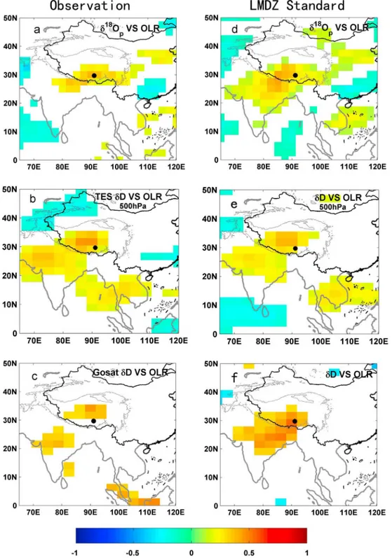
Figure 6. Daily correlation between the isotopologue composition (𝛿18Opor𝛿Dv) at Lhasa and OLR, in JJAS. (a)𝛿18Opat Lhasa. (b)𝛿Dvfrom TES at 500 hPa. (c) Column-integrated𝛿Dvfrom GOSAT. (d–f ) Same as Figures 6a–6c but for LMDZiso Standard. These correlations are straight correlations without removal of the seasonality and insignificant correlations are masked.
Figure 4a shows the locations of the 5 day back trajectories, average OLR values over the 5 day trajecto-ries, together with corresponding𝛿Dvat Lhasa.𝛿Dvis higher when trajectories come from the western (red
box) and northern (pink box) TP than when they come from the south (green and blue boxes). However, Figure 4b also shows that this apparent moisture source effect may reflects a convective effect. The vapor with low𝛿D values at Lhasa often transports over the regions with low OLR. This relationship holds for the
Figure 7. Daily correlations between𝛿Dvfrom TES at 500 hPa over Lhasa and OLR in surrounding areas at time leads of (a) 1, (b) 2, (c) 3, and (d) 4 days. These correlations are straight correlations without removal of the seasonality and insignificant correlations are masked.
main source regions and for the whole set of trajectories.𝛿Dvis higher over the south TP than over the north-ern TP (Figure 5). The low𝛿Dvvalues in the northern TP could be due to large-scale mixing with extratropical
water vapor sources with lower𝛿Dvvalues [Galewsky and Hurley, 2010; Noone, 2012]. The𝛿Dvspatial
distri-bution contrasts with the fact that water vapor coming from the southern TP contains lower𝛿Dvvalues at
Figure 8. Daily correlation between OLR in Northern India and specific humidity (q), as retrieved from TES (a) at 950 hPa and (b) at 500 hPa. (c, d) Same as Figures 8a and 8b but for𝛿Dvinstead ofq. These correlations are straight correlations without removal of the seasonality and insignificant correlations are masked.
Figure 9. Profiles ofq,𝛿Dv, and cloud cover both in NI and at Lhasa. (a, b) The profiles ofqon average (JJAS mean con-ditions) and anomalies during LOW-OLR-NI conditions, in NI and at Lhasa, respectively, retrieved from TES and simulated by LMDZiso. Anomalies are calculated with respect to the JJAS mean values. LOW-OLR-NI conditions are defined as days of strong convection over NI (based on OLR data, see text) at the time when air masses over NI. The time lag associated with the duration of the transport from NI to Lhasa, which corresponds to several days, is estimated based on the back trajectory calculation. For example, if an air mass takes 4 days to travel from NI to Lhasa, then LOW-OLR-NI conditions are determined using OLR data 4 days before. (c, d) As in Figures 9a and 9b but for𝛿Dv. (e, f ) As in Figures 9a and 9b but for CALIPSO cloud fraction from 2006 to 2007. In each subfigure, the left panel represents the mean condition and the right panel the difference between strong convection days and the mean condition.
Lhasa than the vapor coming from the northern TP. This confirms that what mainly controls the𝛿Dvat Lhasa at event scale in JJAS is not the𝛿Dvat the moisture source, but rather how the initial𝛿Dvis modified by convec-tive activity along the trajectories toward Lhasa. The moisture source has only an indirect effect, depending on whether air masses go through convective regions or not. We therefore conclude that the relationship between convective activity and𝛿Dvaccounts for most of the relationship between moisture source and𝛿Dv
in JJAS.
3.5. Relationship Between Convection and Isotopologue Composition
The previous section points out the importance of convective activity in controlling𝛿Dvat Lhasa. In this
section, we investigate in detail the importance of local and upstream convection effects.
Figure 6 shows the spatial correlations between the isotopologue composition of precipitation and water vapor at different pressure levels over Lhasa and the regional OLR, based on observations and on simula-tions performed with LMDZiso Standard. The effect of convective activity on the isotopologue composition is similar for both𝛿Dv(Figure 6) and𝛿18Op[Gao et al., 2013]. There is a significant positive correlation between
vapor (or precipitation) isotopologue abundance at Lhasa and OLR at the regional scale (NI and around Lhasa). The correlation pattern is consistent across different levels (500 hPa and total column) in all data sets (in situ precipitation, TES and GOSAT).
The temporal evolution of the relationship between𝛿Dvat 500 hPa at Lhasa and pre-Lhasa convective activity
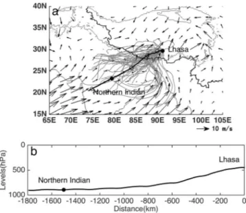
Figure 10. (a) JJAS mean wind vectors at 850 hPa from NCEP data set,
5 days back trajectories and mean back trajectory at Lhasa, (b) the altitude of mean trajectory at Lhasa. The circles represent locations for each of the 5 days along the trajectory.
NI increases from 0.30 (1 day ear-lier) to 0.35 (3 days earear-lier). Concur-rently, the correlation between 𝛿Dv
and OLR at Lhasa decreases. The pat-tern of relationships corresponds to the tracks of monsoon depressions that generate in the Bay of Ben-gal (BOB) (located at 10◦N–20◦Nand 80◦E–100◦E) and migrate northwest over NI [Rajamani and Sikdar, 1989]. Such consistencies indicate the poten-tial value of𝛿Dv in capturing signals
of Indian monsoon processes. Similar results are obtained with GOSAT data (not shown). Thus, water vapor 𝛿Dv
at Lhasa is more dependent on con-vection at the regional scale than at the local scale, consistent with previ-ous studies based on either precip-itation data or modeling [Gao et al., 2013; Schmidt et al., 2007; LeGrande
et al., 2009]. These findings suggest
that 𝛿Dv variations at Lhasa record changes in upstream convection, especially for those events that
occurred in NI.
LMDZiso Standard reasonably simulates these correlation patterns (Figures 6d–6f ) and their evolution through time (not shown). Similar results are obtained with LMDZiso Zoom and LMDZiso NP (not shown). This increases our confidence in using LMDZiso to study the link between NI convection and𝛿Dv.
4. How Does Deep Convective Activity Impact Vapor Isotopologue Composition?
Here we first investigate how deep convection affects𝛿Dv in NI, and then inquire how the follow-up
pro-cesses during transport affect𝛿Dv at Lhasa. We define the center of NI as the point located at 24◦N and
78.5◦E, because this is where we find the highest correlation, outside of the TP, between OLR and𝛿Dvin
Lhasa (Figure 6). Convective activity in this region is also a useful indicator of the strength of the Asian monsoon [Wang and Fan, 1999].
4.1. Influence of Convection in NI on Local Water Vapor𝜹Dv
Figure 8 shows the relationship between OLR in NI, specific humidity, and𝛿Dvat different pressure levels.
At 950 hPa, anticorrelation between OLR and q in NI (Figure 8a) arises because intense convection tends to occur when low-level q is high [Holloway and Neelin, 2010]. The positive correlation between OLR and𝛿Dv
at 950 hPa (Figure 8c) likely results from the impact of unsaturated downdrafts, which are enhanced with convective activity, reducing the low-level𝛿Dv[Risi et al., 2008a, 2010a]. Processes such as rain evaporation, rain-vapor exchanges, and moisture convergence can also contribute to reduced low-level𝛿Dv[Lawrence
et al., 2004; Worden et al., 2007; Risi et al., 2008a; Brown et al., 2008; Moore et al., 2014]. In the middle and upper
troposphere, low OLR is associated with moister air (Figure 8b), which could be due to the moistening effect of convective detrainment. In NI, there is no obvious local correlation between OLR and𝛿Dvin the middle and
upper troposphere (Figure 8d).
The positive correlation between OLR in NI and𝛿Dvin BOB may well arises from the northwestward
prop-agation of monsoon depressions [Rajamani and Sikdar, 1989; Goswami, 2005]. Along the track of monsoon depressions, the rainfall region shifts from BOB to NI. Strong convection over NI is also associated with stronger-than-normal convection over BOB. The daily correlation coefficient is 0.5 between OLR in NI and OLR above BOB in JJAS. In BOB, strong convective activity is related to low 𝛿Dv at middle and upper
atmospheric levels.
We conclude that convection in NI leads to decreases in low-level𝛿Dvlocally, and consequently affects𝛿Dv
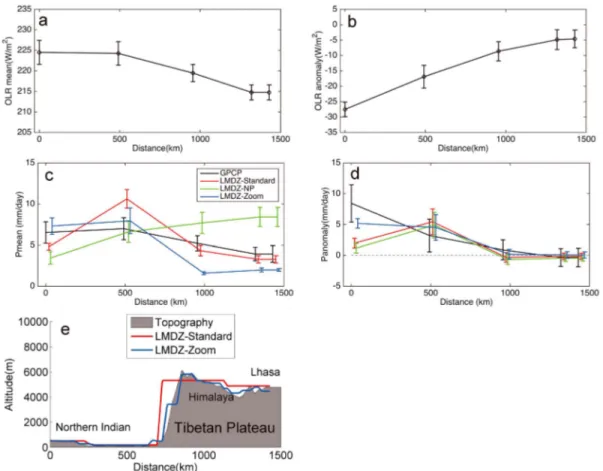
Figure 11. (a) Mean OLR along the back trajectory from Lhasa to Northern India and (b) OLR anomaly during
LOW-OLR-NI conditions, with respect to JJAS mean values. (c, d) Same as Figures 11a and 11b but for precipitation. (e) Topography along the back trajectory. The definition of LOW-OLR-NI conditions is the same as in Figure 9. The error bars represent plus or minus twice the standard error (𝜖) of the mean value. This standard error𝜖is calculated as the stan-dard deviation of the anomaly values divided by the square root of the number of anomaly values. Twice𝜖represent approximately the 95% confidence interval.
investigated in more detail. To do this, we examine days of strong convection in NI. When the NI OLR is lower than the JJAS mean OLR minus 40% of its standard deviation (28 W/m2), the day is defined as a strong con-vection day. Results are not qualitatively sensitive to the 40% threshold. Altogether, we identify 121 strong convection days in JJAS from 2005 to 2007. We calculate a composite of various variables for these specific strong convection days, and compare results with JJAS mean conditions.
As shown in Figure 9, strong convection days are associated with positive surface q and negative𝛿Dvanomaly.
TES data depict positive anomalies of𝛿Dvat middle and upper atmospheric levels (Figure 9c), where a positive
cloud anomaly is evidenced by CALIPSO data (Figure 9e). Increased cloud cover is associated with enhanced convective detrainment, which is associated with higher upper troposphere𝛿Dvvalues [Moyer et al., 1996; Risi et al., 2012; Worden et al., 2013; Jiang et al., 2013]. However, the positive middle-upper levels cloud anomaly
at Lhasa are inconsistent with negative𝛿Dvanomaly (Figures 9d and 9f ).
LMDZiso Standard and Zoom versions reasonably reproduce the mean vertical structure of q and𝛿Dv, while
LMDZiso NP overestimates humidity and deuterium levels above NI. Differences between LMDziso standard and zoom simulations are expected to arise from changes in topography. All LMDZiso versions reasonably capture the positive q anomaly associated with convection. However, all model versions fail to reproduce the positive𝛿Dvanomaly at middle-upper levels (Figure 9c, right). This discrepancy is due to misrepresentation of
the cloud vertical profile in LMDZiso. This is evidenced by comparing LMDZiso simulation to the CALIPSO data (Figure 9e). LMDZiso NP captures the positive cloud anomaly at upper atmospheric levels and thus reasonably reproduces the positive𝛿Dvanomaly at this level. However, it fails to reproduce the positive𝛿Dvanomaly
in the middle troposphere, which may be due to the misrepresentation of the cloud fraction at this level. In comparison, LMDZiso Standard fails to reproduce both cloud and𝛿Dvanomalies at middle and high levels.
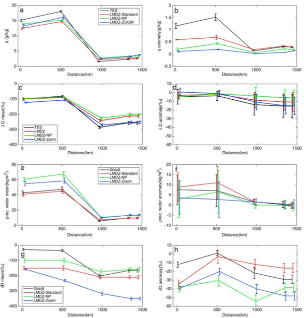
Figure 12. (a, c, e, and g) Mean observed and simulated values along the back trajectories. (b, d, f, and h) Anomalies
during LOW-OLR-NI conditions respect to JJAS mean values. Specific humidity (q) 100 hPa above the ground surface retrieved from TES (Figures 12a and 12b),𝛿Dv100 hPa above the ground surface retrieved from TES (Figures 12c and 12d), precipitable water retrieved from GOSAT (Figures 12e and 12f ), and column-integrated𝛿Dvretrieved from GOSAT (Figures 12g and 12h). Outputs simulated by LMDZ have been collocated and convolved by the appropriate averaging kernels. The definition of LOW-OLR-NI conditions is the same as in Figure 9. The error bars report plus or minus twice standard error of the mean value.
We investigate the vertical profile of𝛿Dv and cloud fraction at Lhasa 3 days after strong convection has occurred in NI. This lag was estimated from the correlation maps in Figure 7 and from the back trajectory analysis which is described in the next section.
4.2. Evolution of Water Vapor𝜹DvAlong Air Mass Trajectory
As discussed above, LMDZiso fails to reproduce the vertical𝛿Dvanomaly in NI. However, it does successfully
capture the𝛿Dvanomaly profile at Lhasa (Figure 9d). There is a positive relationship between𝛿Dvin TES at Lhasa and OLR (Figure 6b), yet a negative relationship between middle-upper levels𝛿Dvat NI and OLR (Figure 9c, right). We conclude that𝛿Dvanomalies at Lhasa are neither controlled by local convection and
clouds nor by NI cloud effects on the vertical𝛿Dvprofile in NI.
Back trajectories, launched from 1000 m AGL at Lhasa, were calculated for 5 days prior to launching in order to investigate the processes affecting the𝛿Dvprofile along the transport path. These back trajectories
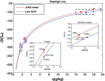
Figure 13. Rayleigh distillation theoretical line (solid line) and observed
in TES (open circle) in aq-𝛿Dvdiagram. The red line starts with JJAS mean conditions in Northern India (NI). The error bars report plus or minus twice standard error of the mean value. The blue line starts with LOW-OLR-NI conditions. The two subgraphs are centered on typical specific humidity values over Lhasa and NI. The definition of LOW-OLR-NI conditions is the same as in Figure 9.
can be grouped into two categories. First, trajectories from the northern and western parts of the TP are asso-ciated with low water vapor content [Feng and Zhou, 2012]. They corre-spond to only 12% of the total precip-itation amount at Lhasa in JJAS. The second class represents trajectories from the south, following the Indian monsoon, which transports consider-able vapor amounts [Tian et al., 2001a;
Feng and Zhou, 2012], responsible for
88% of the total precipitation amount at Lhasa in JJAS.
To investigate the link between 𝛿Dv
at Lhasa and convection in Northen India, we now focus on trajectories from the south. By averaging all tra-jectories, we produce a trajectory for a region from 75◦E to 84◦E and from 20◦N to 26◦N. Figure 10 shows these trajectories and the JJAS mean field from 2005 to 2007, consistent with the mean wind transport between NI and Lhasa. It takes about 4 days for the air traveling from NI to Lhasa. This is consistent with the maximum positive correlation between Lhasa𝛿Dvand NI OLR, obtained when OLR leads
𝛿Dvby 3 to 4 days. According to this average trajectory, the water vapor at Lhasa mainly travels from low
levels above NI (Figure 10b), consistent with previous studies [Feng and Zhou, 2012]. Surface air masses may well ascend the Himalaya due to mechanical and thermal forcing over the TP [Ye, 1981; Wu and Zhang, 1998;
Wu et al., 2007].
To understand the evolution of𝛿Dv, we need to understand the convection and condensation histories along
the trajectory. Figure 11 shows the mean and anomaly (i.e., when OLR is low in NI) of both OLR and precip-itation in JJAS along this trajectory. On average, OLR decreases from NI to the TP. Deeper into the TP, as air masses have already lost part of their moisture through rainout, precipitation amount decreases despite per-sistence of convective activity (Figures 11a and 11c). The OLR anomaly weakens along the trajectory from NI to Lhasa but remains negative. The small OLR anomaly near Lhasa is not significant. The precipitation anomaly identified from GPCP data decreases along the back trajectory, and it even becomes negative near Lhasa. The LMDZiso Zoom and LMDZiso Standard both reasonably capture the mean precipitation amount along the average trajectory (Figure 11), but LMDZiso NP underestimates north Indian precipitation and strongly over-estimates TP precipitation amount. It may thus misrepresent some processes controlling𝛿Dvin TP. LMDZiso
Zoom captures the positive TP precipitation anomaly associated with strong NI convection. LMDZiso NP and LMDZiso Standard exhibit a maximum precipitation anomaly value near the Himalaya foothills rather than in NI, where the largest precipitation is observed.
Figure 12 presents q,𝛿Dv, and precipitable water along the trajectory, retrieved from satellite, and simulated
by LMDZiso. Because the back trajectories follow the topography, we plot q and𝛿Dvat 100 hPa above the ground surface (Figures 12a and 12c). Since about 60% of the column-integrated water vapor is in the first 200 hPa above ground level regardless the topography, precipitable water, and total column𝛿Dvalong
trajec-tory (Figures 12e and 12g) can be compared to q and𝛿Dvat 100 hPa above the ground surface. On average,
the evolution of precipitable water and total column𝛿Dvfollows to first order the topography (Figure 12a, 12c, 12e, and 12g). The uplift to high-altitude results in decreased q and lower𝛿Dv.
The large positive q anomaly retrieved from TES during strong convection over the Himalaya foothills (Figure 12d) indicates that convection efficiently moistens air masses in this region. As already dis-cussed, strong convection activities decrease the low-level𝛿Dvin NI though there are large measurement
Figure 14. Contributions to the isotopologue budget at four locations (NI, Foothills, Himalaya, and Lhasa) along
the back trajectory, as computed by LMDZiso Standard. We show both JJAS mean values and anomalies during LOW-OLR-NI conditions with respect to JJAS mean values. The definition of LOW-OLR-NI conditions is the same as in Figure 9. The temporal derivative of𝛿Dvis decomposed into the effect of convection (cyan), large-scale advection (red), large-scale condensation (green), and surface evaporation and boundary layer mixing (dark blue). See text for more detail. (a) Vertical distribution of contributions to the isotopologue budget and (b) anomalies during LOW-OLR-NI conditions. (C) Contribution to the isotopologue budget at 100 hPa above ground surface and (d) anomalies during LOW-OLR-NI conditions.
uncertainties (Figure 12d). This initial anomaly is then amplified as air ascend over the Himalaya. GOSAT observations show consistent results.
All LMDZiso versions capture reasonably well the mean q, mean𝛿Dv and precipitable water along the
tra-jectory (Figure 12a, 12c, and 12e). During strong convection days above NI, all LMDZiso versions reasonably reproduce the low values of local surface𝛿Dv(except for the zoom model version in Figure 12d) and the ampli-fication of𝛿Dvanomalies over the Himalaya foothills, despite the difference in absolute values. Note that the
LMDZiso NP simulation of𝛿Dvis not superior despite the fact that this model version performs better for the
simulation of cloud cover (Figures 9e and 9f, section 4.2).
4.3. Amplification of𝜹DvAnomalies Over the Foothills by Rayleigh Processes
Here we aim to explain the mechanism amplifying the depletion of the vapor in HDO over the Himalaya foothills, following strong convection above NI. We hypothesize that this enhanced convection produces moister air masses, followed by enhanced condensation during the uplift on the Himalayan foothills. This more intense condensation is expected to decrease isotopologue composition. To test this hypothesis, we assume that the orographic condensation over the foothills can be modeled as a simple Rayleigh distillation. Figure 13 shows such Rayleigh distillation lines for JJAS mean conditions (red) and for days with strong con-vection in NI (blue), corresponding to the two types of NI initial conditions. At the start of the distillation line, the strong convection composite is characterized by water vapor with higher q and lower𝛿Dv(by −4‰ ). At
the end of the distillation line, at Lhasa, q is almost the same for the strong convection composite and for the JJAS mean conditions. This implies that more water vapor has been condensed along the transport path for the strong convection composite. This enhanced condensation leads to𝛿Dvat Lhasa being 9‰ lower for the composite than for JJAS mean conditions (Figure 13). This calculation supports our hypothesis that the𝛿Dv
Figure 15. Summary of our understanding of how convection in NI affects𝛿Dvover Lhasa along the back trajectory. The mean𝛿Dvvalues (a) for the mean state and (b) for LOW-OLR-NI conditions are indicated in italic. In parentheses, the mean𝛿Dvanomalies respect to mean state are also indicated. The definition of LOW-OLR-NI conditions is the same as in Figure 9. The green arrows represent large-scale vertical ascent. The yellow arrows represent the transport route from NI to Lhasa. The red arrows represent surface evaporation. The downward blue arrows represent unsaturated downdrafts.
anomaly amplification over the Himalaya foothills results from enhanced Rayleigh condensation processes. This is further supported by the large amount of precipitation over the Himalaya foothills.
Alternatively, the𝛿Dvover the Himalaya foothills may also decrease when mixing occurs with air masses from BOB, with low𝛿Dv. The BOB𝛿Dvis about 6‰ lower for the days with strong convection in NI than JJAS mean conditions. Therefore, large-scale mixing [Galewsky and Hurley, 2010; Noone, 2012] could also play a role in the𝛿Dvanomaly amplification.
4.4. Detailed Analysis of the Influence of Convection, Large-Scale Condensation, and Water Vapor Transport in the LMDZ Model
We have previously shown that LMDZiso is able, despite some caveats, to capture many aspects of the obser-vations. We now use LMDZiso simulations to understand the mechanisms explaining low𝛿Dvat Lhasa. Only
the results from the standard version are shown in Figure 14; similar results were found for other versions. For this purpose, we analyze the𝛿Dv change in water vapor isotopologue composition (i.e.,𝛿Dv change
with time) along the pathway.
In LMDZiso, water vapor is decomposed into four contributions: (1) advection by the large-scale dynamics (dyn); (2) large-scale condensation (lsc) which include the effect of in situ condensation in stratiform and oro-graphic clouds, and of the partial reevaporation of the precipitation; (3) convection (con) which includes the effects of unsaturated downdrafts, compensating subsidence, convective precipitation reevaporation and convective detrainment; and (4) surface evaporation and boundary layer mixing (vdf ).
Figure 14 shows the vertical distribution of the four contributions to the𝛿Dv from NI to Lhasa along the
back trajectory. The moisture budget has a very similar behavior to that of the𝛿Dvbudget: moistening
large-scale condensation (green) is always drying the vapor and lowering𝛿Dv, while advection (red) has
oppo-site effects. Near Lhasa, convection (cyan) dries low-level air and lessens low-level𝛿Dvvalues but moistens
middle to upper level air and increases middle to upper level𝛿Dvvalues by detrainment. Finally, surface
evaporation moistens low-level air and increases low-level𝛿Dvvalues.
According to LMDZ, the combination of enhanced large-scale condensation in the middle and upper tropo-sphere and enhanced convection near the surface (i.e., unsaturated downdrafts, left panels of Figure 14b) explains the coupling between strong convection and reduced𝛿Dvin NI. This feature is simulated both in NI and over the Himalaya foothills. LMDZ simulation confirms our understanding of how stronger convection in NI leads to reduced𝛿Dvin the low-level vapor in section 4.2. We also show change in the low-level vapor d𝛿Dv/dt (100 hPa above the ground surface) along the back trajectory (Figures 14c and 14d). For the average
JJAS conditions (Figure 14c), the unsaturated downdrafts and the large-scale condensation both contribute to the decrease in𝛿Dvalong the route to Lhasa. By contrast, both surface evaporation and advection increase 𝛿Dvalong the pathway. Figure 15 summarizes our understanding of the processes controlling the
intrasea-sonal variability of𝛿Dvat Lhasa.𝛿Dvvalues are more negative due to stronger unsaturated downdrafts over
NI on days of strong convection. These values are further decreased by more large-scale condensation over the Himalaya foothills before the air masses are transported to Lhasa.
5. Conclusion
This study aims at investigating the processes controlling the day-to-day summer variability of isotopologue composition observed in the southern TP. At Lhasa, observed𝛿18O
pand𝛿Dvare lowest in July and August
when moisture arrives at the site from Northern India. LMDZiso captures many features of the observations and can thus be used as a powerful tool to understand processes controlling the intraseasonal variability of TP vapor and precipitation isotopologue composition.
Paleorecords of𝛿18O
pare archived directly or indirectly in tree rings, speleothems, lake sediments, and glacier
ice. Our study has disentangled the processes at play for intraseasonal variations. However, in order to under-stand the paleoclimatic information preserved in natural archives from the southern TP, it is necessary to assess whether the underlying mechanisms responsible for the intraseasonal scale also explain the variability of the isotopologue signal at longer time scales, such as interannual, decadal, and also orbitally driven variations. Expanding this study to other regions of Tibet is also important, as ice core records from different regions of the southern TP reflect different control processes [Pang et al., 2014]. Intercomparing isotopic GCMs would allow us to investigate shortcomings in the model physics and to improve model’s capability for simulating the Southern TP isotopologue variability.
References
Aggarwal, P. K., K. Fröhlich, K. M. Kulkarni, and L. L. Gourcy (2004), Stable isotope evidence for moisture sources in the Asian summer monsoon under present and past climate regimes, Geophys. Res. Lett., 31, L08203, doi:10.1029/2004GL019911.
Araguas-Araguas, L., K. Froehlich, and K. Rozanski (1998), Stable isotope composition of precipitation over southeast Asia, J. Geophys. Res., 103(D22), 28,721–28,742, doi:10.1029/98JD02582.
Bao, Q., L. Pengfei, Z. Tianjun, and L. Yimin (2013), The flexible global ocean-atmosphere-land system model, spectral version 2: FGOALS-s2, Adv. Atmos. Sci., 30(3), 561–576, doi:10.1007/s00376-012-2113-9.
Bodas-Salcedo, A., et al. (2011), COSP: Satellite simulation software for model assessment, Bull. Am. Meteorol. Soc., 92 (8), 1023–1043, doi:10.1175/2011bams2856.1.
Brown, D., J. Worden, and D. Noone (2008), Comparison of atmospheric hydrology over convective continental regions using water vapor isotope measurements from space, J. Geophys. Res., 113, D15124, doi:10.1029/2007JD009676.
Chepfer, H., S. Bony, D. Winker, M. Chiriaco, J.-L. Dufresne, and G. Sèze (2008), Use of CALIPSO lidar observations to evaluate the cloudiness simulated by a climate model, Geophys. Res. Lett., 35, L15704, doi:10.1029/2008GL034207.
Chepfer, H., S. Bony, D. Winker, G. Cesana, J. L. Dufresne, P. Minnis, C. J. Stubenrauch, and S. Zeng (2010), The GCM-Oriented CALIPSO Cloud Product (CALIPSO-GOCCP), J. Geophys. Res., 115, D00H16, doi:10.1029/2009JD012251.
Coindreau, O., F. Hourdin, M. Haeffelin, A. Mathieu, and C. Rio (2007), Assessment of physical parameterizations using a global climate model with stretchable grid and nudging, Mon. Weather Rev., 135(4), 1474–1489, doi:10.1175/mwr3338.1.
Dansgaard, W., S. J. Johnsen, J. Møller, and C. C. Langway Jr. (1969), One thousand centuries of climatic record from Camp Century on the Greenland ice sheet, Science, 166(3903), 377–380, doi:10.1126/science.166.3903.377.
Draxler, R. R. (1998), An overview of the HYSPLIT4 modelling system for trajectories, dispersion, and deposition, Bur. Meteorol. Res. Centre, 47, 295–308.
Fabien, M., S. Dieter, M. Thomas, C. Emily, C. Julia, and F. Roman (2014), Precipitation seasonality and variability over the Tibetan Plateau as resolved by the high Asia reanalysis, J. Clim., 27, 1901–1927, doi:10.1175/JCLI-D-13-00282.1.
Feng, L., and T. Zhou (2012), Water vapor transport for summer precipitation over the Tibetan Plateau: Multidata set analysis, J. Geophys. Res., 117, D20114, doi:10.1029/2011JD017012.
Frankenberg, C., et al. (2009), Dynamic processes governing lower-troposphericHDO∕H2Oratios as observed from space and ground, Science, 325(5946), 1374–1377, doi:10.1126/science.1173791.
Acknowledgments
This work is supported by CAS Strategic Priority Research Program(B)-Interactions among Mul-tiple Geo-spheres on Tibetan Plateau and their Resource-Environment Effects (grant XDB03030100), by the National Natural Science Foundation of China (grants 41471053 and 41190080), and by the China-France Caiyuanpei Program. This work was finished in Lab-oratoire de Météorologie Dynamique, Institut Pierre Simon Laplace, CNRS, Paris, France. LMDZ simulations were performed on the supercomputer of the IDRIS computing center. Part of this research was carried out at the Jet Propulsion Laboratory, California Institute of Technology, under a con-tract with the National Aeronautics and Space Administration. C.-T Lai was supported by the U.S. National Science Foundation, Division of Atmospheric and Geo- space Sciences under Grant AGS-0956425. We thank Laurent Li and Pang Hongxi for their constructive comments. We also thank the staffs from Tibet observation stations for collecting the samples and staffs for measuring the samples, and all those who contributed to the field work. Part of in situ𝛿18Opdata are from Third Pole Environment Database (http://en. tpedatabase.cn/). The back trajectories and the OLR (Outgoing Longwave Radiation) are computed using National Centers for Environmental Prediction (NCEP) reanalysis data. LMDZiso data can be acquired by contacting Camille Risi (Camille.Risi@lmd.jussieu.fr). TES and GOSAT satellite data can also be acquired by contacting John Worden(john.r.worden@jpl.nasa.gov). CALIPSO data can also be acquired by contacting Gregory Cesana (gregory.cesana@lmd.polytechnique.fr). In situ𝛿18Opdata can also be acquired by contacting Gao Jing (gaojing@itpcas.ac.cn).


![[PDF] HTML CSS ss and bootstrap PDF [Eng] | Cours Bootstrap](data:image/gif;base64,R0lGODlhAQABAIAAAP///wAAACH5BAEAAAAALAAAAAABAAEAAAICRAEAOw==)