Differentiable programming for image processing and deep learning in halide

Differentiable programming for image

processing and deep learning in halide

The MIT Faculty has made this article openly available.

Please share

how this access benefits you. Your story matters.

Citation

Li, Tzu-Mao et al. "Differentiable programming for image processing

and deep learning in halide." ACM Transactions on Graphics 37, 4

(August 2018): 139 © 2018 The Authors

As Published

http://dx.doi.org/10.1145/3197517.3201383

Publisher

Association for Computing Machinery (ACM)

Version

Author's final manuscript

Citable link

https://hdl.handle.net/1721.1/122623

Terms of Use

Creative Commons Attribution-Noncommercial-Share Alike

Image Processing and Deep Learning in Halide

TZU-MAO LI,

MICHAËL GHARBI,

ANDREW ADAMS,

FRÉDO DURAND,

JONATHAN RAGAN-KELLEY,

d_grid d_guide

d_prior

(a) Neural network operator: bilateral slicing blurry input blur kernel prior output output

burst of RAW inputs homographies

reconstruction gradient

prior bilateral grid

d_loss d_loss

(b) optimizing the parameters of a

forward image processing pipeline warping parameters of an inverse problem(c) optimizing the reconstruction and warp input guide map d_loss d_H d_R d_guide

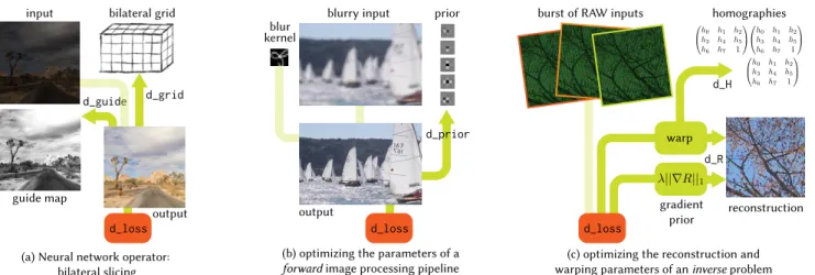
Fig. 1. Our system automatically derives and optimizes gradient code for general image processing pipelines, and yields state-of-the-art performance on both CPUs and GPUs. This enables a variety of imaging applications, from training novel neural network layers (a), to optimizing the parameters of traditional image processing pipelines (b), to solving inverse reconstruction problems (c). To support these applications, we extend the Halide language with features to automatically and efficiently compute gradients of arbitrary programs. We also introduce a new automatic performance optimization that can handle the specific computation patterns of gradient computation. Using our system, a user can easily write high-level image processing algorithms, and then automatically derive high-performance gradient code for CPUs, GPUs, and other architectures. Images from left to right are from MIT5k dataset [Bychkovsky et al. 2011], ImageNet [Deng et al. 2009], and deep demosaicking dataset [Gharbi et al. 2016], respectively.

Gradient-based optimization has enabled dramatic advances in computa-tional imaging through techniques like deep learning and nonlinear opti-mization. These methods require gradients not just of simple mathematical functions, but of general programs which encode complex transformations of images and graphical data. Unfortunately, practitioners have traditionally been limited to either hand-deriving gradients of complex computations, or composing programs from a limited set of coarse-grained operators in deep learning frameworks. At the same time, writing programs with the level of performance needed for imaging and deep learning is prohibitively difficult for most programmers.

We extend the image processing language Halide with general reverse-mode automatic differentiation (AD), and the ability to automatically opti-mize the implementation of gradient computations. This enables automatic computation of the gradients of arbitrary Halide programs, at high per-formance, with little programmer effort. A key challenge is to structure

Authors’ addresses: Tzu-Mao Li, MIT CSAIL, tzumao@mit.edu; Michaël Gharbi, MIT CSAIL, gharbi@mit.edu; Andrew Adams, Facebook AI Research, andrew.b.adams@ gmail.com; Frédo Durand, MIT CSAIL, fredo@mit.edu; Jonathan Ragan-Kelley, UC Berkeley & Google, jrk@berkeley.edu.

© 2018 Copyright held by the owner/author(s).

This is the author’s version of the work. It is posted here for your personal use. Not for redistribution. The definitive Version of Record was published in ACM Transactions on Graphics, https://doi.org/10.1145/3197517.3201383.

the gradient code to retain parallelism. We define a simple algorithm to automatically schedule these pipelines, and show how Halide’s existing scheduling primitives can express and extend the key AD optimization of “checkpointing.”

Using this new tool, we show how to easily define new neural network layers which automatically compile to high-performance GPU implemen-tations, and how to solve nonlinear inverse problems from computational imaging. Finally, we show how differentiable programming enables dra-matically improving the quality of even traditional, feed-forward image processing algorithms, blurring the distinction between classical and deep methods.

CCS Concepts: • Computing methodologies → Graphics systems and interfaces; Machine learning; Image processing;

Additional Key Words and Phrases: image processing, deep learning, auto-matic differentiation

ACM Reference Format:

Tzu-Mao Li, Michaël Gharbi, Andrew Adams, Frédo Durand, and Jonathan Ragan-Kelley. 2018. Differentiable Programming for Image Processing and Deep Learning in Halide. ACM Trans. Graph. 37, 4, Article 139 (August 2018), 13 pages. https://doi.org/10.1145/3197517.3201383

1 INTRODUCTION

Optimization and end-to-end learning are driving rapid progress in graphics and imaging, by viewing either the output image or large sets of pipeline parameters as unknowns, e.g. [Barron and Poole 2016; Gharbi et al. 2017; Heide et al. 2014; Jaderberg et al. 2015]. Key to this progress is the surprising power of gradient-based optimiza-tion methods to find soluoptimiza-tions to nonlinear objectives over large sets of unknowns. Unfortunately, the computation of gradients remains a challenge in the general case, especially when performance is paramount such as for training neural networks or when solving for images via optimization. Practitioners have to either manually derive gradients or they are limited to the composition of building blocks offered by deep learning libraries. The result is often ineffi-cient, and when users decide to stray from existing operators, the implementation of fast GPU derivative code is a major undertaking. At first glance, modern machine learning frameworks like Py-Torch, TensorFlow or CNTK [Abadi et al. 2015; Paszke et al. 2017; Yu et al. 2014] seem like appealing environments for new gradient-based graphics algorithms. When limited to their walled-gardens of pre-made, coarse-grained operations, these frameworks provide high-performance kernel implementations and automatic differenti-ation (AD) through chains of operdifferenti-ations. As general programming languages, however, they are a poor fit for many imaging applica-tions. Building new algorithms requires contorting a problem into complex and tangled compositions of existing building blocks. Even when done successfully, the resulting implementation is often both slow and memory-inefficient, saving and reloading entire arrays of intermediate results between each step, causing costly cache misses.

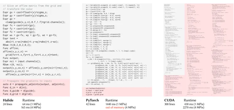
Consider the following example. A recent neural network-based image processing approximation algorithm was built around a new “bilateral slicing” layer based on the bilateral grid [Chen et al. 2007; Gharbi et al. 2017]. At the time it was published, neither PyTorch nor TensorFlow was even capable of practically expressing this computation.1As a result, the authors had to define an entirely new operator, written by hand in about 100 lines of CUDA for the forward pass and 200 lines more for its manually-derived gradient (Fig. 2, right). This was a sizeable programming task which took significant time and expertise. While new operations—added in just the last six months before the submission of this paper—now make it possible to implement this operation in 42 lines of PyTorch, this yields less than 1/3rd the performance on small inputs and runs out of memory on realistically-sized images (Fig. 2, middle). The challenge of efficiently deriving and computing gradients for custom nodes remains a serious obstacle to deep learning.

This pattern is ubiquitous. New custom nodes require major effort to implement correctly and efficiently, making it hard to experiment. Similarly, general image processing pipelines often do not map well to deep learning toolboxes. As a result, most researchers limit them-selves to consider only operations which are already well-supported by existing frameworks, while NVIDIA and the framework develop-ers must constantly expand the set of native operations. (There are currently at least 12 different kinds of convolution operator, alone, in TensorFlow.) The only alternative is to invest orders of magnitude 1_{Technically, TensorFlow graphs are Turing-complete, thanks to their inclusion of a} while loop node. However, implementing the algorithm at this level would be both incredibly complex and run at least thousands of times slower.

#include <THC/THC.h> #include <iostream> #include "math.h" extern THCState *state; __device__ float diff_abs(float x) { float eps = 1e-8; return sqrt(x*x+eps); } __device__ float d_diff_abs(float x) { float eps = 1e-8; return x/sqrt(x*x+eps); } __device__ float weight_z(float x) { float abx = diff_abs(x); return max(1.0f-abx, 0.0f); } __device__ float d_weight_z(float x) { float abx = diff_abs(x); if(abx > 1.0f) { return 0.0f; // return abx; } else { return d_diff_abs(x); } } __global__ void BilateralSliceApplyKernel( int64_t nthreads, const float* grid, const float* guide, const float* input, const int bs, const int h, const int w, const int gh, const int gw, const int gd, const int input_chans, const int output_chans, float* out) { // - Samples centered at 0.5. // - Repeating boundary conditions int grid_chans = (input_chans+1)*output_chans; int coeff_stride = input_chans+1; const int64_t idx = blockIdx.x*blockDim.x + threadIdx.x; if(idx < nthreads) { int x = idx % w; int y = (idx / w) % h; int out_c = (idx / (w*h)) % output_chans; int b = (idx / (output_chans*w*h)); float gx = (x+0.5f)*gw/(1.0f*w); float gy = (y+0.5f)*gh/(1.0f*h); float gz = guide[x + w*(y + h*b)]*gd; int fx = static_cast<int>(floor(gx-0.5f)); int fy = static_cast<int>(floor(gy-0.5f)); int fz = static_cast<int>(floor(gz-0.5f)); // Grid strides int sx = 1; int sy = gw; int sz = gw*gh; int sc = gw*gh*gd; int sb = grid_chans*gd*gw*gh; float value = 0.0f; for (int in_c = 0; in_c < coeff_stride; ++in_c) { float coeff_sample = 0.0f; for (int xx = fx; xx < fx+2; ++xx) { int x_ = max(min(xx, gw-1), 0); float wx = max(1.0f-abs(xx+0.5-gx), 0.0f); for (int yy = fy; yy < fy+2; ++yy) { int y_ = max(min(yy, gh-1), 0); float wy = max(1.0f-abs(yy+0.5-gy), 0.0f); for (int zz = fz; zz < fz+2; ++zz) { int z_ = max(min(zz, gd-1), 0); float wz = weight_z(zz+0.5-gz); int grid_idx = sc*(coeff_stride*out_c + in_c) + sz*z_ + sx*x_ + sy*y_ + sb*b; coeff_sample += grid[grid_idx]*wx*wy*wz; } } } // Grid trilinear interpolation if(in_c < input_chans) { int input_idx = x + w*(y + input_chans*(in_c + h*b)); value += coeff_sample*input[input_idx]; } else { // Offset term value += coeff_sample; } } out[idx] = value; } } __global__ void BilateralSliceApplyGridGradKernel( int64_t nthreads, const float* grid, const float* guide, const float* input, const float* d_output, const int bs, const int h, const int w, const int gh, const int gw, const int gd, const int input_chans, const int output_chans, float* out) { int grid_chans = (input_chans+1)*output_chans; int coeff_stride = input_chans+1; const int64_t idx = blockIdx.x*blockDim.x + threadIdx.x; if(idx < nthreads) { int gx = idx % gw; int gy = (idx / gw) % gh; int gz = (idx / (gh*gw)) % gd; int c = (idx / (gd*gh*gw)) % grid_chans; int b = (idx / (grid_chans*gd*gw*gh)); float scale_w = w*1.0/gw; float scale_h = h*1.0/gh; int left_x = static_cast<int>(floor(scale_w*(gx+0.5-1))); int right_x = static_cast<int>(ceil(scale_w*(gx+0.5+1))); int left_y = static_cast<int>(floor(scale_h*(gy+0.5-1))); int right_y = static_cast<int>(ceil(scale_h*(gy+0.5+1))); // Strides in the output int sx = 1;

int sy = w; int sc = h*w; int sb = output_chans*w*h; // Strides in the input int isx = 1; int isy = w; int isc = h*w; int isb = output_chans*w*h; int out_c = c / coeff_stride; int in_c = c % coeff_stride; float value = 0.0f; for (int x = left_x; x < right_x; ++x) { int x_ = x; // mirror boundary if (x_ < 0) x_ = -x_-1; if (x_ >= w) x_ = 2*w-1-x_; float gx2 = (x+0.5f)/scale_w; float wx = max(1.0f-abs(gx+0.5-gx2), 0.0f); for (int y = left_y; y < right_y; ++y) { int y_ = y; // mirror boundary if (y_ < 0) y_ = -y_-1; if (y_ >= h) y_ = 2*h-1-y_; float gy2 = (y+0.5f)/scale_h; float wy = max(1.0f-abs(gy+0.5-gy2), 0.0f); int guide_idx = x_ + w*y_ + h*w*b; float gz2 = guide[guide_idx]*gd; float wz = weight_z(gz+0.5f-gz2); if ((gz==0 && gz2<0.5f) || (gz==gd-1 && gz2>gd-0.5f)) { wz = 1.0f; } int back_idx = sc*out_c + sx*x_ + sy*y_ + sb*b; if (in_c < input_chans) { int input_idx = isc*in_c + isx*x_ + isy*y_ + isb*b; value += wz*wx*wy*d_output[back_idx]*input[input_idx]; } else { // offset term value += wz*wx*wy*d_output[back_idx]; } } } out[idx] = value; } } __global__ void BilateralSliceApplyGuideGradKernel( int64_t nthreads, const float* grid, const float* guide, const float* input, const float* d_output, const int bs, const int h, const int w, const int gh, const int gw, const int gd, const int input_chans, const int output_chans, float* out) { int grid_chans = (input_chans+1)*output_chans; int coeff_stride = input_chans+1; const int64_t idx = blockIdx.x*blockDim.x + threadIdx.x; if(idx < nthreads) { int x = idx % w; int y = (idx / w) % h; int b = (idx / (w*h)); float gx = (x+0.5f)*gw/(1.0f*w); float gy = (y+0.5f)*gh/(1.0f*h); float gz = guide[x + w*(y + h*b)]*gd; int fx = static_cast<int>(floor(gx-0.5f)); int fy = static_cast<int>(floor(gy-0.5f)); int fz = static_cast<int>(floor(gz-0.5f)); // Grid stride int sx = 1; int sy = gw; int sz = gw*gh; int sc = gw*gh*gd; int sb = grid_chans*gd*gw*gh; float out_sum = 0.0f; for (int out_c = 0; out_c < output_chans; ++out_c) { float in_sum = 0.0f; for (int in_c = 0; in_c < coeff_stride; ++in_c) { float grid_sum = 0.0f; for (int xx = fx; xx < fx+2; ++xx) { int x_ = max(min(xx, gw-1), 0); float wx = max(1.0f-abs(xx+0.5-gx), 0.0f); for (int yy = fy; yy < fy+2; ++yy) { int y_ = max(min(yy, gh-1), 0); float wy = max(1.0f-abs(yy+0.5-gy), 0.0f); for (int zz = fz; zz < fz+2; ++zz) { int z_ = max(min(zz, gd-1), 0); float dwz = gd*d_weight_z(zz+0.5-gz); int grid_idx = sc*(coeff_stride*out_c + in_c) + sz*z_ + sx*x_ + sy*y_ + sb*b; grid_sum += grid[grid_idx]*wx*wy*dwz; } // z } // y } // x, grid trilinear interp if(in_c < input_chans) { in_sum += grid_sum*input[input_chans*(x+w*(y+h*(in_c+input_chans*b)))]; } else { // offset term in_sum += grid_sum; } } // in_c

out_sum += in_sum*d_output[x + w*(y + h*(out_c + output_chans*b))]; } // out_c

out[idx] = out_sum; } }

__global__ void BilateralSliceApplyInputGradKernel( int64_t nthreads, const float* grid, const float* guide, const float* input, const float* d_output, const int bs, const int h, const int w, const int gh, const int gw, const int gd, const int input_chans, const int output_chans, float* out) { int grid_chans = (input_chans+1)*output_chans; int coeff_stride = input_chans+1; const int64_t idx = blockIdx.x*blockDim.x + threadIdx.x; if(idx < nthreads) { int x = idx % w; int y = (idx / w) % h; int in_c = (idx / (w*h)) % input_chans; int b = (idx / (input_chans*w*h)); float gx = (x+0.5f)*gw/(1.0f*w); float gy = (y+0.5f)*gh/(1.0f*h); float gz = guide[x + w*(y + h*b)]*gd; int fx = static_cast<int>(floor(gx-0.5f)); int fy = static_cast<int>(floor(gy-0.5f)); int fz = static_cast<int>(floor(gz-0.5f)); // Grid stride int sx = 1; int sy = gw; int sz = gw*gh; int sc = gw*gh*gd; int sb = grid_chans*gd*gw*gh; float value = 0.0f; for (int out_c = 0; out_c < output_chans; ++out_c) { float chan_val = 0.0f; for (int xx = fx; xx < fx+2; ++xx) { int x_ = max(min(xx, gw-1), 0); float wx = max(1.0f-abs(xx+0.5-gx), 0.0f); for (int yy = fy; yy < fy+2; ++yy) { int y_ = max(min(yy, gh-1), 0); float wy = max(1.0f-abs(yy+0.5-gy), 0.0f); for (int zz = fz; zz < fz+2; ++zz) { int z_ = max(min(zz, gd-1), 0); float wz = weight_z(zz+0.5-gz); int grid_idx = sc*(coeff_stride*out_c + in_c) + sz*z_ + sx*x_ + sy*y_ + sb*b; chan_val += grid[grid_idx]*wx*wy*wz; } // z } // y } // x, grid trilinear interp value += chan_val*d_output[x + w*(y + h*(out_c + output_chans*b))]; } // out_c out[idx] = value; } } // -- KERNEL LAUNCHERS ---void BilateralSliceApplyKernelLauncher( int bs, int gh, int gw, int gd, int input_chans, int output_chans, int h, int w, const float* const grid, const float* const guide, const float* const input, float* const out) { int total_count = bs*h*w*output_chans; const int64_t block_sz = 512; const int64_t nblocks = (total_count + block_sz - 1) / block_sz; if (total_count > 0) { BilateralSliceApplyKernel<<< nblocks, block_sz, 0, THCState_getCurrentStream(state)>>>( total_count, grid, guide, input, bs, h, w, gh, gw, gd, input_chans, output_chans, out); THCudaCheck(cudaPeekAtLastError()); } } void BilateralSliceApplyGradKernelLauncher( int bs, int gh, int gw, int gd, int input_chans, int output_chans, int h, int w, const float* grid, const float* guide, const float* input, const float* d_output, float* d_grid, float* d_guide, float* d_input) {

int64_t coeff_chans = (input_chans+1)*output_chans; const int64_t block_sz = 512; int64_t grid_count = bs*gh*gw*gd*coeff_chans; if (grid_count > 0) { const int64_t nblocks = (grid_count + block_sz - 1) / block_sz; BilateralSliceApplyGridGradKernel<<< nblocks, block_sz, 0, THCState_getCurrentStream(state)>>>( grid_count, grid, guide, input, d_output, bs, h, w, gh, gw, gd, input_chans, output_chans, d_grid); } int64_t guide_count = bs*h*w; if (guide_count > 0) { const int64_t nblocks = (guide_count + block_sz - 1) / block_sz; BilateralSliceApplyGuideGradKernel<<< nblocks, block_sz, 0, THCState_getCurrentStream(state)>>>( guide_count, grid, guide, input, d_output, bs, h, w, gh, gw, gd, input_chans, output_chans, d_guide); } int64_t input_count = bs*h*w*input_chans; if (input_count > 0) { const int64_t nblocks = (input_count + block_sz - 1) / block_sz; BilateralSliceApplyInputGradKernel<<< nblocks, block_sz, 0, THCState_getCurrentStream(state)>>>( input_count, grid, guide, input, d_output, bs, h, w, gh, gw, gd, input_chans, output_chans, d_input); } } 308 lines CUDA 2270 ms (4 MPix)430 ms (1 MPix) Runtime

xx = Variable(th.arange(0, w).cuda().view(1, -1).repeat(h, 1)) yy = Variable(th.arange(0, h).cuda().view(-1, 1).repeat(1, w)) gx = ((xx+0.5)/w) * gw gy = ((yy+0.5)/h) * gh gz = th.clamp(guide, 0.0, 1.0)*gd fx = th.clamp(th.floor(gx - 0.5), min=0) fy = th.clamp(th.floor(gy - 0.5), min=0) fz = th.clamp(th.floor(gz - 0.5), min=0) wx = gx - 0.5 - fx wy = gy - 0.5 - fy wx = wx.unsqueeze(0).unsqueeze(0) wy = wy.unsqueeze(0).unsqueeze(0) wz = th.abs(gz-0.5 - fz) wz = wz.unsqueeze(1) fx = fx.long().unsqueeze(0).unsqueeze(0) fy = fy.long().unsqueeze(0).unsqueeze(0) fz = fz.long() cx = th.clamp(fx+1, max=gw-1); cy = th.clamp(fy+1, max=gh-1); cz = th.clamp(fz+1, max=gd-1) fz = fz.view(bs, 1, h, w) cz = cz.view(bs, 1, h, w)

batch_idx = th.arange(bs).view(bs, 1, 1, 1).long().cuda() out = []

co = c // (ci+1) for c_ in range(co):

c_idx = th.arange((ci+1)*c_, (ci+1)*(c_+1)).view(\ 1, ci+1, 1, 1).long().cuda()

a = grid[batch_idx, c_idx, fz, fy, fx]*(1-wx)*(1-wy)*(1-wz) + \ grid[batch_idx, c_idx, cz, fy, fx]*(1-wx)*(1-wy)*( wz) + \ grid[batch_idx, c_idx, fz, cy, fx]*(1-wx)*( wy)*(1-wz) + \ grid[batch_idx, c_idx, cz, cy, fx]*(1-wx)*( wy)*( wz) + \ grid[batch_idx, c_idx, fz, fy, cx]*( wx)*(1-wy)*(1-wz) + \ grid[batch_idx, c_idx, cz, fy, cx]*( wx)*(1-wy)*( wz) + \ grid[batch_idx, c_idx, fz, cy, cx]*( wx)*( wy)*(1-wz) + \ grid[batch_idx, c_idx, cz, cy, cx]*( wx)*( wy)*( wz) o = th.sum(a[:, :-1, ...]*input, 1) + a[:, -1, ...] out.append(o.unsqueeze(1)) out = th.cat(out, 1) out.backward(adjoints) d_input = input.grad d_grid = grid.grad d_guide = guide.grad PyTorch

42 lines Runtime1440 ms (1 MPix)

out of memory (4 MPix)

// Slice an affine matrix from the grid and // transform the color

Expr gx = cast<float>(x)/sigma_s; Expr gy = cast<float>(y)/sigma_s; Expr gz = clamp(guide(x,y,n),0.f,1.f)*grid.channels(); Expr fx = cast<int>(gx); Expr fy = cast<int>(gy); Expr fz = cast<int>(gz); Expr wx = gx-fx, wy = gy-fy, wz = gz-fz; Expr tent = abs(rt.x-wx)*abs(rt.y-wy)*abs(rt.z-wz); RDom rt(0,2,0,2,0,2); Func affine; affine(x,y,c,n) += grid(fx+rt.x,fy+rt.y,fz+rt.z,c,n)*tent; Func output;

Expr nci = input.channels(); RDom r(0, nci);

output(x,y,co,n) = affine(x,y,co*(nci+1)+nci,n); output(x,y,co,n) +=

affine(x,y,co*(nci+1)+r,n) * in(x,y,r,n); // Propagate the gradients to inputs auto d = propagate_adjoints(output, adjoints); Func d_in = d(in);

Func d_guide = d(guide); Func d_grid = d(grid);

Halide Runtime 24 lines 64 ms (1 MPix)

165 ms (4 MPix)

Fig. 2. Implementations of the forward and gradient computations of the bilateral slicing layer [Gharbi et al. 2017] in Halide, PyTorch, and CUDA. Using our automatic differentiation and scheduling extensions, the Halide implementation is clear, concise, and fast. The PyTorch implementation is modestly more complex, but runs 20× slower on a 1k × 1k input, fails to complete (out of memory on a 12GB NVIDIA Titan Xp) on a 2k × 2k input, and is only possible thanks to new operators added to PyTorch since the original publication. The CUDA implementation, developed by the original authors, is not only complex (an order of magnitude larger than either Halide or PyTorch), but is dominated by hand-derived gradient computations. It is faster than PyTorch and scales to larger inputs, but is still about 10× slower than the Halide version. Note: code size includes a few lines beyond the core logic shown for both Halide and PyTorch.

more effort in developing custom operations, hand-deriving, reim-plementing, and debugging gradient code for every change during the development of a new algorithm.

Recently, the Halide domain-specific language [Ragan-Kelley et al. 2012, 2013] has enabled the implementation of high-performance image-processing pipelines. It is an effective solution to implement-ing custom nodes and general image processimplement-ing pipelines, but it still requires the manual derivation of gradients. Furthermore, our experience shows that the computation pattern of derivatives dif-fers from that of forward code, which causes existing automatic performance optimizations in Halide to fail. Critically, the current built-in Halide autoscheduler does not support GPU schedules.

In this paper, we extend Halide with methods to automatically and efficiently compute the gradients of arbitrary Halide programs using reverse-mode automatic differentiation (Sec. 4). This transformation supports all existing features in the language.

Building atop Halide has several advantages. It provides a concise, natural language in which to express image processing computa-tions, and for which there is already a library of existing algorithms. The Halide compiler portably targets numerous processor and ac-celerator architectures, from mobile CPUs, to image processing DSPs, to data center GPUs, and supports compilation to very high-performance code. Finally, Halide’s existing language and schedul-ing constructs compose with reverse-mode AD to naturally express and generalize essential optimizations from the traditional AD liter-ature (Sec. 4.3). Key to making our compiler transformation work are a scatter-to-gather conversion algorithm which preserves par-allelism (Sec. 4.2.1), and a simple automatic scheduling algorithm specialized to the patterns that appear in generated gradient code (Sec. 4.4). Halide’s existing system of powerful dependence analyses is essential for both. In contrast to traditional Halide, automatic scheduling is critical given the complexity of the automatically-generated gradient code.

Using our new automatic gradient computation and automatic scheduler, we show how we can easily implement three recently-proposed neural network layers using code that is both faster and significantly simpler than the authors’ original custom nodes writ-ten in C++ and CUDA (Sec. 5.1). For example, the aforementioned bilateral slicing layer is expressed in 24 lines of Halide (Fig. 2, left), including just four lines to compute and extract its gradients, while compiling automatically to an implementation about 10× faster than the authors’ original handwritten CUDA, and 20× faster than a more limited version in PyTorch. We believe that this ease of implementa-tion and performance tuning will dramatically facilitate prototyping, by delivering both automatic gradients and high performance at the outset of experimentation, not after-the-fact once the usefulness of a node has been established, but as soon as experimentation begins. We also argue that this approach of gradient-based optimization through arbitrary programs is useful outside the traditional deep learning applications which have popularized it. Our vision is that any image-processing pipelines can benefit from an automatic tun-ing of internal parameters. Currently, this step is usually done by hand through user trial-and-error. The availability of automatic derivatives makes it possible to systematically optimize any inter-nal parameter of an image processing pipeline, given some output objectives. This is especially appealing when gradients are available

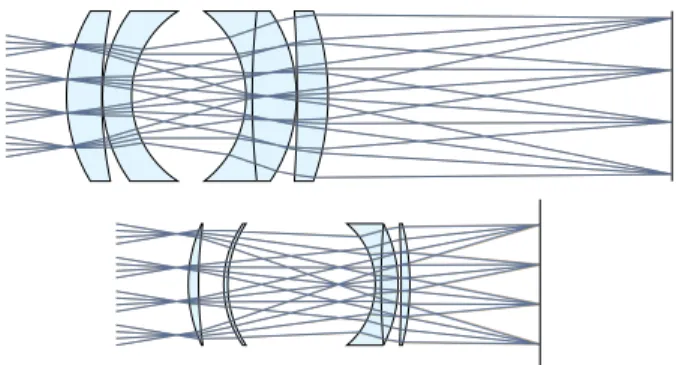
in the same language used for high-performance code deployment. We show how to significantly improve the performance of two tra-ditional image processing algorithms by automatically optimizing their key parameters and filters (Sec. 5.2). We also implement a novel joint burst demosaicking and superresolution algorithm by inverting a forward image formation model including warps by unknown homographies, solving for the image and homographies simultaneously (Sec. 5.3). Finally, we show the versatility of our ap-proach and implement a lens design optimization by differentiating an optical simulator (Sec. 5.4).

2 RELATED WORK

2.1 Automatic differentiation

Automatic differentiation is a collection of techniques to numerically evaluate the derivatives of a computer program [Griewank and Walther 2008]. Automatic differentiation is distinct from both finite differences and symbolic differentiation. It exploits the structure of the computation graph by recursively applying the chain rule, and it synthesizes a new program that computes the derivatives, instead of closed-form algebraic expressions. To compute the gradient of a scalar output, traversing the computation graph backwards from the output to propagate the adjoints to all the inputs gives the same time complexity as the original program (e.g. [Linnainmaa 1970; Werbos 1982]. Automatic differentiation has been rediscovered as “backpropagation” for neural networks [Rumelhart et al. 1986]).

Although the time complexity of the gradient computation matches that of the original program, the backward traversal can use signifi-cantly more memory than the forward pass. Traditional automatic differentiation systems trade off between memory and run time us-ing a checkpointus-ing strategy [Volin and Ostrovskii 1985]. Our system allows the user to explore the space of trade-offs using scheduling mechanisms provided by the Halide language (Sec. 4.3).

Many automatic differentiation frameworks have been developed for general programming languages [Bischof et al. 1992; Griewank et al. 1996; Hascoet and Pascual 2013; Hogan 2014; Wiltschko et al. 2017], but general programming languages can be cumbersome for image processing applications. Writing efficient image processing code requires enormous efforts to take parallelism, locality, and memory consumption/bandwidth into account [Ragan-Kelley et al. 2012]. These difficulties are compounded when we also want to compute derivatives. Other recent packages provide higher level, highly optimized differentiable building blocks for users to assemble their program [Abadi et al. 2015; Bergstra et al. 2010; Paszke et al. 2017; Yu et al. 2014]. These packages are efficient when the algorithm to be implemented can be conveniently expressed by combining these building blocks. But it is quite common for users to write their own custom operators in low-level C++ or CUDA to extend a package’s functionalities. This means that users have to write code for both the forward program and its gradients, and make sure they are correct, consistent and reasonably efficient. This can be tedious, error-prone and challenging to maintain. Using our approach, one can simply write the forward program. Our algorithm generates the derivatives and, thanks to Halide’s decoupling of algorithm and schedule and our automatic scheduler, provides convenient handles to easily produce efficient code.

2.2 Image processing languages

Our work builds on the Halide [Ragan-Kelley et al. 2012] image processing language, which we briefly introduce in Sec. 3.

The Opt language [Devito et al. 2017] focuses on nonlinear least squares problems. It provides language constructs to describe least squares cost and automatically generates solvers. It uses the D* algo-rithm [Guenter 2007] to generate derivatives. The ProxImaL [Heide et al. 2016] language, on the other hand, focuses on solving inverse problems using proximal gradient algorithms. The language pro-vides a set of functions and their corresponding proximal operators. It then generates Halide code for optimization. Our system can be used to generate the adjoints required by new ProxImaL operators. These languages focus on a specific set of solvers, namely nonlinear least squares and proximal methods, and provide high-level inter-faces to them. On the other hand, we deal with any problem that requires the gradient of a program. Our system can also be used to solve for unknowns other than images, such as optimizing the hyperparameters of an algorithm or jointly optimizing images and parameters. Sec. 5.3 demonstrates this with some examples.

Recently, there have been attempts to automatically speed-up image processing pipelines [Mullapudi et al. 2016, 2015; Yang et al. 2016]. We developed a new automatic scheduler in Halide with specialized mechanisms for parallel reductions [Suriana et al. 2017], which often occur in the derivatives of image processing code. Our system could further benefit from future developments in automatic code optimization.

2.3 Learning and optimizing with images

Gradient-based optimization is commonly used in image processing. It has been used for image restoration [Rudin et al. 1992], image registration [Zitova and Flusser 2003], optical flow estimation [Horn and Schunck 1981], stereo vision [Barron and Poole 2016], learn-ing image priors [Roth and Black 2005; Ulyanov et al. 2017] and solving complex inverse problems [Heide et al. 2014]. Our work alle-viates the need to manually derive the gradient in such applications, which enables faster experimentation. Deep learning has revital-ized an interest in building differentiable forward image processing pipelines whose parameters can be tuned by stochastic gradient descent. Successful instances include image restoration [Gharbi et al. 2016; Zhang et al. 2017], photographic enhancement [Xu et al. 2015], and applications such as colorization [Iizuka et al. 2016; Zhang et al. 2016], and style transfer [Gatys et al. 2016; Luan et al. 2017]. Some of these methods call for custom operators [Gharbi et al. 2017; Ilg et al. 2017; Jaderberg et al. 2015], typically not available in main-stream frameworks. For these custom operators, the forward and gradient operations are implemented manually. Our work provides a convenient way to explore new custom computations.

3 THE HALIDE PROGRAMMING LANGUAGE

Our system extends the Halide programming language. We will give a brief overview of the constructs in Halide that are relevant to our system. For more detail on Halide, see the original papers [Ragan-Kelley et al. 2012, 2013] and documentation.1

1_{http://halide-lang.org/}

Halide is a language designed to make it easy to write high-performance image- and array-processing code. The key idea in Halide is the separation of a program into the algorithm, which specifies what is computed, and the schedule, which dictates the order of computation and storage. The algorithm is expressed as a pure functional, feed-forward pipeline of arithmetic operations on multidimensional grids. The schedule addresses concerns such as tiling, vectorization, parallelization, mapping to a GPU, etc. The language guarantees that the output of a program depends only on the algorithm and not on the schedule. This frees the user from worrying about low-level optimizations while writing the high-level algorithm. They can then explore optimization strategies without unintentionally altering the output.

By adding automatic differentiation to Halide, we build on this philosophy. To create a differentiable pipeline, the user no longer needs to worry about the correctness and efficiency of the gradient code. With the sole specification of a forward algorithm, our system synthesizes the gradient algorithm. Optimization strategies can then be explored for both, either manually or with an auto-scheduler.

The following code shows an example Halide program that per-forms gamma correction on an image and computes theL2norm between the output and a target image:

Param<float> g;// Gamma parameter

Buffer<float> im, tgt;// 2−_{D input and target buffers}

Var x, y;// Integer variables for the pixel coordinates

Funcf;// Halide function declarations // Halide function definition

f(x, y) = pow(im(x, y), g);

// Reduction variables to loop over target's domain

RDomr(tgt);

Funcloss; // We compute the MSE loss between f and tgt loss() = 0.f; // Initialize the sum to 0

Exprdiff = f(r.x, r.y)−tgt(r.x, r.y); loss() += diff * diff; // Update definition

Halide is embedded in C++. Halide pipeline stages are called func-tions and represented in code by the C++ classFunc. Each Halide function is defined over an n-dimensional grid. The definition of a function comprises:

• an initial value that specifies a value for each grid point. • optional recursive updates that modify these values in-place. The function definitions are specified as Halide expressions (objects of typeExpr). Halide expressions are side-effect-free, including arith-metic, logical expressions, conditionals, and calls to other Halide functions, input buffers, or external code (such assinorexp).

Reduction operators, such as summation or general convolution, are implemented through recursive updates of a Halide function. The domain of a reduction is represented in code as anRDom, which implies a loop over that domain. All loops in Halide are implicit, whether over the domain of a function or a reduction.

Scheduling is expressed through methods exposed onFunc. There are many scheduling operators, which transform the computation to trade off between memory bandwidth, parallelism, and redundant computation. Halide lowers the schedule and algorithm into a set of loop nests and kernels. These are then compiled to machine code for various architectures. We use the CUDA and x86 backends for the applications demonstrated in this paper.

forward Halide program

requested derivatives

forward and backward CPU/GPU code f tgt im g loss

synthesized backward program automatic differentiation manual schedule Halide compiler automatic scheduler d_f d_im d_g d_im d_g d_loss tgt d_tgt f g

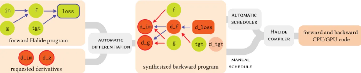
Fig. 3. Overview of our compiler. The user writes a forward Halide program as they would normally. Then, they specify the set of outputs and gradients the system should produce. Our automatic differentiation generates new Halide functions that implement the requested gradients. The user can either manually schedule the pipeline or use our automatic scheduler. Finally, the Halide compiler generates machine code for the scheduled forward and backward algorithms. 4 METHOD

To use our system, a programmer first writes a forward Halide algorithm. They then may request the derivative of some scalar loss with respect to any Halide function, image buffer, or parameter in the pipeline. Our automatic differentiation system visits the graph of functions that describes the forward algorithm and synthesizes new Halide functions that implement the gradient computation (Sec. 4.1). The programmer can either specify the schedule for these new functions manually or use our automatic scheduler (Sec. 4.4). Unlike Halide’s built-in auto-scheduler [Mullapudi et al. 2016], ours recognizes patterns that arise when reversing the computation graph (Sec. 4.2.1). Figure 3 illustrates this workflow.

4.1 High-level strategy

We assume we wish to compute the derivatives of some scalar L, typically a cost function to be minimized. Our system imple-ments reverse-mode automatic differentiation, which computes the gradient with the same time complexity as the forward function (e.g. [Griewank and Walther 2008]). We propagate the adjoints ∂L_∂д to each function in the forward pipelineд, until we reach the inputs. The adjoints of the inputs are the components of the gradient.

Specifically, given a Halide program represented as a graph of Halide functions, we traverse the graph backwards from the output and accumulate contributions to the adjoints using the chain rule. Halide function definitions are represented as expression trees, so within each function we perform a similar backpropagation through the expression tree, propagating adjoints to all leaves.

A key difference between our algorithm and traditional automatic differentiation arises when an expression is a Halide function call. We need to construct a computation which accumulates adjoints onto the called function in the face of non-trivial data dependencies between the two functions. Sec. 4.2 describes this in detail.

We illustrate our algorithm on the simple example in Sec. 3, which performs gamma correction on an image and computes theL2 dis-tance between the output and some target image. To compute the gradients of theL2distance with respect to the input image and the gamma parameter, one would write:

// Obtain gradients with respect to image and gamma parameters

autod_loss_d = propagate_adjoints(loss); Funcd_loss_d_g = d_loss_d(g);

Funcd_loss_d_im = d_loss_d(im);

Throughout the paper, we use the convention that prefixing a function’s name withd_refers to the gradient of that Halide function. We added a key language extension,propagate_adjoints, to Halide. It takes a scalar Halide function and generates gradients in the form of new Halide functions for every Halide function, buffer, and real number parameter the output depends on. Our system can also be used as a component in other automatic differentiation systems that compute gradients. In this case the user can specify a non-scalar Halide function and a buffer representing the adjoints of the function. Figure 3 shows the computational graph for both the forward and backward (gradient) computations.

4.2 Differentiating Halide function calls

A key difference between automatic differentiation in Halide and traditional automatic differentiation is that Halide functions are de-fined on multi-dimensional grids, so function calls and the elements on the grids can have non-trivial aggregate interactions.

Given each input-output pair of Halide functions, we synthesize a new Halide function definition that accumulates the adjoint of the output function onto the adjoint of the input. For performance, we want these new definitions to be as parallelizable as possible.

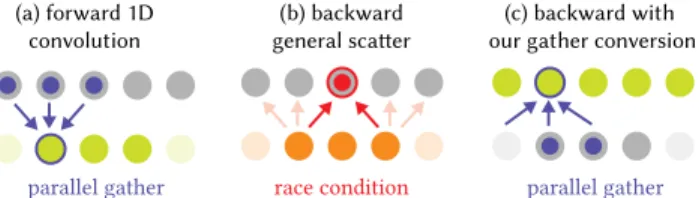
4.2.1 Scatter-gather conversion. Two cases require special care for correctness and efficiency. The first and most important case occurs when each output element reads and combines multiple input values. This happens for example in the simple convolution of Figure 4(a). We call this pattern a gather operation.

When computing gradients in reverse automatic differentiation, the natural reverse of this gather is a scatter operation: each input writes to multiple elements of the output. Scattering operations, however, are not naturally parallelizable since they may lead to race conditions on write. For this reason, we want to convert scatters back to gathers whenever possible. We do this by shearing the itera-tion domain (e.g. [Lamport 1975]). To illustrate this transformaitera-tion, consider the following code that convolves a 1D signal with a kernel, also illustrated in Figure 4(a):

Funcoutput;

output(x) = input(x−r.x) * kernel(r.x);

Assume that we are interested in propagating the gradient toinput. This is achieved by reversing the dependency graph between the input and output variables as shown in Figure 4(b). In code, this transformation would yield:

RDomro;

wherero.xiterates over the originalr.x, andro.yiterates over the domain of output. For each argument in the calls to input, we replace the pure variables (xhere) with reduction variables that iterate over the domain of the output (in this casero.y).r.xis renamed toro.x so we can merge the reduction variables into a single reduction domainro.

This new update definition cannot be computed in parallel overro. ysince multiplero.y− _{ro.xmay write to the same memory location.}

A more efficient way to compute the update, illustrated in Figure 4(c), is to rewrite the same computation as follows:

d_output(x) = select(x >= a && x < b, d_output(x), 0.f); d_input(x) += d_output(x + r.x) * kernel(r.x);

whereaandbare the bounds ofoutput. By shearing the iteration do-main with the variable substitutionx = ro.y− ro.x, we have made d_inputparallelizable overx. Because Halide only iterates over rect-angles, and the sheared iteration domain is no longer a rectangle, we add a zero-padding boundary condition tod_output, and iterate over a conservative bounding box of the sheared domain:

ro.y x

<a

>b

We use Halide’s equation-solving tools to deduce the variable substi-tution to apply. For each argument in a function call, we construct an equation e.g.u = x − rxand solve forx. Importantly, we solve for the smallest interval ofx where the condition holds, since x may map to multiple values. This may introduce new reduction variables, as in the following upsampling operation:

output(x) = input(x/4);

Sincexis an integer, 4 values ininputare used to produce each value ofoutput. Accordingly, our converter will generate the following adjoint code:

RDomr(0, 4); // loops from 0 to 3 d_output(x) = d_input(4*x + r.x)

If any step of this procedure fails to find a solution, we fall back to a general scattering operation. It is still possible to parallelize general scatters using atomics. We added atomic operations to Halide’s GPU backend to handle this case. A general scatter with atomics usually remains significantly less efficient than our transformed code. For instance, the backward pass of a 2D convolution layer applied to a 16 × 16 × 256 × 256 input takes 68 ms using atomics and 6 ms with our scatter-to-gather conversion.

Listing 1 shows some derivatives our system would generate for the bilateral slicing example in the left of Figure 2.

4.2.2 Handling partial updates. The second case which requires special care arises when reversing partial updates to a function. For example, consider the following forward code:

g(x) = f(x);

g(1) = 2.f; // update to f that overwrites a value h(x) = g(x);

When backpropagating the adjoints, we need to propagate correctly through the chain of update definitions. Whileh(x)depends onf(x) for mostx(viag(x)), this is not true forx==1. The update definition toghides the previous dependency onf(1). The corresponding gradient code is:

parallel gather parallel gather

(a) forward 1D convolution

(b) backward general scatter

(c) backward with our gather conversion

race condition

Fig. 4. Our scatter-to-gather conversion enables efficient, parallel code. In this example of a 1D 3-tap convolution, each dot represents a value in the input (resp. output) array. The forward computation (a) produces an output value from three inputs (the faded dots account for boundary conditions). This 3-tap reduction can easily be run in parallel over the output buffer (green dots). Computing the adjoint operator by simply reversing the dependency graph (b), that is by looping in parallel over the output nodes (orange), leads to race conditions since two inputs might need to write to the same location in the input’s adjoint buffer (highlighted in red). This is a common issue with general scattering operations. Using our scatter-to-gather conversion, we convert this backward operation to a reduction overd_out(the adjoint of a convolution is a correlation). In turn, this transformed computation is readily parallelized overd_out’s domain (c).

d_g_update(x) = d_h(x);// Propagate to the first update d_g(x) = d_g_update(x);// Propagate to the initial definition

d_g(1) = 0.f; // Mask unwanted dependency

d_f(x) = d_g(x); // Propagate to f

In general, if we detect different update arguments between two consecutive function updates (in the example above,g(1)is different fromg(x)), we mask the adjoint of the first update to zero using the update argument of the second update.

4.3 Checkpointing

Reverse-mode automatic differentiation on complex pipelines must traditionally deal with a difficult trade-off. Memoizing values from the forward evaluation to be reused in the reverse pass saves com-pute, but costs memory. Even with unlimited memory, bandwidth is limited, so it can be more efficient to recompute values. In automatic differentiation systems this trade-off is addressed with checkpoint-ing [Volin and Ostrovskii 1985], which reduces memory usage by recomputing parts of the forward expressions. However, this is just a specific instance of the general recomputation-vs-memory trade-off already addressed by Halide’s scheduling primitives.

For each function, we can decide whether to create an intermedi-ate buffer for lintermedi-ater reuse (thecompute_root()construct), or recompute values at every call site (thecompute_inline()construct). We can also compute these values at some intermediate granularity, i.e., by set-ting its computation somewhere in the loop nest of their consumers (thecompute_at()construct). Halide also allows checkpointing across different Halide pipelines by using a global cache (thememoize() con-struct). This is useful when the forward pass and backward pass are in separately-compiled units.

As an example, consider the following 2D convolution implemen-tation in Halide:

RDomrk, rt;

convolved(x, y) = 0.f;

convolved(x, y) += in(x− rk.x, y−rk.y) * kernel(rk.x, rk.y); loss() = 0.f;// define an optimization objective

loss() += pow(convolved(rt.x, rt.y)−target(rt.x, rt.y), 2.f); autod = propagate_adjoints(loss);

Listing 1 Derivatives generated by our algorithm for the bilateral slicing code in the left of Fig. 2.

// We start with d_output, which contains the adjoint of output // We propagate the derivatives from d_output to in and affine:

RDomri(0, nci, 0, adjoints.channels()); d_in(x, y, ri.x, n) +=

d_output(x, y, ri.y, n) * affine(x, y, ri.y * (nci + 1), n); d_affine(x, y, ri.y*(nci+1)+ri.x, n) +=

d_output(x, y, ri.y, n) * in(x, y, ri.x, n);

// Variable co is converted into a reduction variable rco.

RDomrco(0, adjoints.channels());

d_affine(x, y, rco*(nci+1)+nci, n) += d_output(x, y, rco, n); // The derivatives are then propagated from affine to grid.

RDomrg(0, 2, 0, 2, 0, 2, 0, sigma_s, 0, sigma_s); Exprinv_x = (x−rg[0]) * sigma_s + rg[3]; Exprinv_y = (y−rg[1]) * sigma_s + rg[4]; d_grid(x, y, fx + rg[2], c) +=

d_affine(inv_x, inv_y, c, n) * d_tent;

// d_tent is tent with (x, y) replaced by (inv_x, inv_y). // The scattering operation is transformed by solving // x == inv_x/sigma_s+rt.x and y == inv_y/sigma_s+rt.y // for inv_x and inv_y.

// Finally, and less obviously, affine also depends on guide.

RDomrgu(0, 2, 0, 2, 0, 2, adjoints.channels()); Exprwxy = abs(rgu[0]−wx) * abs(rgu[1]− wy); Exprwz = select(rgu[2]−wz > 0.f, 1.f, −1.f); d_guide(x, y, n) +=

select(guide(x, y, n) >= 0.f && guide(x, y, n) <= 1.f, d_affine(x, y, rgu[3], c, n)*wxy*wz*grid.channels(), 0.f); We are interested ind_in, the gradient oflosswith respect toin. It is given by a correlation of2*(convolved−target)withkernel, which depends on the values ofconvolved. Using the scheduling handles provided by Halide, we can easily decide whether to cache the values ofconvolvedfor the gradient computation. For example, if we write:

convolved.compute_root();

the values ofconvolvedare computed once and will be fetched from memory when we need them for the derivatived_in. On the other hand, if we write:

convolved.compute_inline();

the values ofconvolvedare computed on-the-fly and no buffer is allocated to store them. This can be advantageous when the con-volution kernel is small (say 2 × 1) since this preserves memory locality, or when the pipeline is much longer and we cannot afford to store every intermediate buffer.

Halide provides scheduling primitives that are more general than binary checkpointing decisions. Fine-grained control over the sched-ule allows exploration of memory/recomputation trade-offs in the forward and gradient code. For instance, we can interleave the com-putation and storage ofconvolvedwith the computation of another Halide function that consumes its value (in this cased_in). The fol-lowing code instructs Halide to compute and store a tile ofconvolved for each 32 × 32 tile ofd_incomputed. This offers a potentially faster balance between computing all ofconvolvedbefore backpropagation, or recomputing each of its pixels on-demand:

d_in.compute_root().tile(x, y, xi, yi, 32, 32);

convolved.compute_at(d_in, x); // compute at each tile of d_in We timed the three schedules above by computingd_in. With multi-threading and vectorization on a CPU, on an image with size of 2560 × 1600 and kernel size 1 × 5, thecompute_inlineschedule takes 5.6 milliseconds while thecompute_rootschedule takes 10.1

milliseconds and thecompute_atschedule takes 9.7 milliseconds. On the same image but with kernel size 3×5, thecompute_inlineschedule takes 66.2 milliseconds while thecompute_rootschedule takes 18.7 milliseconds and thecompute_atschedule takes 12.3 milliseconds. 4.4 Automatic scheduling

Halide’s built-in auto-scheduler [Mullapudi et al. 2016] navigates performance trade-offs well for stencil pipelines, but struggles with patterns that arise when reversing their computational graph (Sec. 4.2.1). In particular, it does not try to optimize large reductions, like those needed to compute a scalar loss. It also does not generate GPU schedules. We therefore implemented a custom automatic scheduler for gradient pipelines.

Similar to Halide’s built-in auto-scheduler, we ask the user to provide an estimate of the input and output buffer sizes. We then infer the extent of all the intermediate functions’ domains.

Our automatic scheduler checkpoints (compute_root) any stage that scatters or reduces, along with those called by more than one other function. We leave any other functions to be recomputed on-demand (compute_inline). For the checkpointed functions, we tile the function domain and parallelize the computation over tiles when possible. Specifically, on CPUs, we split the function’s domain into 2D tiles (16 × 16) and launch CPU threads for each tile, vectorizing the innermost dimension inside a tile. On GPUs, we split the domain into 3D tiles (16 × 16 × 4). The tiles are mapped to GPU blocks, and elements within a tile to GPU threads. In both cases, we tile the first two (resp. three) dimensions of the function’s domain that are large enough. We split the domain if its dimensionality is too low.

If the function’s domain is not large enough for tiling, and the function performs a large associative reduction, we transform it into a parallel reduction using Halide’srfactorscheduling primi-tive [Suriana et al. 2017]. This allows us to factorize the reduction into a set of partial reductions which we compute in parallel and a fi-nal, serial reduction. Like before, we find the first two dimensions of the reduction domain which are large enough for tiling. We reduce the tiles in parallel over CPU threads (resp. GPU blocks). Within each 2D tile, we vectorize (resp. parallelize over GPU threads) the column-wise reductions. We also implemented a multi-level parallel reduction schedule but found it unnecessary in the applications pre-sented. When compiling to GPUs, if both the function domain and the reduction domain are large enough for tiling, but the recursive update does not contain enough pure variables for parallelism, we parallelize the reduction using atomics.

To allow for control over checkpointing, the automatic scheduler decisions can be overridden. We ask the user to provide optional lists of Halide functions they do or do not want to inline. We currently do not usecompute_atin our automatic scheduler.

5 APPLICATIONS & RESULTS

We generate gradients for pipelines in three groups of applications. First, we show that our system can be integrated into existing deep learning systems to more easily develop new, custom operators. Second, we show that we can improve existing image processing pipelines by optimizing their internal parameters on a dataset of training images. Finally, we show how to use our derivatives to solve inverse imaging problems (i.e., optimizing for the image itself).

Unless otherwise specified, we use our automatic scheduler (Sec. 4.4) to schedule all the applications throughout the section (i.e., for both the forward code and the derivatives we generate). Therefore, our implementation only requires the programmer to specify the for-ward pass of the algorithm.

5.1 Custom neural network layers

The class of computations expressible with deep learning libraries such as Caffe [Jia et al. 2014], PyTorch [Paszke et al. 2017], Ten-sorFlow [Abadi et al. 2015], or CNTK [Yu et al. 2014] is growing increasingly rich. Nonetheless, it is still common for a practitioner to require a new, custom node tailored to their problem. For instance, TensorFlow offers a bilinear interpolation layer and a separable 2D convolution layer. However, even a simple extension of these opera-tions to 3D would require implementing a new custom operator in C++ or CUDA to be linked with the main library. This can already be tedious and error-prone. Furthermore, while the forward algorithm is being developed, the adjoint must be re-derived by hand and kept in sync with the forward operator. This makes experimentation and prototyping especially difficult. Finally, both the forward and backward implementations ought to be reasonably optimized so that a model can be trained in a finite amount of time to verify its design.

We implemented a PyTorch backend for Halide so that our deriva-tives can be plugged into PyTorch’s autograd system. We used this backend to re-implement custom operators recently proposed in the literature: the transformation layer in the spatial transformer network [Jaderberg et al. 2015], the warping layer in Flownet 2.0 [Ilg et al. 2017], and the bilateral slicing layer in deep bilateral learn-ing [Gharbi et al. 2017]. The performance of our automatically sched-uled code matches highly-optimized primitives written in CUDA, and is much faster than unoptimized code. We compare the runtime of our method to PyTorch, CNTK, and hand-written CUDA code in Table 1.

5.1.1 Spatial transformer network. The spatial transformer net-work of Jaderberg et al.[2015] applies an affine warp to an interme-diate feature map of a neural network.

The function containing the forward Halide code is 31 lines long excluding comments, empty lines, and function declarations. Due to the popularity of this operator, deep learning frameworks have implemented specialized functions for the layer. The cuDNN li-brary [Chetlur et al. 2014] added its own implementation in version 5 (2016), a year after the original publication. It took another year for PyTorch to implement a wrapper around the cuDNN code. We com-pare our performance to PyTorch’sgrid_sampleandaffine_grid func-tions which use the cuDNN implementation on GPU. On 512 × 512 images with 16 channels and a batch size of 4, our CPU code is around 2.3 times faster than PyTorch’s implementation, and our GPU code is around 20 percent slower than the highly-optimized version implemented in cuDNN. Currently Halide does not sup-port texture sampling on GPU, which could be causing some of the slowdown. We also compare our performance to a CNTK implemen-tation of spatial transformer using the gather operation. Our GPU code is around 10 times faster than the CNTK implementation.

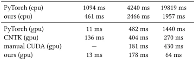
Table 1. Performance of our approach for custom neural network operators. The runtime measures end-to-end latency for forward+backward evaluation. The spatial transformer transforms a batch of 4×16×512×512. The Flownet node warps a batch of 4×64×512×512 images with a 2D warping field. The BilateralSlice layer processes images with size 4 × 4 × 1024 × 1024 and grid size 4 × 12 × 64 × 64. Measurements were made on an Intel Core i7-3770K CPU @ 3.50GHz, with 16GB of RAM and a NVIDIA Titan X (Pascal) GPU with 12 GB of RAM.

operator SpatialTransformer Flownet BilateralSlice

PyTorch (cpu) 1094 ms 4240 ms 19819 ms

ours (cpu) 461 ms 2466 ms 1957 ms

PyTorch (gpu) 11 ms 482 ms 1440 ms

CNTK (gpu) 136 ms 404 ms 270 ms

manual CUDA (gpu) — 181 ms 430 ms

ours (gpu) 13 ms 178 ms 64 ms

Having fixed functions such asaffine_gridcan be problematic when users want to slightly modify their models and experiment with different ideas. For example, changing the interpolation scheme (e.g., bicubic or Lanczos instead of bilinear), or interpolating over more dimensions (e.g., transforming volume data) would require implementing a new custom operator. Using our system, these mod-ifications only require minor code changes to the forward algorithm. Our system then generates the derivatives automatically, and our automatic scheduler provides performance without further effort.

5.1.2 Warping layer. FlowNet 2.0 [Ilg et al. 2017], which targets optical flow applications, introduced a new 2D warping layer. Com-pared to the previous spatial transformer layer, this warping layer is a more general transform using a per-pixel warp-field instead of a parametric transformation.

The function containing the forward Halide code is 18 lines long. The original warping function was implemented as a custom node in Caffe. The authors had to write the forward and reverse code for both the CPU and GPU backends. In total it comprises more than 400 lines of code1. While the custom node can handle 2D warps well, adapting it to higher-dimensional warps or semi-parametric warps would be challenging. Our system makes this much easier. In addition to PyTorch and CNTK, we also compare the performance of our GPU code with a highly-optimized reimplementation from NVIDIA2. The performance of our code is comparable to the highly-optimized CUDA code.

5.1.3 Bilateral slicing layer. Deep bilateral learning [Gharbi et al. 2017] is a general, high-performance image processing architecture inspired by bilateral grid processing and local affine color trans-forms. It can be used to approximate complicated image processing pipelines with high throughput. The algorithm works by splatting a 2D image onto a 3D grid using a convolutional network. Each voxel of the grid contains an affine transformation matrix. A high-resolution guidance map is then used to slice into the grid and produce a unique, interpolated, affine transform to apply to each 1_{FlowNet 2.0: https://github.com/lmb-freiburg/flownet2/blob/master/src/caffe/layers/} flow_warp_layer.cu

input pixel. The original implementation in TensorFlow had to im-plement a custom node1for the final slicing operation due to the lack of an efficient way to perform trilinear interpolation on the grid. This custom node also applies the affine transformation on the fly to avoid instantiating a high-resolution image containing all the affine parameters at each pixel. The reference custom node had around 300 lines of CUDA code excluding comments and empty lines. Using the recently introduced general scattering functionality, we can implement the same operation directly in PyTorch. Figure 2 shows a comparison between our Halide code, reference CUDA code, and PyTorch code.

The PyTorch and CNTK implementations are modestly more complex than our code. PyTorch is 20 times slower while CNTK is 4 times slower on an 1024 × 1024 input with a grid size of 32 × 32 × 8 and a batch size of 4. CNTK is faster than PyTorch due to different implementation choices on the gather operations. The manual CUDA code aims for clarity more than performance, but is both more complicated and 6.7 times slower than our code.

Gharbi et al. [2017] argue that training on high resolution im-ages is key to capturing the high frequency features of the image processing algorithm being approximated. Both the PyTorch and CNTK code run out of memory on a 2048 × 2048 input with grid size 64 × 64 × 8 on a Titan GPU with 12 GB of memory. This makes it almost impossible to experiment with high-resolution inputs. Our code is 13.7 times faster than the authors’ reference implementation on this problem size.

5.2 Parameter optimization for image processing pipelines Traditionally, when developing an image processing algorithm, a programmer manually tunes the parameters of their pipeline to make it work well on a small test set of images. When the num-ber of parameters is large, manually determining these parameters becomes very difficult.

In contrast, modern deep learning methods achieve impressive results by using a large number of parameters and many training images. We demonstrate that it is possible to apply a similar strategy to general image processing algorithms, by augmenting the algo-rithm with more parameters, and tuning these parameters through an offline training process. Our system provides the necessary gra-dients for this optimization. Users write the forward code in Halide, and then optimize the parameters of the code using training images. We demonstrate this with an image demosaicking algorithm based on the adaptive homogeneity-directed demosaicking of Hirakawa and Parks [2005], and a non-blind image deconvolution algorithm based on the sparse adaptive priors proposed by Fortunato and Oliveira [2014].

5.2.1 Image demosaicking. Demosaicking seeks to retrieve a full-color image from incomplete full-color samples captured through a color filter array, where each pixel only contains one out of three red, green and blue colors. Traditional demosaicking algorithms work well on most cases, but can exhibit structured aliasing arti-facts such as zippering and moiré (Figure 5). Recent methods using deep learning have achieved impressive results [Gharbi et al. 2016], 1_{https://github.com/mgharbi/hdrnet/blob/master/hdrnet/ops/bilateral_slice.cu.cc}

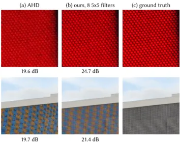
(a) AHD

19.6 dB 24.7 dB

19.7 dB 21.4 dB

(b) ours, 8 5x5 filters (c) ground truth

Fig. 5. We use our automatic gradients to relax the AHD demosaicking algorithm (a) by adding more filters to interpolate the green channel (8 instead of 2 here, with 5x5 footprint instead of 5x1). With this simple tweak, and by optimizing the filters using our automatically generated derivatives, we can obtain sharper images in difficult cases (b), first row. The small-footprint of this simple demosaicking method nevertheless inherits some of the limitations of AHD. In particular, it leads to artifacts in complex, moiré-prone patterns (second row). Images taken from deep demosaicking dataset [Gharbi et al. 2016].

Table 2. PSNR for several demosaicking techniques following the evaluation methodology of Gharbi et al. (higher is better). We implemented a version of Hirakawa et al.’s AHD demosaicking algorithm with our system. Despite the simplicity of our approach, by relaxing the algorithm’s specifications (i.e. adding more filters on the green channel reconstruction with larger foot-prints) and re-optimizing the parameters, we achieve higher fidelity (over 1 dB better) for a similar computational cost. While our method does not rival state-of-the-art deep-learning-based techniques, it is significantly faster and opens up new avenues to optimize more parsimoniously parametrized algorithms tailored to the problem. (Timings reported for a 1 megapixel image. (*)Timing for these algorithms is from non-optimized MATLAB code.)

kodak mcm vdp moiré time

bilinear 32.9 32.5 25.2 27.6 *127ms

Adobe Camera Raw 9 33.9 32.2 27.8 29.8 —

AHD Hirakawa [2005] 36.1 33.8 28.6 30.8 *1618ms

ours (2 filters, 5x5) 36.7 34.7 29.4 31.5 71ms

ours (9 filters, 5x5) 36.8 35.2 29.8 31.7 177ms

ours (15 filters, 7x7) 37.3 35.5 30.1 32.0 324ms

Gharbi [2016] 41.2 39.5 34.3 37.0 2932ms

however, the execution time is still an issue for practical usage. We relax the adaptive homogeneity-directed demosaicking algorithm (AHD) [Hirakawa and Parks 2005], variations of which are the de-fault algorithms in Adobe Camera Raw and dcraw. We increase the number of filters to interpolate the green channel. We also fine-tune the chrominance (red-blue) interpolation filters from the AHD ref-erence. We experiment with different number of filters and filter sizes to explore the runtime versus accuracy trade-off. We optimized

blurred ground truth

Fortunato 2014 (25.39 dB) ours (27.37 dB)

Fig. 6. We use automatic gradients to enhance Fortunato and Oliveira’s non-blind deconvolution algorithm [2014]. We use more iterations and automatically train the weights, thresholds and filtering parameters. We are able to get sharper results. On eight randomly selected-images we achieve an average PSNR of 29.57 dB. Using the original algorithm with its original parameters the PSNR is 28.51 dB. Image taken from ImageNet [Deng et al. 2009]

the filter weights on Gharbi et al.’s [2016] training dataset using the gradients provided by our system. The results are illustrated in Table 2. With this simple modification, we obtain a significant 1 to 1.5 dB improvement on the more difficult datasets (moiré and vdp), depending on the number of filters used. We also obtain visually sharper images on many challenging cases, as shown in Figure 5.

With its limited footprint and filtering complexity, our optimized demosaicking still struggles on moiré-prone textures. Our system will allow users to experiment with more complex ideas without having to implement the derivatives at each step. For instance, we were able to quickly experiment with (and ultimately discard) al-ternative algorithms (e.g. using filters that take the ratio between colors into account and 1D directional filters).

5.2.2 Non-blind image deconvolution. The task of non-blind im-age deconvolution is: given a point spread function and a blurry image, which is the result of a latent natural image convolved with the function, recover the underlying image. The problem is highly ill-posed, therefore the quality of the reconstruction heavily depends on the priors we place on the image. It is thus important to learn a good set of parameters for those priors.

We based our implementation on the sparse adaptive prior pro-posed by Fortunato and Oliveira [2014]. The original method works in a 2-stage fashion. In the first stage they solve a conventionalL2

(a) our output R (b) dcraw (AHD) single frame

(c) [Gharbi 2016] single frame Fig. 7. Automatic gradients can be used for inverse problems such as high-resolution demosaicking from a burst of images. The user only needs to implement the forward model. Bursts of RAW images are captured with a Nikon D810camera then jointly aligned and demosaicked (13 and 23 images respectively, only showing crops). We initialize our recontruction to a simple bilinear interpolation (not shown) and solve an inverse problem to recover both a set of homographies and a demosaicked image that matches the captured data when reprojected. Compared to the result of dcraw’s AHD algorithm (a) and Gharbi et al. [2016] (c), our output (b) is much sharper, and shows less noise (red square) and color moiré (green square).

deconvolution using a set of discrete derivative filters as the prior. Then they use an edge-aware filter to cleanup the noise in the image. In the second stage, anotherL2deconvolution is solved for large discrete derivatives by matching the prior terms to the result of the first stage, masked by a smooth thresholding function.

We extend the method by increasing the number of stages (we use 4 instead of 2), and having a different set of filters for the priors for each stage. We optimize the weights of the prior filters, the smoothness parameters of the edge-aware filter (we use a bilateral grid), and the thresholding parameters in the smooth thresholding functions.

To demonstrate the ability of our system to handle nested deriva-tives, we implemented a generic non-linear conjugate gradient solver using a linear search algorithm based on Newton-Raphson to solve for theL2deconvolution. We write the conjugate gradient loop in PyTorch, but implement the gradient and vector-Hessian-vector product (required in the line search step) in Halide. We also imple-mented the bilateral grid filtering step in Halide. To optimize the parameters, we then differentiate through the gradients we used for the non-linear conjugate gradient algorithm. We train our method on ImageNet [Deng et al. 2009] and use the point spread function generation scheme described in Kupyn et al.’s work [2017]. We ini-tialize the parameters to the recommended parameters described in Fortunato and Oliveira’s work. Figure 6 shows the result.