Driving segments analysis for energy and environmental impacts of worsening traffic

(1)

DRIVING SEGMENTS ANALYSIS FOR ENERGY AND ENVIRONMENTAL IMPACTS OF WORSENING TRAFFIC

by

Wen Feng

B.S. Refrigeration and Cryogenics Engineering Shanghai Jiao Tong University, Shanghai, China, 2000

M.S. Thermal Engineering Tsinghua University, Beijing, China, 2003 Submitted to the Engineering Systems Division and the Department of Civil and Environmental Engineering in Partial Fulfillment of the Requirements for the Degrees of

Master of Science in Technology and Policy and Master of Science in Civil and Environmental Engineering

at the

Massachusetts Institute of Technology June 2007

Signature of Author………... Technology and Policy Program, Engineering Systems Division Department of Civil and Environmental Engineering May 11th, 2007 Certified by.………

David H. Marks

Morton and Claire Goulder Family Professor of Civil and Environmental Engineering and Engineering Systems Co-Director, MIT Laboratory for Energy and the Environment Thesis Supervisor Certified by.……… Stephen R. Connors Director, Analysis Group for Regional Energy Alternatives Thesis Supervisor Accepted by...……….……

Daniele Veneziano

Professor of Civil and Environmental Engineering Chairman, Departmental Committee on Graduate Students Accepted by………...……….……

Dava J. Newman

Professor of Aeronautics and Astronautics and Engineering Systems Director, Technology and Policy Program

(2)

(3)

DRIVING SEGMENTS ANALYSIS FOR ENERGY AND

ENVIRONMENTAL IMPACTS OF WORSENING TRAFFIC

by

Wen Feng

Submitted to the Engineering Systems Division and the Department of Civil and Environmental Engineering on May 11th, 2007 in Partial Fulfillment of the Requirements for the Degrees of Master of Science in Technology and Policy and Master of Science in Civil and Environmental Engineering

ABSTRACT

During the last two decades, traffic congestion in the U.S. has increased from 30% to 67% of peak period travel. Further, current research shows that measures taken within transportation systems, such as adding capacity, improving operations and managing demand, are not enough to keep congestion from growing worse. With the worsening traffic, the vehicle’s fuel consumption and pollutant emissions will inevitably increase. As such, this thesis aims to quantitatively evaluate the energy and environmental impacts of worsening traffic on individual vehicles and the U.S. light-duty vehicle fleet, as well as to design feasible measures beyond transportation systems to offset theses impacts.

The fuel consumption and emissions of different vehicle types under different driving situations provide the basis for analyzing the energy and environmental impacts of worsening traffic. This thesis defines the concept of “driving segments” to represent all possible driving situations which consist of vehicle speed, operation patterns and road types. For each vehicle type, its fuel consumption and emissions in different “driving segments” can be developed into a matrix by ADVISOR 2004, the vehicle simulation tool.

Combining the “driving segments” vehicle performance matrices with the model for traffic congestion, the energy and environmental impacts of worsening traffic on individual vehicles can be examined. Based on these impacts, this thesis compares the performance of different vehicle types for both today’s and tomorrow’s traffic situations. Meanwhile, the on-road fuel economy of each vehicle type has also been calculated to update EPA’s fuel economy rating by taking worsening traffic into consideration.

Combining the “driving segments” vehicle performance matrices with a set of models for fleet population, vehicle technology, driving behavior and traffic congestion, the energy and environmental impacts of worsening traffic on the U.S. light-duty vehicle fleet can

(4)

also be examined. Through sensitivity analysis, this thesis investigates the effects of altering vehicle choice, developing vehicle technology and changing driving behavior on offsetting the fuel consumption and emissions of the U.S. light-duty vehicle fleet caused by worsening traffic through 2030. It is concluded that promoting the market share of advanced vehicle technologies (Hybrids mainly) is the most effective and most feasible method.

Thesis Supervisor: David H. Marks

Morton and Claire Goulder Family Professor of

Civil and Environmental Engineering and Engineering Systems

Co-Director, MIT Laboratory for Energy and the Environment

Thesis Supervisor: Stephen R. Connors

Director, Analysis Group for Regional Energy Alternatives

(5)

ACKNOWLEDGEMENTS

I would like to extend my deepest thanks to Prof. David Marks and Mr. Stephen Connors, my two thesis supervisors. Acting as the distinguished leader of the Laboratory for Energy and the Environment, Prof. Marks is the person who attracted me to MIT three years ago and since then he has given me enormous help in both my life and study. Meanwhile, Mr. Connors is the person who influences me most on my research. From the early days of elaborating the research question to the final stages of thesis proofreading, Mr. Connors has always been a source of inspiration and invaluable guidance.

I would like to extend my sincere thanks to the faculty, staff and students from the ESD / TPP / LFEE: Prof. Joseph Sussman, to whom I owe a tremendous debt of gratitude for his insightful advice on my research topic; Prof. Dava Newman, Dr. Frank Field and Ms. Sydney Miller, for their charming personalities, great patience, warm encouragement and countless help as well as for making TPP such a successful program; Ms. Jackie Donoghue, for her decades of dedication to the LFEE researchers; and so on. I also need to thank all my friends at MIT and elsewhere for their wonderful friendship which makes my life valuable and enjoyable.

I would like to extend my special thanks to MIT alumni, Mr. Derry Kabcenell (EE '75) and Ms. Charlene Kabcenell (EE '79) for establishing the Kabcenell Future Energy Fellowship. Their generous support makes this exciting research possible.

Finally, I would like to dedicate this thesis to my parents for providing me endless courage to surmount all the difficulties on my way. Without their love, I would have never made it this far.

(6)

(7)

LIST OF TABLES

Table 2-1: LOS and Basic Assumptions………27

Table 2-2: Comparison for Vehicle Simulation Tools………31

Table 2-3: Vehicle Classification and Simulation Parameters………...35

Table 2-4: “V-A” Performance Matrix for Two-seater Car (Automatic Transmission)….37 Table 2-5: “Driving Segments” Vehicle Performance Matrix for Two-seater Car (Automatic, Free Flow, Time)………..…….38

Table 2-6: “Driving Segments” Vehicle Performance Matrix for Two-seater Car (Automatic, Free Flow, Mileage)………..………39

Table 3-1: Three Sets of Driving Situations………...43

Table 3-2: Traffic Assumptions for 2005 and 2010………...45

Table 3-3: Velocity-Acceleration Matrices for Compact Sedan………47

Table 3-4: “Per-Trip” Fuel Consumption and Emissions of Compact Sedan………48

Table 3-5: Annual Morning Commute Fuel Consumption and Emissions of Compact Sedan………..…...48

Table 3-6: “On-road” Fuel Economy for Work Commute in 2010 (MPG)………...53

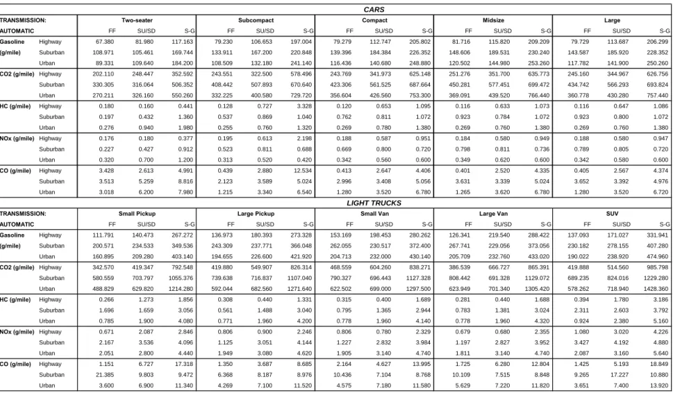
Table 3-7: “Driving Segments” Vehicle Performance Inventory for Cars and Light Trucks (Automatic Transmission)……….57

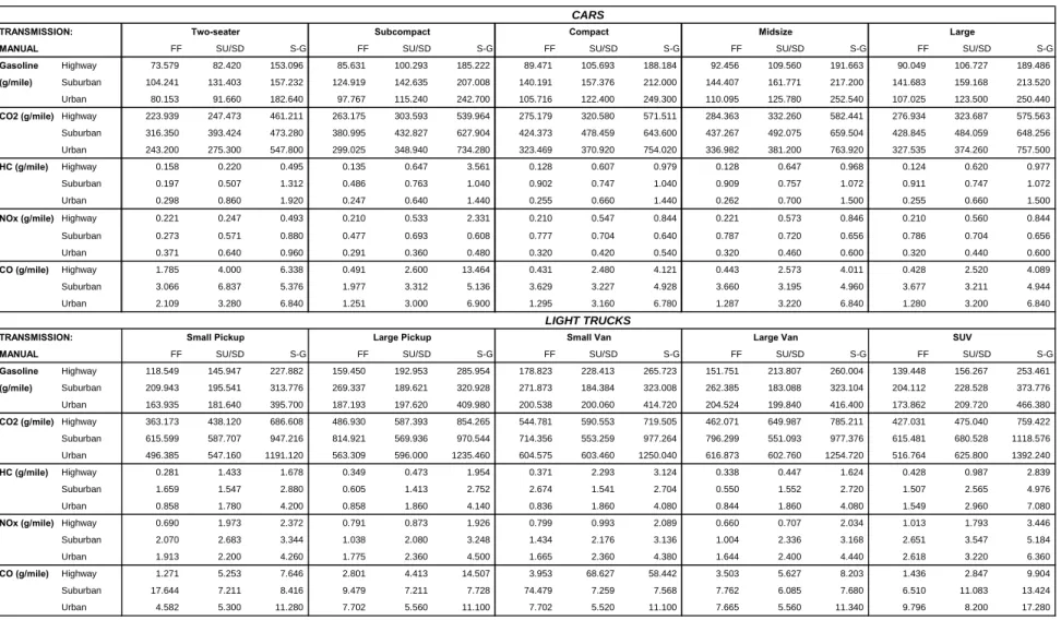
Table 3-8: “Driving Segments” Vehicle Performance Inventory for Cars and Light Trucks (Manual Transmission)………...…..58

Table 3-9: “Driving Segments” Vehicle Performance Inventory for New Tech…………59

Table 4-1: Three Versions for Vehicle Classification……….73

Table 4-2: Baseline Characteristics Inventory (cars and light trucks with automatic transmission, MY 2000 & 0-year-old)………..76

Table 4-3: Baseline Characteristics Inventory (cars and light trucks with manual transmission, MY 2000 & 0-year-old)……….……….77

Table 4-4: Baseline Characteristics Inventory (new technologies, automatic = manual)..78

Table 4-5: Average Speed on Three Road Types (mph)……….83

Table 4-6: Definition of Static Case and Base Cases……….95

Table 4-7: Case Scenarios and Impacts Analysis………...96

Table 4-8: Six Groups of Sensitivity Analysis for the Reference Case (14 Scenarios)...105

Table 4-9: Impact Ranks for 14 Scenarios of Sensitivity Analysis (Worst to Best)…….114

Table 4-10: Description of Offset Methods………..115

(11)

LIST OF FIGURES

Figure 1-1: Definition for Sustainable Mobility………...16

Figure 1-2: Relationship between Traffic Congestion and Energy Consumption / Environmental Pollution....……….………16

Figure 1-3: The Change of Traffic Congestion in the U.S……….19

Figure 1-4: Conceptual “Driving Segments”……….21

Figure 1-5: “Driving Segments” Methodology………..22

Figure 2-1: Velocity-Acceleration (V-A) Graph………26

Figure 2-2: Driving Situations and “Driving Segments” (Highway)……….28

Figure 2-3: Driving Situations and “Driving Segments” (Suburban Road)………...28

Figure 2-4: Driving Situations and “Driving Segments” (Urban Street)………...29

Figure 2-5: Three Sample “Driving Segments” on Highway………30

Figure 2-6: V-A Distribution for ARB02………..36

Figure 2-7: V-A Distribution for CSHVR……….36

Figure 2-8: V-A Distribution for FTP………36

Figure 2-9: V-A Distribution for LA-92……….………36

Figure 2-10: V-A Distribution for IDLING………....36

Figure 2-11: V-A Distribution for INRETS………...36

Figure 2-12: V-A Distribution for OCC……….37

Figure 3-1: Driving Situation Description (Velocity-Distance)……….44

Figure 3-2: Driving Situation Description (Velocity-Time)………...44

Figure 3-3: Traffic Assumptions for 2005 and 2010………..45

Figure 3-4: Velocity-Acceleration Graph for Vehicle Performance………...47

Figure 3-5: Annual Fuel Consumption Change in 2010………49

Figure 3-6: Annual CO2 Emission Change in 2010………...49

Figure 3-7: Annual HC Emission Change in 2010………49

Figure 3-8: Annual NOX Emission Change in 2010………..49

Figure 3-9: Annual CO Emission Change in 2010………49

Figure 3-10: Annual Fuel Percentage Change in 2010………..50

Figure 3-11: Annual CO2 Percentage Change in 2010………...50

Figure 3-12: Annual HC Percentage Change in 2010………50

Figure 3-13: Annual NOX Percentage Change in 2010………..50

Figure 3-14: Annual CO Percentage Change in 2010………50

(12)

Figure 3-16: Annual Fuel Cost in 2010 ($2.0 / gallon)………..52

Figure 3-21: Comparison between “On-road” and “FEG” Fuel Economy………54

Figure 3-22: Percentage Composition of Congestion Levels (1982-2003)………...60

Figure 3-23: Fuel Consumption Change (Automatic)………...60

Figure 3-24: Fuel Consumption Change (Manual)………60

Figure 3-25: CO2 Emission Change (Automatic)………..60

Figure 3-26: CO2 Emission Change (Manual)………...60

Figure 3-27: HC Emission Change (Automatic)………61

Figure 3-28: HC Emission Change (Manual)………61

Figure 3-29: NOX Emission Change (Automatic)……….61

Figure 3-30: NOX Emission Change (Manual)………..61

Figure 3-31: CO Emission Change (Automatic)………61

Figure 3-32: CO Emission Change (Manual)………61

Figure 3-33: Fuel Economy Change (Automatic)………..63

Figure 3-34: Fuel Economy Change (Manual)………..63

Figure 3-35: Value Comparison between “On-road” and “FEG” Fuel Economy………..63

Figure 3-36: Percentage Comparison between “On-road” and “FEG” Fuel Economy….63 Figure 4-1: Linear Extrapolation and Sale Shares of Two-seater Cars………..70

Figure 4-2: Linear Extrapolation and Sale Shares of Subcompact Cars………70

Figure 4-3: The U.S. Light-Duty Vehicle Fleet Stock (Version 2)……….73

Figure 4-4: Population Composition of the U.S. Light-Duty Vehicle Fleet (Version 2)…74 Figure 4-5: Fuel Economy of the U.S. Light-Duty Vehicles……….79

Figure 4-6: Correlation Coefficients for Fuel Economy………79

Figure 4-7: Deterioration Rate for Fuel Economy……….80

Figure 4-8: The Change of Transmission Methods for Passenger Cars……….81

Figure 4-9: The Change of Transmission Methods for Light Trucks………82

Figure 4-10: The Change of Road Type Composition in Vehicle Usage………...84

Figure 4-11: The Change of Average Driving Speed……….84

Figure 4-12: The Change of Vehicle Usage with Time (1982-2001)……….85

Figure 4-13: The Change of Vehicle Usage with Aging (Estimated in 2001)…………...85

Figure 4-14: Percentage Composition of Congestion Levels………87

(13)

Figure 4-16: Percentage Composition of the U.S. LDV Fleet Fuel Consumption (Version 2)………....89 Figure 4-17: CO2 Emission of the U.S. Light-Duty Vehicle Fleet (Version 2)…………..90

Figure 4-18: Percentage Composition of the U.S. LDV Fleet CO2 Emission (Version

2)………....90 Figure 4-19: HC Emission of the U.S. Light-Duty Vehicle Fleet (Version 2)…………...91 Figure 4-20: Percentage Composition of the U.S. LDV Fleet HC Emission (Version 2)..91 Figure 4-21: NOX Emission of the U.S. Light-Duty Vehicle Fleet (Version 2)………….92

Figure 4-22: Percentage Composition of the U.S. LDV Fleet NOX Emission (Version

2)………..…..92 Figure 4-23: CO Emission of the U.S. Light-Duty Vehicle Fleet (Version 2)…………...93 Figure 4-24: Percentage Composition of the U.S. LDV Fleet CO Emission (Version 2)..93 Figure 4-25: Percentage Composition for Vehicle Population, Fuel Consumption and

Emissions in 2030……….…94 Figure 4-26: Impacts Analysis for Fuel Consumption of the U.S. Light-Duty Vehicle

Fleet………...97 Figure 4-27: Impacts Analysis for Fuel Consumption in 2030 (Change to Static Case)...97 Figure 4-28: Impacts Analysis for CO2 Emission of the U.S. Light-Duty Vehicle Fleet...98

Figure 4-29: Impacts Analysis for CO2 Emission in 2030 (Change to Static Case)……..98

Figure 4-30: Impacts Analysis for HC Emission of the U.S. Light-Duty Vehicle Fleet…99 Figure 4-31: Impacts Analysis for HC Emission in 2030 (Change to Static Case)……...99 Figure 4-32: Impacts Analysis for NOX Emission of the U.S. Light-Duty Vehicle

Fleet……….100 Figure 4-33: Impacts Analysis for NOX Emission in 2030 (Change to Static Case)…...100

Figure 4-34: Impacts Analysis for CO Emission of the U.S. Light-Duty Vehicle Fleet..101 Figure 4-35: Impacts Analysis for CO Emission in 2030 (Change to Static Case)…….101 Figure 4-36: Percentage Composition of Congestion Levels (Reference Case: Worse)..105 Figure 4-37: Percentage Composition of Congestion Levels (Sensitivity Analysis 3.1:

Half Worse)……….106 Figure 4-38: Percentage Composition of Congestion Levels (Sensitivity Analysis 3.2:

Same with 2003)………..106 Figure 4-39: Percentage Composition of Congestion Levels (Sensitivity Analysis 3.3:

Half Better)………..107 Figure 4-40: Percentage Composition of Congestion Levels (Sensitivity Analysis 3.4:

Better)………..107 Figure 4-41: Sensitivity Analysis for Fuel Consumption……….109

(14)

Figure 4-42: Sensitivity Analysis for CO2 Emission………110

Figure 4-43: Sensitivity Analysis for HC Emission……….111

Figure 4-44: Sensitivity Analysis for NOX Emission………...112

Figure 4-45: Sensitivity Analysis for CO Emission……….113

Figure 4-46: Offset Analysis for Fuel Consumption………117

Figure 4-47: Offset Analysis for CO2 Emission………...118

Figure 4-48: Offset Analysis for HC Emission………118

Figure 4-49: Offset Analysis for NOX Emission………..119

Figure 4-50: Offset Analysis for CO Emission………119

Figure 4-51: Half-Worst Traffic Congestion………120

Figure 4-52: Additional Sensitivity Analysis for Fuel Consumption………...122

Figure 4-53: Additional Sensitivity Analysis for CO2 Emission………..122

Figure 4-54: Additional Sensitivity Analysis for HC Emission………...123

Figure 4-55: Additional Sensitivity Analysis for NOX Emission……….123

Figure 4-56: Additional Sensitivity Analysis for CO Emission………...124

Figure 4-57: Gasoline Prices………127

Figure 4-58: Carbon Prices………..128

Figure 4-59: Total Benefits from Gasoline and Carbon Savings (by Offset Method 1)..129

Figure 4-60: Percentage Composition of Total Benefits in 2030 (by Offset Method 1)..129

Figure 4-61: “Iso-Benefits” Curves in 2030 (2004 US $, by Offset Method 1)………..130

Figure 4-62: The U.S. Petroleum Imports from the Middle East………132

Figure 4-63: Market Penetration of New Vehicle Technologies (Scenario 1)………….134

Figure 4-64: Petroleum Savings from New Vehicle Technologies (Scenario 1)………..134

Figure 4-66: Petroleum Savings from New Vehicle Technologies (Scenario 2)………..135

(15)

CHAPTER 1: INTRODUCTION

1.1 Motivation

The invention of the petroleum-fueled motor vehicle at the end of 19th century was the prologue for the “golden age” of mobility by improving accessibility, and driving economic development. But in less than one hundred years, the world has also suffered a variety of negative impacts associated with motor mobility, such as traffic congestion, energy shortages, environmental pollution, car accident, etc. In light of the general rules of sustainability, more and more researchers are trying to identify ways to mitigate these negative impacts, while enhancing the positive impacts of mobility in order to achieve “sustainable mobility” (see Figure 1-1), which means the ability to meet the needs of society to move freely, gain access, communicate, trade, and establish relationships without sacrificing other essential human or ecological values today or in the future [WBCSD, 2001].

However, current research on sustainable mobility tends to study traffic congestion, energy consumption and environmental pollution separately and the relationship between these impacts on mobility is often overlooked (see Figure 1-1). Vehicle fuel consumption and emissions are determined by both vehicle technologies and real-world driving situations, such as driving behavior and traffic congestion (see Figure 1-2). When traffic congestion becomes worse, vehicle driving situations will change from “free flow” to “speed up/slow down” and even to “stop-and-go”, and such changes will cause more fuel to be wasted through non-productive engine operation [TTI, 2005] and more emissions [Dodder, 2006]. In other words, worsening traffic will acerbate energy consumption and environmental pollution through changing the driving situations for all motor vehicles.

(16)

Figure 1-1: Definition for Sustainable Mobility [Adapted from WBCSD, 2001]

Figure 1-2: Relationship between Traffic Congestion and Energy Consumption / Environmental Pollution

Based on the above qualitative analysis, it would be a pressing task for us to quantify the energy and environmental impacts of worsening traffic, i.e., the increase of vehicle fuel consumption and emissions when traffic congestion becomes worse. There are three major reasons why this task is so important:

First of all, quantifying the energy and environmental impacts of worsening traffic can help us fully understand the relationship between traffic congestion, energy consumption and environmental pollution. The additional fuel consumption and emissions caused by worsening traffic in the past can be identified. And if traffic congestion becomes continuously worse in the future, its impacts on energy and the environment can also be projected and taken as a reference for policy makers.

– Environ- & Eco- Sys.

+ Mobility’s Impacts Economy Congestion Pollution Safety Sustainable Mobility

The ability to meet the needs of society to move freely, gain access, communicate, trade, and establish relationships without sacrificing other essential human or ecological values today or in the future. + – Proper Infrastructure Freight Transportation Traffic Congestion Use of Fossil Energy

Traffic Accidents

General Rules for Sustainability Access and Equity

Accessibility

Energy Shortage / Environmental Pollution

Vehicle Fuel Consumption / Emissions

Real-world Driving Situations

Vehicle Technologies

Traffic Congestion

(17)

Second, quantifying the energy and environmental impacts of worsening traffic can help us design feasible measures beyond transportation systems to “offset” these impacts. On one hand, existing research shows that measures taken within transportation systems such as adding road capacity, improving operations and managing demand are not enough to keep congestion from growing worse in many countries and areas [TTI, 2005], and therefore it’s necessary to find the measures outside of transportation systems to mitigate the energy and environmental impacts of worsening traffic. On the other hand, qualitative analysis indicates that vehicle fuel consumption and emissions are influenced by not only traffic congestion but also vehicle technologies and driving behavior (see Figure 1-2), and thus it’s also reasonable to offset the increase of fuel consumption and emissions caused by worsening traffic through some measures beyond transportation systems, such as altering vehicle choices, developing vehicle technologies or changing driving behavior.

Last but not least, quantifying the energy and environmental impacts of worsening traffic can help us better calculate the “on-road” fuel economy to compare the real performance of different vehicle technologies for both today’s and tomorrow’s traffic situations. Since the 1970s, the fuel consumption and emissions of motor vehicles have been always tested under standard “driving cycles” (series of data points representing the speed of a vehicle versus time) [ISO, 2003], which unfortunately no longer represent the real-world driving situations [Samuel et al., 2003]. However, once the energy and environmental impacts of worsening traffic are quantified, the limitations of standard driving cycles can be overcome and it will be straightforward to quantify the performance of different vehicle types under any traffic situation.

All in all, quantifying the energy and environmental impacts of worsening traffic is a very necessary and important task for sustainable mobility research. Accomplishing this task is exactly the motivation of this thesis.

(18)

1.2 Scope

In order to make a reasonable simplification for the above task while still developing a general framework to quantify the energy and environmental impacts of worsening traffic, this thesis limits its scope on the following two aspects:

First, the U.S. road transportation system from 1982 to 2030 defines the space and time domains to model worsening traffic. During the last two decades, the worst congestion levels (including “Severe” and “Extreme”) in the U.S. have increased from 12% to 40% and free-flowing travel in 2003 is less than half of the amount in 1982 (see Figure 1-3), and this trend is forecasted to continue in the future 25 years [TTI, 2005]. Moreover, almost one third of the world’s total motor vehicles is in the U.S. and so will be influenced by changing traffic situations [Ward’s Communications, 2004]. Therefore the U.S. road transportation system provides a meaningful backdrop to describe how the traffic congestion became worse in the past, as well as how it might worse in the future.

Second, the U.S. light-duty vehicles and their fleet are taken as the object to study the energy and environmental impacts of worsening traffic. In fact, nearly 96% of the U.S. motor vehicles are light-duty vehicles (passenger cars and light trucks with gross weight under 10,000 pounds) [ORNL, 2005], and these light-duty vehicles account for 80% of the U.S. road transportation fuel consumption (equivalent to 39% of the U.S. total petroleum consumption or 16% of the U.S. total energy consumption) and 22% of the U.S. total CO2 emissions [Bassene, 2001; EIA, 2005]. Therefore, by looking at the

light-duty vehicle fleet we capture a majority of road vehicle transportation, and a sizable fraction of national energy consumption and emissions.

(19)

Figure 1-3: The Change of Traffic Congestion in the U.S. [TTI, 2005]

1.3 Objectives

Considering both motivation and scope of this thesis as described above, the objectives of this thesis include:

1) Developing a general framework or methodology to quantify the energy and environmental impacts of worsening traffic;

2) Identifying the additional fuel consumption and emissions of passenger cars and light trucks as well as the U.S. light-duty vehicle fleet caused by worsening traffic in the last two decades;

3) Estimating the energy and environmental impacts of future traffic congestion on the U.S. light-duty vehicle fleet and designing feasible measures beyond transportation systems to offset these impacts;

(20)

4) Calculating the on-road fuel economy of light-duty vehicles to improve EPA’s outdated fuel economy rating and to compare the real performance of different vehicle types for both today’s and tomorrow’s traffic congestion levels;

5) Suggesting policy alternatives to improve the energy and environmental performance of light-duty vehicles under different traffic situations.

1.4 Methodology

As illustrated in Figure 1-2, the energy and environmental impacts of worsening traffic can be quantified if worsening traffic can be modeled and combined with vehicle fuel consumption and emissions estimates under a wide variety of driving situations. However, the greatest challenge for this thesis lies in the following three areas involving instantaneous vehicle characteristics (fuel consumption and emissions) under different driving situations:

• Lack of experimental data for instantaneous vehicle characteristics; • Huge amount of possible driving situations;

• How to describe different driving situations.

Vehicle simulation tools, such as ADVISOR 2004, can simulate the instantaneous vehicle characteristics with appropriate models to overcome the lack of experimental data. The huge amount of driving situations can also be managed by velocity-acceleration (V-A) matrices, which categorize all the reasonable driving situations into a finite number of V-A grids. However, there doesn’t exist any easy method for the researchers to describe driving situations effectively and efficiently, especially linking them with both vehicle

(21)

performance and traffic congestions (see Figure 1-2). In order to meet this challenge, this thesis defines the concept of “driving segments” to characterize all the possible driving situations as the combination of vehicle speed, operation patterns (Free Flow, Speed Up/Slow Down, Stop-and-Go) and road types (Highway, Suburban (Arterial Road), Urban (Side Street)) (see Figure 1-4). Through vehicle speed and operation patterns, “driving segments” can be connected with vehicle performance. Meanwhile, “driving segments” can also be connected with traffic congestion through operation patterns and road types.

Figure 1-4: Conceptual “Driving Segments” [Connors and Feng, 2005]

From vehicle simulation tools and V-A matrices, the performance of different vehicles under “driving segments” can be developed (see Figure 1-5). And then, integrating these “driving segments” vehicle performance matrices with appropriate model for worsening traffic, this thesis is able to look at the energy and environmental impacts of worsening traffic both qualitatively and quantitatively.

(22)

Figure 1-5: “Driving Segments” Methodology

1.5 Thesis Overview

Chapter 2 defines the concept of “driving segments” in detail and then uses ADVISOR 2004 to develop all the “driving segments” vehicle performance matrices for 13 types of passenger cars and light trucks.

Chapter 3 studies the energy and environmental impacts of worsening traffic on individual vehicles. Based on that, the performance of different vehicle technologies are compared for today’s and tomorrow’s traffic situations, and the on-road fuel economy reflecting the real driving situations are calculated to improve EPA’s outmoded fuel economy rating.

Chapter 4 studies the energy and environmental impacts of worsening traffic on the U.S. light-duty vehicle fleet. Meanwhile, the impacts of fleet population, vehicle technology and driving behavior on the fleet fuel consumption and emissions are also quantified as

Traffic Congestion Fuel Consumption Pollutant Emissions Model Simulation Instantaneous Vehicle Characteristics

Lack of Experimental Data

Lots of Driving Situations

Difficult to Be Described Driving Segments V-A Matrices Traffic Congestion Fuel Consumption Pollutant Emissions Model Simulation Instantaneous Vehicle Characteristics

Lack of Experimental Data

Lots of Driving Situations

Difficult to Be Described

Driving Segments V-A

(23)

well as compared. Based on that, the feasibility and effectiveness of different measures such as altering vehicle choice, developing vehicle technologies and changing driving behavior to offset the impacts of worsening traffic are investigated.

(24)

(25)

CHAPTER 2: DRIVING SEGMENTS ANALYSIS

2.1 Introduction

Driving situations in the real world are the key to quantify the energy and environmental impacts of worsening traffic by bridging the gap between vehicle performance and traffic congestion (see Figure 1-2). If the vehicle fuel consumption and emissions under any driving situations are known and if the changes of driving situations with worsening traffic can be modeled, the increase of vehicle fuel consumption and emissions can be calculated when traffic congestion gets worse. At short time intervals, driving situations can be described as the instantaneous velocity and acceleration of vehicles. However to model the entire fleet, for long time horizons at this resolution is not feasible.

As such, this Chapter develops the concept of “driving segments” to represent the real driving situations in a simplified but systematic way. The matrices for vehicle fuel consumption and emissions belonging to these “driving segments” are further generated with ADVISOR 2004, the well-known vehicle simulation tool. Based on the “Driving Segments” vehicle performance matrices, the energy and environmental impacts of worsening traffic on individual vehicles as well as on the U.S. light-duty vehicle fleet is investigated in the next two chapters.

2.2 Definition of Driving Segments

(26)

efficiently by linking them with both vehicle performance and traffic congestion, this thesis defines the concept of “driving segments” to characterize all the possible driving situations as the combination of vehicle speed, operation patterns (Free Flow, Speed Up/ Slow Down, Stop-and-Go) and road types (Highway, Suburban, Urban). However, driving situations are normally defined by both the velocity (mph) and the acceleration (m/s2) of vehicle, which means each point in the velocity-acceleration (V-A) graph represents one specific driving situation. Then, how to connect the definitions for driving situations and “driving segments” together?

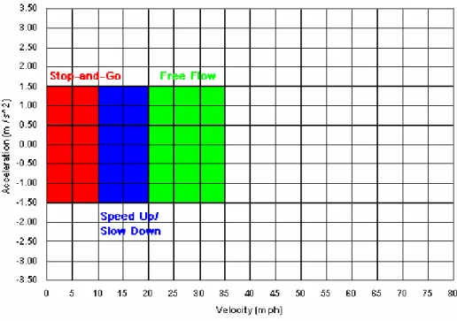
First of all, this thesis restricts reasonable driving situations in the area of [V: 0 ~ 80 mph, A: -3.5 ~ 3.5 m/s2] and then evenly divides this area into 224 grids (16× 14, see Figure 2-1) with the consideration of differentiability. For each grid, the corresponding vehicle performance will be measured by the average fuel consumption and emissions of all the driving situations in that grid.

-3.50 -3.00 -2.50 -2.00 -1.50 -1.00 -0.50 0.00 0.50 1.00 1.50 2.00 2.50 3.00 3.50 0 5 10 15 20 25 30 35 40 45 50 55 60 65 70 75 80 Velocity (m ph) Acc e ler at io n ( m / s ^ 2)

(27)

Secondly, in land transportation systems, the concept of “Level-of-Service” (LOS) divides the levels of traffic congestion into six grades (A~F, from the best to the worst) and then defines these grades with road types and vehicle speed [TRB, 2000]. Considering the similarity between operation patterns and traffic congestion, this thesis assumes that “Free Flow” is equivalent to “A~B” levels of traffic congestion, “Speed Up/Slow Down” is equivalent to “C-D” levels of traffic congestion, and “Stop-and-Go” is equivalent to “E~F” levels of traffic congestion. Further, according to existing research [EPA, 1997], this thesis also makes several reasonable assumptions for the range of vehicle acceleration in each level of traffic congestion. All these assumptions and the concept of LOS are summarized in Table 2-1.

Table 2-1: LOS and Basic Assumptions

Road Type Level-of-Service Operation Pattern Velocity (mph) Acceleration (m/s2)

A~B Free Flow 50~70 -1.0~1.0

C~D Speed Up/Slow Down 40~50 -1.5~1.5

Highway

E~F Stop-and-Go 0~40 -3.0~3.0

A~B Free Flow 30~45 -2.0~2.0

Suburban

E~F Stop-and-Go 0~15 -2.5~2.5

A~B Free Flow 20~35 -1.5~1.5

Urban

E~F Stop-and-Go 0~10 -1.5~1.5

Finally, Table 2-1 reveals the relationships between road types, operation patterns, vehicle velocity and acceleration. Through mapping these relationships into the V-A graph (see Figures 2-2 ~ 2-4), this thesis can connect the definition for driving situations with the definition for “driving segments”.

(28)

Figure 2-2: Driving Situations and “Driving Segments” (Highway)

(29)

Figure 2-4: Driving Situations and “Driving Segments” (Urban Street)

For example, Figure 2-5 shows three sample “driving segments” in the V-A graph (vehicle speed is taken as the average velocity instead of the velocity range to be more specific): DS-1 represents the segment of [vehicle speed: 2.5 mph; operation pattern: Stop-and-Go; road type: Highway], DS-2 represents the segment of [vehicle speed: 42.5 mph; operation pattern: Speed Up/Slow Down; road type: Highway], and DS-3 represents the segment of [vehicle speed: 52.5 mph; operation pattern: Free Flow; road type: Highway]. From Figure 2-5, it is obvious that the vehicle performance of DS-1 equals the average fuel consumption and emissions of all the driving situations in the twelve Red grids, the vehicle performance of DS-2 equals the average fuel consumption and emissions of all the driving situations in the six Blue grids, and the vehicle performance of DS-3 equals the average fuel consumption and emissions of all the driving situations in the four Green grids. These relationships between driving situations and “driving segments” provide the basis for this thesis to develop the “Driving Segments” vehicle performance matrices to quantify the impacts of worsening traffic.

(30)

Figure 2-5: Three Sample “Driving Segments” on Highway

2.3 Vehicle Simulation Tool

As discussed in Chapter 1, because of the lack of experimental data, the fuel consumption and emissions of all the driving situations need to be generated by vehicle simulation tools.

Through comparing several professional tools for vehicle simulation (see Table 2-2), this thesis selects ADVISOR 2004 as the data source for instantaneous vehicle characteristics [AVL, 2004; Markel et al., 2002; EPA, 2003; EPA, 2004; ANL, 2005]. Specifically, ADVISOR is designed for rapid analysis of the fuel consumption and emissions of conventional and advanced, light and heavy-duty vehicle models as well as hybrid electric and fuel cell vehicle models.

(31)

Table 2-2: Comparison for Vehicle Simulation Tools

Tool Developer Output Feature

ADVISOR 2004 NREL / AVL Fuel Consumption and Emissions Vehicle Cycle

MOBILE 6 EPA Emissions Vehicle Cycle

MOVES 2004 EPA Emissions Vehicle Cycle

GREET 1.6 ANL Fuel Consumption and Emissions Fuel Cycle

After defining “driving segments” and choosing simulation tool, this thesis is able to apply the three-step method described in Chapter 1 (see Figure 1-5) to develop the “Driving Segments” vehicle performance matrices:

First, this thesis will use ADVISOR 2004 to simulate the fuel consumption and emissions (gram per second) of different vehicle type under selected standard driving cycles. Considering the fact that driving cycles consist of series of data points representing the velocity and acceleration of a vehicle versus time, ADVISOR 2004 actually produces the fuel consumption and emissions of many possible driving situations.

Second, this thesis will categorize the fuel consumption and emissions of these possible driving situations (from driving cycles) into the 224 grids in the V-A graph. Further, the vehicle performance under each V-A grid (i.e. “V-A” vehicle performance matrices) can be generated by averaging the fuel consumption and emissions of all the driving situations in the same grid.

Third, according to the graphic definition for “driving segments” (see Figures 2-2 ~ 2-4), the vehicle performance under each “driving segment” (i.e. “Driving Segments” vehicle performance matrices, or “Velocity-Pattern” vehicle performance matrices) can finally be developed from the above “V-A” vehicle performance matrices.

(32)

Next, this thesis will discuss the simulation objects (vehicle classification and driving cycles) and the simulation results (“V-A” vehicle performance matrices and “Driving Segments” vehicle performance matrices) in detail.

2.4 Simulation Objects

2.4.1 Vehicle Classification

As analyzed in Chapter 1, this thesis will only study the impacts of worsening traffic on light-duty vehicles, which are normally divided into passenger cars and light trucks. In addition, considering the need to develop new vehicle technologies (Hybrid Vehicles, Electric Vehicles, Fuel Cell Vehicles, etc.), this thesis finally defines 13 types of light-duty vehicles as well as corresponding simulation parameters, such as maximum power, peak efficiency and vehicle/cargo mass (see Table 2-3).

Especially, for 10 types of conventional light-duty vehicles, the difference of vehicle performance caused by different transmissions (automatic and manual) will also be compared in this thesis.

2.4.2 Driving Cycles

As mentioned before, because driving cycle consists of series of data points representing the velocity and acceleration of a vehicle versus time, the simulation of fuel consumption and emissions under a standard driving cycle actually provides the vehicle performance of many possible driving situations. In order to get enough driving situations to further calculate the vehicle performance of “driving segments”, more than one driving cycle

(33)

must be considered.

Through comparing the distribution of data points (of each driving cycle) on the V-A graph with the definition of “driving segments” (see Figures 2-2 ~ 2-4), the thesis selects 7 out of 54 standard driving cycles from the database of ADVISOR 2004. These 7 representative driving cycles (ARB02, CSHVR, FTP, LA92, IDLING, INRETS, and OCC) are defined as below and their V-A distribution are shown in Figures 2-6 ~ 2-12.

y ARB02 (Air Resources Board No. 2): a driving cycle developed by the California Air Resources Board, including some city like driving and a period of highway cruising.

y CSHVR (City Suburban Heavy Vehicle Route): a chassis dynamometer test cycle for heavy-duty vehicles developed by the West Virginia University.

y FTP (Federal Test Procedure): a transient test cycle for cars and light trucks performed on a chassis dynamometer, including the simulations for an urban route with frequent stops, aggressive highway driving and the use of air conditioning units.

y LA92 (Los Angeles 92): 1992 test data from Los Angeles that consists of urban / highway mix and can be characterized by aggressive urban driving.

y IDLING: a chassis dynamometer test cycle only representing the idle status of vehicles.

y INRETS (Institut National de REcherche sur les Transports et leur Sécurité): a short urban driving cycle developed by the French national institute for transport and safety research.

y OCC (Orange County Cycle): a chassis dynamometer test cycle for transit buses developed by the West Virginia University.

(34)

The above definitions show that not all these 7 driving cycles are developed for light-duty vehicles. However, in order to get the vehicle performance under each “driving segment” (see Figures 2-2 ~ 2-4), this thesis only cares about the distribution of data points on the velocity-acceleration map and therefore it is reasonable to use those driving cycles for heavy-duty vehicles in this thesis.

2.5 Simulation Results

2.5.1 “Velocity-Acceleration” Vehicle Performance Matrices

With the above objects, ADVISOR 2004 needs to simulate the fuel consumption and emissions of 13 light-duty vehicle types under 7 representative driving cycles. In this thesis, all kinds of fuel consumption (gasoline, diesel, electricity and hydrogen) will be converted into gasoline equivalence on the basis of low heating value (LHV), and only the emissions of four major pollutants (CO2, HC, NOX and CO) will be considered.

For each vehicle type, 7 driving cycles totally provide 11232 data points (driving situations). In order to analyze so many driving situations, this thesis compiles a special C++ program (see Program A-2-1) to categorize these driving situations into the 224 V-A grids. After that, this program will automatically calculate the average fuel consumption and emissions of all the driving situations in the same grid, and these average fuel consumption and emissions constitute the (approximate) “V-A” vehicle performance matrices (see Table 2-4, the example of Two-seater Car with automatic transmission).

(35)

Table 2-3: Vehicle Classification and Simulation Parameters

Vehicle Classification No. Drivetrain Fuel Converter

MaxPower (kW) Peak Efficiency Transmission Mass/Cargo (kg)

Two-seater Car 1 Conventional IC-SI-Gasoline 41 0.34 Auto/Manual 984/136

Subcompact 2 Conventional IC-SI-Gasoline 63 0.34 Auto/Manual 1319/136

Compact 3 Conventional IC-SI-Gasoline 63 0.34 Auto/Manual 1466/136

Midsize 4 Conventional IC-SI-Gasoline 63 0.34 Auto/Manual 1541/136

Passenger

Cars Sedan

Large 5 Conventional IC-SI-Gasoline 63 0.34 Auto/Manual 1492/136

Small 6 Conventional IC-SI-Gasoline 102 0.29 Auto/Manual 1573/136

Pickup

Small 8 Conventional IC-SI-Gasoline 102 0.29 Auto/Manual 1970/136

Van

Conventional

Light

Trucks

SUV 10 Conventional IC-SI-Gasoline 144 0.34 Auto/Manual 1924/136

Hybrid: Prius (midsize) 11 Hybrid IC-SI-Gasoline 43 0.39 Auto=Manual 1332/136

EV 12 Electricity - 75 0.92 Auto=Manual 1144/136

New

Passenger

Cars

(36)

-3.50 -3.00 -2.50 -2.00 -1.50 -1.00 -0.50 0.00 0.50 1.00 1.50 2.00 2.50 3.00 3.50 0 5 10 15 20 25 30 35 40 45 50 55 60 65 70 75 80 Velocity (m ph) A cceler at io n ( m /s^ 2 ) -3.50 -3.00 -2.50 -2.00 -1.50 -1.00 -0.50 0.00 0.50 1.00 1.50 2.00 2.50 3.00 3.50 0 5 10 15 20 25 30 35 40 45 50 55 60 65 70 75 80 Velocity (m ph) A cceler at io n ( m /s^ 2 )

Figure 2-6: V-A Distribution for ARB02 Figure 2-7: V-A Distribution for CSHVR

-3.50 -3.00 -2.50 -2.00 -1.50 -1.00 -0.50 0.00 0.50 1.00 1.50 2.00 2.50 3.00 3.50 0 5 10 15 20 25 30 35 40 45 50 55 60 65 70 75 80 Velocity (m ph) A c c e le ra ti o n ( m /s ^ 2 ) -3.50 -3.00 -2.50 -2.00 -1.50 -1.00 -0.50 0.00 0.50 1.00 1.50 2.00 2.50 3.00 3.50 0 5 10 15 20 25 30 35 40 45 50 55 60 65 70 75 80 Velocity (m ph) A c c e le ra ti o n ( m /s ^ 2 )

Figure 2-8: V-A Distribution for FTP Figure 2-9: V-A Distribution for LA-92

-3.50 -3.00 -2.50 -2.00 -1.50 -1.00 -0.50 0.00 0.50 1.00 1.50 2.00 2.50 3.00 3.50 0 5 10 15 20 25 30 35 40 45 50 55 60 65 70 75 80 Velocity (m ph) A ccel er at io n ( m /s ^ 2 ) -3.50 -3.00 -2.50 -2.00 -1.50 -1.00 -0.50 0.00 0.50 1.00 1.50 2.00 2.50 3.00 3.50 0 5 10 15 20 25 30 35 40 45 50 55 60 65 70 75 80 Velocity (m ph) A ccel er at io n ( m /s ^ 2 )

(37)

-3.50 -3.00 -2.50 -2.00 -1.50 -1.00 -0.50 0.00 0.50 1.00 1.50 2.00 2.50 3.00 3.50 0 5 10 15 20 25 30 35 40 45 50 55 60 65 70 75 80 Velocity (m ph) A c c e le ra ti o n ( m /s ^ 2 )

Figure 2-12: V-A Distribution for OCC

Table 2-4: “V-A” Vehicle Performance Matrix for Two-seater Car (Automatic Transmission)

Velocity Accel Fuel CO2 HC NOX CO

(mph) (m/s^2) (g/s) (g/s) (g/s) (g/s) (g/s) [0, 5) [-3.5, -3.0) 0.119 0.371 0.000 0.000 0.000 [0, 5) [-3.0, -2.5) 0.125 0.388 0.000 0.000 0.000 [0, 5) [-2.5, -2.0) 0.123 0.385 0.000 0.000 0.000 [0, 5) [-2.0, -1.5) 0.127 0.390 0.000 0.000 0.001 [0, 5) [-1.5, -1.0) 0.130 0.397 0.000 0.000 0.003 [0, 5) [-1.0, -0.5) 0.140 0.424 0.001 0.000 0.004 [0, 5) [-0.5, 0.0) 0.200 0.599 0.002 0.001 0.007 [0, 5) [0.0, 0.5) 0.145 0.426 0.003 0.001 0.009 [0, 5) [0.5, 1.0) 0.308 0.925 0.003 0.002 0.010 [0, 5) [1.0, 1.5) 0.331 0.992 0.005 0.003 0.011 [0, 5) [1.5, 2.0) 0.367 1.072 0.007 0.004 0.024 [0, 5) [2.0, 2.5) 0.345 1.045 0.003 0.003 0.008 [0, 5) [2.5, 3.0) 0.358 1.101 0.001 0.001 0.002 [0, 5) [3.0, 3.5] 0.820 2.468 0.002 0.002 0.040 [5, 10) [-3.5, -3.0) 0.127 0.391 0.000 0.000 0.001 [5, 10) [-3.0, -2.5) 0.130 0.399 0.000 0.000 0.001 [5, 10) [-2.5, -2.0) 0.129 0.397 0.000 0.000 0.001 [5, 10) [-2.0, -1.5) 0.145 0.441 0.001 0.000 0.003 [5, 10) [-1.5, -1.0) 0.149 0.447 0.001 0.000 0.006 [5, 10) [-1.0, -0.5) 0.157 0.472 0.001 0.000 0.005 [5, 10) [-0.5, 0.0) 0.188 0.568 0.002 0.000 0.005 [5, 10) [0.0, 0.5) 0.303 0.908 0.002 0.002 0.013 [5, 10) [0.5, 1.0) 0.419 1.239 0.007 0.005 0.022 [5, 10) [1.0, 1.5) 0.600 1.774 0.006 0.006 0.038 [5, 10) [1.5, 2.0) 0.579 1.642 0.006 0.005 0.081 [5, 10) [2.0, 2.5) 0.705 2.143 0.002 0.002 0.018 [5, 10) [2.5, 3.0) 0.855 2.500 0.009 0.005 0.072 [5, 10) [3.0, 3.5] 1.108 3.241 0.010 0.005 0.097 …… …… …… …… …… …… …… [75, 80] [-3.5, -3.0) 0.290 0.912 0.004 0.002 0.000 [75, 80] [-3.0, -2.5) 0.090 0.293 0.000 0.000 0.000 [75, 80] [-2.5, -2.0) 0.188 0.580 0.001 0.000 0.000 [75, 80] [-2.0, -1.5) 0.470 1.436 0.001 0.000 0.008 [75, 80] [-1.5, -1.0) 0.950 2.874 0.002 0.001 0.034 [75, 80] [-1.0, -0.5) 1.358 4.114 0.003 0.002 0.045 [75, 80] [-0.5, 0.0) 1.751 5.300 0.003 0.004 0.060 [75, 80] [0.0, 0.5) 1.835 5.546 0.003 0.003 0.070 [75, 80] [0.5, 1.0) 1.591 4.801 0.003 0.003 0.065 [75, 80] [1.0, 1.5) 0.362 1.084 0.003 0.000 0.014 [75, 80] [1.5, 2.0) 3.369 10.137 0.004 0.003 0.163 [75, 80] [2.0, 2.5) 2.012 6.070 0.005 0.005 0.083 [75, 80] [2.5, 3.0) 1.889 5.904 0.000 0.000 0.000 [75, 80] [3.0, 3.5] 1.765 5.738 0.000 0.000 0.000

(38)

Especially, for a few grids into which no driving situation falls, their associated fuel consumption and emissions will be linearly interpolated or extrapolated from the vehicle performance of adjacent grids. Moreover, all these interpolations and extrapolations will be taken along both V axis and A axis and then be averaged to improve the accuracy.

2.5.2 “Driving Segments” Vehicle Performance Matrices

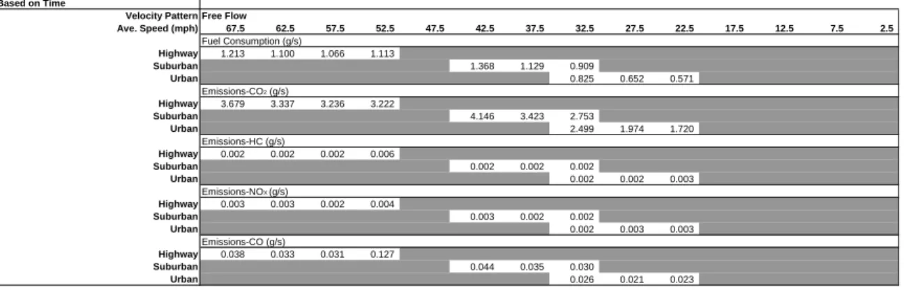
Combining the “V-A” vehicle performance matrices with the graphic definition of “driving segments” (see Figures 2-2 ~ 2-4), the average fuel consumption and emissions in each “driving segment” can be finally developed into the “Driving Segments” (or “Velocity-Pattern”) vehicle performance matrices. Table 2-5 gives the example of Two-seater Car with automatic transmission under the “Free Flow” pattern.

Table 2-5: “Driving Segments” Vehicle Performance Matrix for Two-seater Car (Automatic, Free Flow, Time)

Based on Time

Velocity Pattern Free Flow

Ave. Speed (mph) 67.5 62.5 57.5 52.5 47.5 42.5 37.5 32.5 27.5 22.5 17.5 12.5 7.5 2.5 Fuel Consumption (g/s) Highway 1.213 1.100 1.066 1.113 Suburban 1.368 1.129 0.909 Urban 0.825 0.652 0.571 Emissions-CO2 (g/s) Highway 3.679 3.337 3.236 3.222 Suburban 4.146 3.423 2.753 Urban 2.499 1.974 1.720 Emissions-HC (g/s) Highway 0.002 0.002 0.002 0.006 Suburban 0.002 0.002 0.002 Urban 0.002 0.002 0.003 Emissions-NOX (g/s) Highway 0.003 0.003 0.002 0.004 Suburban 0.003 0.002 0.002 Urban 0.002 0.003 0.003 Emissions-CO (g/s) Highway 0.038 0.033 0.031 0.127 Suburban 0.044 0.035 0.030 Urban 0.026 0.021 0.023

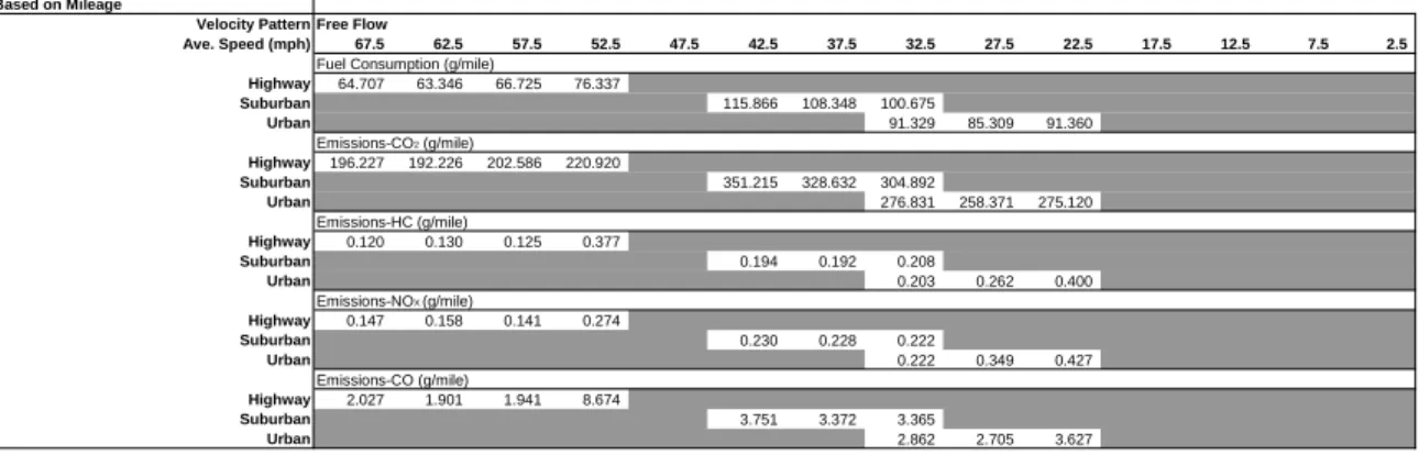
As pointed out before, the units for fuel consumption and emissions in Table 2-5 are “gram per second” because the definition of driving cycles (data points representing driving situations versus time) determines the output of ADVISOR 2004. Divided by the average vehicle speed for each segments, the units of vehicle performance can be easily changed into “gram per mile” (see Table 2-6), which may be more useful to analyze the energy and environmental impacts of worsening traffic in the next two chapters.

(39)

Table 2-6: “Driving Segments” Vehicle Performance Matrix for Two-seater Car (Automatic, Free Flow, Mileage)

Based on Mileage

Velocity Pattern Free Flow

Ave. Speed (mph) 67.5 62.5 57.5 52.5 47.5 42.5 37.5 32.5 27.5 22.5 17.5 12.5 7.5 2.5

Fuel Consumption (g/mile)

Highway 64.707 63.346 66.725 76.337 Suburban 115.866 108.348 100.675 Urban 91.329 85.309 91.360 Emissions-CO2 (g/mile) Highway 196.227 192.226 202.586 220.920 Suburban 351.215 328.632 304.892 Urban 276.831 258.371 275.120 Emissions-HC (g/mile) Highway 0.120 0.130 0.125 0.377 Suburban 0.194 0.192 0.208 Urban 0.203 0.262 0.400 Emissions-NOX (g/mile) Highway 0.147 0.158 0.141 0.274 Suburban 0.230 0.228 0.222 Urban 0.222 0.349 0.427 Emissions-CO (g/mile) Highway 2.027 1.901 1.941 8.674 Suburban 3.751 3.372 3.365 Urban 2.862 2.705 3.627

All the “Driving Segments” vehicle performance matrices for 13 light-duty vehicle types (both time-based and mileage-based) have been summarized in Tables A-2-1 ~ A-2-23 (see the Appendix).

2.6 Summary

This Chapter gives the detailed definition of “driving segments” and establishes the relationship between driving situations and “driving segments” on the V-A graph.

With the aid from ADVISOR 2004, this Chapter also develops the time-based and mileage-based “Driving Segments” vehicle performance matrices for 13 light-duty vehicle types, which provide the solid basis for analyzing the impacts of worsening traffic in the next two chapters.

(40)

(41)

CHAPTER 3: IMPACTS OF WORSENING TRAFFIC ON

INDIVIDUAL VEHICLES

3.1 Introduction

Mobile sources have been identified as major contributors to energy and environmental problems in the U.S. [EIA, 2005]. Thus, it is important that there be accurate fuel consumption and emissions inventories for mobile sources, especially for light-duty vehicles, which constitute the greatest proportion of the U.S. on-road vehicle fleet. However, the fuel consumption and emissions of light-duty vehicles are generally tested under standard driving cycles, which can not well describe the real-world driving patterns influenced by worsening traffic [Samuel et al., 2003].

With the “Driving Segments” (or “Velocity-Pattern”) matrices developed in Chapter 2, vehicle performance under any driving situations can be easily calculated. In other words, the “on-road” fuel consumption and emissions of light-duty vehicles can be quantified through specific “driving segments” stemming from real traffic situations. Further, the change of individual vehicle performance caused by worsening traffic can also be investigated.

For simplicity, this Chapter first analyzes individual vehicle performance on the basis of single commute with the “Velocity-Acceleration” vehicle performance matrices. After that, a rough traffic model is assumed to reflect the comprehensive effects of worsening traffic on all kinds of commutes. Through linking this traffic assumption and the “Driving Segments” vehicle performance matrices, the “on-road” fuel consumption and emissions

(42)

of 13 light-duty vehicle types as well as the impacts of worsening traffic on vehicle performance are examined.

3.2 Individual Vehicle and Single Commute

In order to study the individual vehicle performance over single commute, this Chapter defines a typical daily work commute from home to office and three sets of driving situations determined by traffic congestion on this commute. Through adjusting the proportion of different driving situation sets among annual driving trips, three scenarios for traffic change from 2005 to 2010 are also defined. Combining these commute and traffic definitions with the “Velocity-Acceleration” vehicle performance matrices, the annual fuel consumption and emissions of individual vehicle under different traffic scenarios can be calculated. For simplicity, the following assumptions have been made:

• Only four types of light-duty vehicle are considered here: Compact Sedan, Midsize Sedan, SUV, and Hybrid (Toyota Prius);

• Only light-duty vehicles with automatic transmission are considered;

• The impacts of technology development on vehicle performance are ignored during this five-year-long period (2005 ~ 2010).

3.2.1 Commute Description

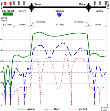
From home to office, the daily work commute consists of one urban section (side-street), two suburban sections (artery) and one highway section which are 18.6 miles totally in length. Traffic light, stop sign and highway ramp have also been included in this commute to best simulate the real traffic situations (see Figure 3-1).

(43)

The traffic situations on this commute can be roughly classified into three grades: “normal”, “busy” and “snarled”, which represent increasingly worse congestion levels. Based on several real cases, three sets of driving situations including velocity, acceleration and time duration under “normal”, “busy” and “snarled” traffic situations are defined in Table 3-1.

In addition, Figure 3-1 and Figure 3-2 graphically describe these three sets of driving situations from different views (velocity-distance and velocity-time).

Table 3-1: Three Sets of Driving Situations

SIDE-STREET ARTERY RAMP HIGHWAY RAMP ARTERY TOTAL

Run Idle Run Idle Run Idle Run Idle

DISTANCE (mile) 2.0 0.0 3.0 0.0 0.3 10.0 0.0 0.3 3.0 0.0 18.6 miles

NORMAL Velocity (mph) 35.0 0.0 45.0 0.0 55.0 65.0 0.0 55.0 45.0 0.0

Time (min) 3.4 1.0 4.0 0.0 0.3 9.2 0.0 0.3 4.0 0.0 22.3 minutes

Max Accel. (mph/s) 3.7 0.0 5.0 0.0 1.0 2.7 0.0 1.0 5.0 0.0

BUSY Velocity (mph) 20.0 0.0 30.0 0.0 40.0 50.0 0.0 40.0 30.0 0.0

Time (min) 6.0 2.0 6.0 1.0 0.5 12.0 0.0 0.5 6.0 1.0 34.9 minutes

Max Accel. (mph/s) 3.7 0.0 5.7 0.0 0.7 3.4 0.0 0.7 5.7 0.0

SNARLED Velocity (mph) 10.0 0.0 15.0 0.0 27.5 40.0 0.0 27.5 15.0 0.0

Time (min) 12.0 3.0 12.0 2.0 0.7 15.0 2.0 0.7 12.0 2.0 61.3 minutes

(44)

Figure 3-1: Driving Situation Description (Velocity-Distance)

(45)

3.2.2 Traffic Assumptions

This daily work commute only considers traveling from home to office, and therefore it is assumed that there are 240 trips on this commute per year, after deducting all the holidays. Further, according to practical experience, it is also assumed that in 2005, 70% of these 240 trips belong to “normal” traffic situation, 20% of these trips belong to “busy” traffic situation, and the remaining 10% of these trips fall into “snarled” traffic situation.

Based on the above two assumptions, this Chapter defines three scenarios for the traffic change from 2005 to 2010, namely, “same”, “bad” and “horrible” (see Table 3-2 and Figure 3-3). From “same” scenario to “horrible” scenario, it is obvious that the traffic situation in 2010 becomes worse, which is consistent with existing research on the trend of traffic congestion [TTI, 2005].

Table 3-2: Traffic Assumptions for 2005 and 2010

NORMAL BUSY SNARLED

percent trips percent trips percent trips

2005 70% 168 20% 48 10% 24 2010 Same 70% 168 20% 48 10% 24 Bad 50% 120 30% 72 20% 48 Horrible 30% 72 40% 96 30% 72 0 50 100 150 200 250 300

2005 2010 Sam e 2010 Bad 2010 Horrible

tr

ip

s /

year

Norm al Busy Snarled

(46)

3.2.3 Vehicle Performance Assessment

Combining the above three sets of driving situations and traffic assumptions with the “Velocity-Acceleration” vehicle performance matrices developed in Chapter 2, the “on-road” fuel consumption and emissions of four common light-duty vehicle types under different traffic scenarios can be quantified through the following two steps:

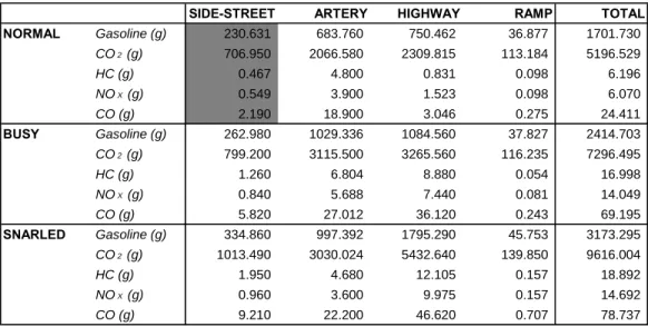
First, calculating the “per-trip” fuel consumption and emissions from the “Velocity-Acceleration” matrices and driving situation definitions. As discussed in Chapter 2, every common driving situation can be categorized into one of the 224 grids on the velocity-acceleration graph (velocity: 0 ~ 80 mph, acceleration: -3.5 ~ 3.5 m / s2, see Figure 3-4), and the “Velocity-Acceleration” matrices, which are measured in time units, give the average fuel consumption and emissions for all the driving situations in the same grid (see Table 3-3, the example of Compact Sedan). On the other hand, the driving situations and their time duration for “normal”, “busy” and “snarled” trips are described by the driving situation definitions (see Table 3-1 and Figures 3-1, 3-2). Therefore, the “per-trip” fuel consumption and emissions of individual vehicle (see Table 3-4, the example of Compact Sedan) can be generated by multiplying the vehicle performance in “Velocity-Acceleration” matrices and the corresponding time duration in driving situation definitions.

For instance, according to the definition for the “normal” trip in Figures 3-1 and 3-2, the driving situations on the side-street can be represented with the grey areas in Figure 3-4. Furthermore, the grey values in Table 3-3 and Table 3-1 respectively provide the vehicle performance and time durations of these driving situations. Multiplying the grey values in these two tables, the fuel consumption and emissions on the side-street during the “normal” trip can be calculated and then summarized in the grey area of Table 3-4.

(47)

Figure 3-4: Velocity-Acceleration Graph for Vehicle Performance

Table 3-3: Velocity-Acceleration Matrices for Compact Sedan

Velocity Accel Gasoline CO2 HC NOX CO (mph) (m/s^2) (g/s) (g/s) (g/s) (g/s) (g/s) [0, 5) [-3.50, -3.00) 0.187 0.582 0.000 0.000 0.000 [0, 5) [-3.00, -2.50) 0.196 0.605 0.000 0.000 0.000 [0, 5) [-2.50, -2.00) 0.192 0.598 0.000 0.000 0.000 [0, 5) [-2.00, -1.50) 0.198 0.608 0.000 0.000 0.001 [0, 5) [-1.50, -1.00) 0.203 0.618 0.000 0.000 0.004 [0, 5) [-1.00, -0.50) 0.220 0.668 0.001 0.000 0.005 [0, 5) [-0.50, 0.00) 0.285 0.862 0.001 0.000 0.008 [0, 5) [0.00, 0.50) 0.229 0.687 0.002 0.000 0.009 [0, 5) [0.50, 1.00) 0.383 1.160 0.002 0.001 0.010 [0, 5) [1.00, 1.50) 0.423 1.276 0.003 0.001 0.013 [0, 5) [1.50, 2.00) 0.478 1.432 0.005 0.002 0.019 [0, 5) [2.00, 2.50) 0.442 1.344 0.002 0.001 0.010 [0, 5) [2.50, 3.00) 0.464 1.429 0.001 0.000 0.002 [0, 5) [3.00, 3.50) 0.487 1.514 0.000 0.000 0.000 … … … … [30, 35) [-3.50, -3.00) 0.208 0.637 0.000 0.000 0.002 [30, 35) [-3.00, -2.50) 0.194 0.595 0.000 0.000 0.001 [30, 35) [-2.50, -2.00) 0.199 0.611 0.000 0.000 0.001 [30, 35) [-2.00, -1.50) 0.199 0.606 0.000 0.000 0.003 [30, 35) [-1.50, -1.00) 0.206 0.631 0.000 0.000 0.002 [30, 35) [-1.00, -0.50) 0.286 0.877 0.000 0.000 0.002 [30, 35) [-0.50, 0.00) 0.453 1.384 0.001 0.001 0.006 [30, 35) [0.00, 0.50) 0.928 2.840 0.003 0.003 0.011 [30, 35) [0.50, 1.00) 1.762 5.411 0.003 0.005 0.012 [30, 35) [1.00, 1.50) 2.642 8.121 0.004 0.007 0.016 [30, 35) [1.50, 2.00) 3.795 11.427 0.033 0.026 0.122 [30, 35) [2.00, 2.50) 5.300 16.051 0.034 0.031 0.133 [30, 35) [2.50, 3.00) 4.931 14.863 0.042 0.032 0.149 [30, 35) [3.00, 3.50) 4.563 13.675 0.049 0.034 0.165 … … … … [75, 80) [3.00, 3.50) 2.091 7.060 0.000 0.000 0.000

(48)

Table 3-4: “Per-Trip” Fuel Consumption and Emissions of Compact Sedan

SIDE-STREET ARTERY HIGHWAY RAMP TOTAL

NORMAL Gasoline (g) 230.631 683.760 750.462 36.877 1701.730 CO2 (g) 706.950 2066.580 2309.815 113.184 5196.529 HC (g) 0.467 4.800 0.831 0.098 6.196 NOX (g) 0.549 3.900 1.523 0.098 6.070 CO (g) 2.190 18.900 3.046 0.275 24.411 BUSY Gasoline (g) 262.980 1029.336 1084.560 37.827 2414.703 CO2 (g) 799.200 3115.500 3265.560 116.235 7296.495 HC (g) 1.260 6.804 8.880 0.054 16.998 NOX (g) 0.840 5.688 7.440 0.081 14.049 CO (g) 5.820 27.012 36.120 0.243 69.195 SNARLED Gasoline (g) 334.860 997.392 1795.290 45.753 3173.295 CO2 (g) 1013.490 3030.024 5432.640 139.850 9616.004 HC (g) 1.950 4.680 12.105 0.157 18.892 NOX (g) 0.960 3.600 9.975 0.157 14.692 CO (g) 9.210 22.200 46.620 0.707 78.737

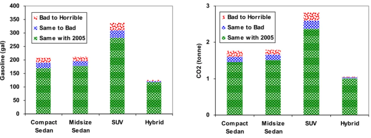
Second, calculating the annual fuel consumption and emissions from the “per-trip” vehicle performance and traffic assumptions. Once the “per-trip” fuel consumption and emissions of individual vehicle are calculated out, the annual fuel consumption and emissions can be obtained by aggregating the products of the “per-trip” vehicle performance (see Table 3-4) and the corresponding trip amount defined in the traffic assumptions (see Table 3-2). Table 3-5 gives the calculation results for Compact Sedan.

Table 3-5: Annual Morning Commute Fuel Consumption and Emissions of Compact Sedan

2010 SCENARIOS ∆q

Same Bad Horrible

Gasoline (tonne/year) 0.478 0.530 0.583 0.052

CO2 (tonne/year) 1.454 1.610 1.767 0.156

HC (kg/year) 2.310 2.874 3.438 0.564

NOX (kg/year) 2.047 2.445 2.844 0.398

CO (kg/year) 9.312 11.691 14.069 2.379

Through the above two steps, the annual vehicle performance for each of these four light-duty vehicle types can be quantified (see Figures 3-5 ~ 3-14).