HAL Id: hal-00302571
https://hal.archives-ouvertes.fr/hal-00302571
Submitted on 15 Mar 2005
HAL is a multi-disciplinary open access
archive for the deposit and dissemination of
sci-entific research documents, whether they are
pub-lished or not. The documents may come from
teaching and research institutions in France or
abroad, or from public or private research centers.
L’archive ouverte pluridisciplinaire HAL, est
destinée au dépôt et à la diffusion de documents
scientifiques de niveau recherche, publiés ou non,
émanant des établissements d’enseignement et de
recherche français ou étrangers, des laboratoires
publics ou privés.
automata and information theory
A. Jiménez, A. M. Posadas, J. M. Marfil
To cite this version:
A. Jiménez, A. M. Posadas, J. M. Marfil. A probabilistic seismic hazard model based on cellular
automata and information theory. Nonlinear Processes in Geophysics, European Geosciences Union
(EGU), 2005, 12 (3), pp.381-396. �hal-00302571�
Nonlinear Processes in Geophysics, 12, 1–16, 2005 SRef-ID: 1607-7946/npg/2005-12-1
European Geosciences Union
© 2005 Author(s). This work is licensed under a Creative Commons License.
Nonlinear Processes
in Geophysics
A probabilistic seismic hazard model based on cellular automata
and information theory
A. Jim´enez1, 2, A. M. Posadas1, 2, 3, and J. M. Marfil1, 2
1Department of Applied Physics, University of Almer´ıa, Spain
2Andalusian Institute of Geophysics and Seismic Disasters Prevention, Spain 3“Henri Poincar´e” Chair of Complex Systems, University of La Havana, Cuba
Received: 25 November 2004 – Accepted: 12 January 2005 – Published:
Abstract. We try to obtain a spatio-temporal model of earth-quakes occurrence based on Information Theory and Cellular Automata (CA). The CA supply useful models for many in-vestigations in natural sciences; here, it have been used to es-tablish temporal relations between the seismic events occur-ring in neighbouoccur-ring parts of the crust. The catalogue used is divided into time intervals and the region into cells, which are declared active or inactive by means of a certain energy release criterion (four criteria have been tested). A pattern of active and inactive cells which evolves over time is given. A stochastic CA is constructed with the patterns to simulate their spatio-temporal evolution. The interaction between the cells is represented by the neighbourhood (2-D and 3-D mod-els have been tried). The best model is chosen by maximiz-ing the mutual information between the past and the future states. Finally, a Probabilistic Seismic Hazard Map is drawn up for the different energy releases. The method has been ap-plied to the Iberian Peninsula catalogue from 1970 to 2001. For 2-D, the best neighbourhood has been the Moore’s one of radius 1; the von Neumann’s 3-D also gives hazard maps and takes into account the depth of the events. Gutenberg-Richter’s law and Hurst’s analysis have been obtained for the data as a test of the catalogue. Our results are consistent with previous studies both of seismic hazard and stress conditions in the zone, and with the seismicity occurred after 2001.
1 Introduction
The origin of modern science is based on the idea of reduc-tionism. Since Democritus and Epicure, the macroscopic be-haviour of matter has been explained in terms of its final con-stituents. This first approximation is a natural way to start the difficult challenge of understanding nature. Indeed it has been successful: with such a scheme we have understood the structure of the matter by using simple elements as atoms and
Correspondence to: A. Jim´enez
molecules. The knowledge of atoms and their structure has explained important properties of solids, fluids and plasmas, and has been used to transform the world in what we know today. However, with this reductionistic scheme one cannot explain why a metal is so different from a cell, as both of them are built with the same atoms. Other frameworks are needed, that of complex and/or non linear systems, where the whole is more than the sum of its parts. Until recently, the paradigm of science was to consider that simple systems (with a few variables) behaved in a simple manner (ordered), and that complex systems (with many variables) behaved in a complex manner (disordered, at random). However, it has been discovered that simple nonlinear systems can behave in a chaotic form. This implies that if one observes a disordered and complex behaviour in a system, it could effectively be a complex system or it could be a simple one, whose dynam-ics is chaotic. On the other hand, one could have a complex system with simple dynamics, due to a nonlinear synchro-nization and/or auto-orgasynchro-nization.
Even if the relation between the low-dimensional and the spatially-extended systems is too close, the former has a fun-damentally different property, and this is the formation of patterns. Spatially-extended dynamical systems in general are described by state spaces of infinite dimensionality. If, however, some emergent pattern or regularity in the config-uration of a system can be found, this pattern can be used to reduce the evolution of the system to some effectively low-dimensional, and therefore easier, dynamics. Discovery and identification of emergent patterns is therefore a crucial first step in the analysis of a system. If no such patterns can be found, the analysis must fall back on an approximate stochas-tic model of the evolution, although even that depends for its success on some statistical regularity in the behaviour (Han-son, 1993). Complex systems are not predictable with ab-solute precision; however, after a coarse-graining (on not too detailed a scale) a system becomes predictable (Keilis-Borok, 2003).
A spatially-extended system can be modeled by using “Cellular Automata” (CA), a simple class of
Neighborhood Rules
If 2 neighbors or more are If less than 2 neighbors are If 3 neighbors or more are If less than 3 neighbors are Lattice
Fig. 1. Elements of Cellular Automata.
idealized-discrete systems, which evolve in discrete space and time, and whose states are discrete too (Adamatzky, 1994). Each site value is updated according to rules that specify their values in terms of the values of neighbouring sites. In spite of its extreme simplicity, CA exhibit a wide range of behaviour (Wolfram, 1983): stationary uniform states, periodic ones in time and space, spatially disordered states, with turbulent behaviour, or in continuous evolution. For these reasons CA has been studied extensively in natural sciences, mathematics, and computer science.
Earthquakes have been represented in terms of discrete, spatially-extended systems, being each part of the crust in-teracting with its neighbouring parts; this approach repro-duces the same characteristics of self-affinity and power laws as earthquakes show (Burridge and Knopoff, 1967; Otsuka, 1972; Bak et al., 1988; Bak and Tang, 1989; Carlson and Langer, 1989a, b; Nakanishi, 1990, 1991; Barriere and Tur-cotte, 1991; Olami et al., 1992; Christensen and Olami, 1992).
The discrete approach has been also used by Hirata and Imoto (1997), Posadas et al. (2000), Posadas et al. (2002), Gonz´alez (2002) and Jim´enez et al. (2004) for characterizing the evolution of the seismicity in a region, and for providing maps (Probabilistic Seismic Hazard Maps) where the level of the future seismic activity is predicted in a probabilistic way. In the present paper this seismic hazard model is developed, taking into account the methods and tools of these authors. First, some basic concepts about CA as well as important results of the Information Theory will be presented. Next, the seismic hazard model will be exposed and applied to a particular region: the Iberian Peninsula. Finally, the main results and conclusions will be summarized.
2 Cellular automata
CA supply useful models for many investigations; in partic-ular, they represent a natural way of studying the evolution of large physical systems (Toffoli and Margolus, 1987). They are simple mathematical idealizations of natural systems, and consist of a lattice of discrete identical sites, each site taking on a finite set of integer values; values which evolve in dis-crete time steps according to rules that specify the value of each site in terms of the values of neighbouring sites. CA may thus be considered as discrete idealizations of the
par-tial differenpar-tial equations used to describe natural systems. Their discrete nature also allows an important analogy with digital computers: CA may be viewed as parallel-processing computers of simple construction (Wolfram, 1983).
A formal definition of CA is as follows (Delorme, 1998): a d-dimensional Cellular Automata (or d-CA), is a 4-uplet (Zd, S, n, δ), where Zd is a regular lattice (the elements of
Zd are called cells, or c), S is a finite set, the elements of which are the states of c; n is a finite ordered subset (with
m elements) of Zd, called the neighbourhood of c, and δ (Sm+1→S)is the local transition function or local rule of c (since the rules are homogeneous, δ is the same for the whole lattice).
In the construction of a CA to simulate a specific problem, many choices have to be made. Firstly, the available set of states for each cell (the S set); for simplicity, only two states are usually chosen, active or inactive (represented by black and white, respectively, Fig. 1). However, there are other CA with intermediate states between these two. A reason for preferring small state sets is that only when there are few states is it possible to specify the CA rules explicitly and store them in a table, which is important for simulation. A reason for using large numbers of states could be that these CA can better approximate a continuous system.
Another choice is the selection of a specific lattice geome-try (Zdgeometry, given by the cell geometry). The definition of CA requires the lattice to be regular. For one-dimensional automata, there is only one possibility: a linear array of cells. For two dimensions, three cell geometries can be selected: triangular, square and hexagonal. The first has the advantage of having a small number of nearest neighbours; but, it is difficult to represent or visualize (as it is the hexagonal one). So, the square geometry is the most commonly used, and, if a higher isotropy would be needed, the hexagonal one is the best. There are many possibilities in three dimensions; the easiest to handle and represent is the cubic one.
The lattice (Zd)is defined as infinite in all dimensions. For considerations of computability and complexity, this is reasonable and necessary; but, of course, it is impossi-ble to simulate a truly infinite lattice on a computer (un-less the active region always remains finite). Therefore it is necessary to prescribe some boundary conditions; in gen-eral, there are three kinds of them: periodic, reflective and fixed value. All three conditions can be combined, so that
A. Jim´enez et al.: A probabilistic seismic hazard model based on cellular automata and information theory 3
(a) (b) (c) (d) (e) (f) (g)
Fig. 2. Neighbourhoods, from left to right, the von Neumann’s with radii 1 and 2, that of Moore, of Smith and two of Cole, all in 2-D; and von Neumann’s neighbourhood radius 1 in 3-D.
different boundaries can have different conditions. Not only the boundary conditions have to be specified, but also the ini-tial conditions. They can be very special (constructed from data, for example), or they can be generated randomly.
Next, a neighbourhood (n) must be selected. The neigh-bourhood of a cell c (including the cell itself or not, accord-ing to the convention used) is the set of cells which will determine the evolution of c. It is finite and geometrically uniform. A neighbourhood can be any ordered finite set, but some special ones are mainly considered. Classic neigh-bourhoods are those of von Neumann and Moore. They are known as the “nearest neighbours neighbourhoods”, and de-fined according to the usual norms kzk1, kzk∞,and the as-sociated distances. More precisely, if z=(z1, ..., zd):
kzk1=Xd
i=1|zi|
kzk∞=Max {|zi| / i ∈ {1, ..., d}} with d1and d∞their associated distances.
This gives for the von Neumann’s neighbourhood:
nV N(z) = {x/x ∈ Zdy d1(z, x) ≤1} with a given order,
and for the Moore’s neighbourhood:
nM(z) = {x/x ∈ Zdy d∞(z, x) ≤1} with a given order. Other interesting neighbourhoods appear in literature (Weimar, 1998; Delorme, 1998) and some of them are repre-sented in Fig. 2. Together with a modification of the rules, the extension of the neighbourhood sometimes leads to a much better isotropy, and is therefore often used when natural phe-nomena have to be modelled. Note that a large neighbour-hood is usually very inefficient to simulate.
The most important aspect of a CA is the transition rule or transition function, δ. It depends on: the lattice geometry, the neighbourhood, and the state set. Even though the transi-tion rule most directly determines the evolutransi-tion, it is in many cases not possible to predict the evolution of a CA other than by explicitly simulating it. The transition function can be expressed in many different ways, being the most direct to write down the outcome for each possible configuration of states in the neighbourhood. Further simplification can of-ten be achieved by grouping states together according to the symmetries of the lattice. Also, they can be implicit, in that the detailed rule has to be evaluated from some formula. In classical Cellular Automata Theory a rule is called totalistic
if it only depends on the sum of the states of all cells in the neighbourhood. It is called outer totalistic if it also depends on the state of the cell to be updated. Another classification is to distinguish between deterministic or probabilistic rules. In the first case, the transition rule is a function which has ex-actly one result for each neighbourhood configuration. This corresponds to a Markov chain. However, probabilistic rules provide one or more possible states with associated proba-bilities, whose sum must be one for each input configuration (Weimar, 1998). In this case a model which is equivalent to a hidden Markov chain is obtained (Upper, 1997). Other classes are the so-called fuzzy CA, the hierarchical ones, or the exotic CA (Adamatzky, 1994).
3 Information theory
Information Theory confronts the problem of constructing models from experimental data series. These models are used to make predictions, but the underlying dynamics is unknown (or known but with a high dimensionality and thus incomputable). The limits of the predictive ability im-ply a loss of information, and motive the use of the for-malism and concepts of “Information Theory”. This the-ory, widely developed by Shannon (1948) and Shannon and Weaver (1949), often provides a natural and satisfactory framework for studying the predictability. Shannon studied the basic problem in sending and receiving messages, and realized that it was a statistical one. If messages are com-posed of an alphabet X with n symbols having the transmis-sion probabilities (p1,. . . , pn), the amount of information in a message is defined as:
H (X) = −K
n
X
i=1
pilog pi, (1)
where K is a positive units-dependent constant. Shannon ar-rived at this expression through arguments of common sense and consistency, along with requirements of continuity and additivity. Because information is often transmitted in strings of binary digits, it is conventional in Communication Theory to take the logarithm to the base 2 and measure H in “bits”. Thus, H quantifies the average information per symbol of in-put, measured in bits. Later, Jaynes (1957a, b) made a rigor-ous connection between Information Theory and the Physics. Whereas Shannon envisioned the set {pi}as given in Com-munication Theory, Jaynes turned the interpretation around
Fig. 3. Driscretization process at each interval of time.
to utilize available information to determine the probabili-ties.
The problem here is describing and quantifying the pre-dictability of a stream of numbers obtained from repeated measurements of a physical system. Shannon restricted his discussion to the transmission of information from a trans-mitter to a receiver through a channel, each with known sta-tistical properties: p(x) describing the distribution of possi-ble transmitted messages x∈X, p(y) the distribution of pos-sible received messages y∈Y , and the properties of the chan-nel connecting the two distributions is contained in the con-ditional distribution p(x|y), the probability of receiving mes-sage y given that mesmes-sage x was transmitted. A dynamical system communicates some information, but not necessary all, about its past state into the future; the conditional dis-tribution describes the causal connection between past and future, given by the system dynamics. Then, the problem of prediction, formally at least, becomes simple: given p(x) and p(x|y), compute p(y).
The amount of information that a random variable X con-tains about other random variable Y can be expressed by the “mutual information”. To explain its meaning, it is neces-sary first to define the Kullback-Leibler’s distance D(p||p0), also called relative entropy, which represents the distance be-tween two probability distribution functions, p and p0, of the same variable (Cover and Thomas, 1991):
D(p||p0) =Xplog2 p
p0 (2)
This distance can be interpreted as a measure of the impre-cision made by assuming a distribution p0when the true dis-tribution is p. With this quantity the mutual information, µI, is then defined as the relative entropy between the joint prob-ability distribution p(x, y) and the distribution given by the marginal probabilities p(x) and p(y) (Fraser and Swinney, 1986): µI(X; Y ) = n X i=1 m X j =1 p(xi, yj)log2 p(xi, yj) p(xi)p(yj) (3)
Note that when X and Y are independent, p(x, y)=p(x)p(y) (definition of independence), µI(X; Y )=0. This makes sense: if they are independent random variables, then Y will not tell us anything about X.
If X represents the seismicity of a region at a certain time and Y the seismicity at the same place but at a next interval of time, they will be related; the mutual information between them is an appropriate measure of how independent they are.
But this measurement depends on the time intervals consid-ered, as well as the way the areas which interact are defined, so that they establish a reasonable simplification of the real seismicity.
4 The method 4.1 The model
There is sustantial evidence of complex dynamics in the Earth’s crust. Following the “Tectonic Plates” theory, ad-vanced by Wegener (1912), the lithosphere is composed by a network of blocks (plates) which float over a viscous zone (asthenosphere) and interact between themselves. There are three main plate tectonic environments: extensional, trans-form, and compressional. Plate boundaries in different lo-calities are subject to different inter-plate stresses, produc-ing several types of earthquakes. The system lithosphere-asthenosphere, with the different plate interactions, forms a dynamical system of non linear, coupled equations, which consist in both internal plate equations (stresses, deforma-tions, ruptures, etc.) and relative plate movements. Such a system presents an extremely complex behaviour, although the equations are deterministic, because of their non lin-earity and coupling. This leads to a chaotic and/or com-plex approach to the seismologic studies, as in Crutchfield et al. (1986), Keilis-Borok (1990), Sotolongo et al. (2000) for example, or to consider the crust as blocks which interact (Burridge and Knopoff, 1967; Carlson and Langer, 1989a, b; Rundle et al., 1996).
Here we deal with a discrete representation of the seis-mic region, where each site is interacting with its neighbour-ing sites; the model is a CA, and it simulates the spatio-temporal evolution of the different seismic patterns obtained from the discretization process. More precisely, the model is a stochastic CA outer totalistic, whose boundary condi-tions are fixed (inactive edges) and whose initial condicondi-tions are given by the data. The class of CA chosen is the stochas-tic one because there are only two available states, and it is a generalization of a deterministic CA.
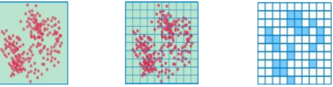
The seismic model proposed has four basic elements: a coarse-graining of the data, both spatially (the lattice is con-structed) and temporally; an activation criterion for the cell, that will lead to a simplification of the seismicity by assign-ing one of the two available values for each cell, active or inactive (the S set), and that will provide the seismic pat-tern, or lattice configuration, for each time; the template or neighbourhood, n, (2-D or 3-D) that determines how the cells interact; finally, the transition function, δ, which best repro-duces the pattern series.
The first two elements cited before, which lead to the pattern construction, are made by following the proposal of Hirata and Imoto (1997), Posadas et al. (2000, 2002), Gonz´alez (2002) and Jim´enez (2004): the seismic catalogue is divided into n0time intervals of length τ ; a coarse-graining is carried out for each τ , by dividing the region into Ndcells,
A. Jim´enez et al.: A probabilistic seismic hazard model based on cellular automata and information theory 5
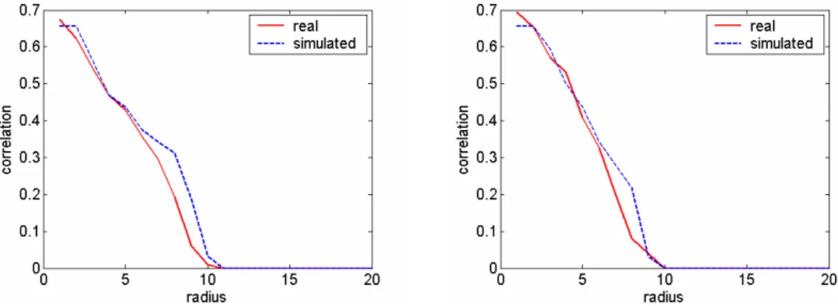
Fig. 4. Correlation functions of the simulations made for the 2-D von Neumann’s neighbourhood of radius 1 with the α1 criterion and the abridged catalogue. The Hamming distances are 12 and 9, respectively.
with N being the number of bins, or number of cells in one spatial dimension, and d the selected dimension; a state (ac-tive or inac(ac-tive) is assigned in function of a determined acti-vation criterion α.
The activation criterion homogenizes the information con-tained in each cell at each interval of time, and determines the pattern series to be fitted. In the works previously cited, a cell is declared active in a time interval τ if the number of events in that cell is greater than or equal to the average of the whole region at that interval. However, four different activity criteria have been here evaluated to give an adequate importance to the areas with less number of events, but with high magnitudes. A cell will be considered active if:
α1) the accumulated energy of the events at a time interval
τi is greater than or equal to the average of the whole region at the same interval;
α2) the accumulated energy is greater than or equal to a threshold energy;
α3) the maximum magnitude is greater than or equal to a threshold magnitude;
α4) the accumulated energy of the events until a time inter-val τiis greater than or equal to the average of the whole region.
The data set has been then translated to a CA representa-tion, where time, space and states are discrete (Fig. 3). The
α1 and α4 criteria provide an approach of the places where the maximum activity is foreseen. More precisely, the α4 cri-terion would be similar to the macroseismic studies, where the seismic hazard is evaluated from the whole catalogue in a zone. The α2 and α3 criteria mark the areas where cer-tain energy is expected to be surpassed (accumulated or peak energy).
The problem of obtaining the transition rules is an inverse one: given a pattern series, the δ function which best fits them has to be found. For each neighbourhood configuration there is a certain probability for each cell of being active or
inactive in the future (Jim´enez et al., 2004); two neighbour-hood configurations are considered equivalent if they have the same number of active neighbouring cells. The real prob-ability distributions can be obtained directly from the data, by using the Laplace probability concept (p(x)=favorable cases/possible cases). Thus, the CA rules are the dynami-cal model of the system, and characterize its spatio-temporal evolution.
Since there is no a priori knowledge of the best neighbour-hood to be used in the particular case of the seismic activ-ity, some of them have been tried: those denoted as “nearest neighbours neighbourhoods”, in 2-D (von Neumann’s radius 1, and Moore’s) and 3-D (von Neumann’s), and those of in-teraction at a longer distance (von Neumann’s radius 2, in 2-D).
Having fixed the activation criterion and the neighbour-hood, the δ function depends on the number of time intervals,
n0, and the number of cell, Nd. For choosing the best config-uration of both of them, it is necessary to use the results of the Information Theory. The mutual information is the function which measures the dependence between two variables, and its maximization gives the maximum dependence between these two variables. In this work, it is made by a grid-search in n0and N . As an example, for the von Neumann’s neigh-bourhood of radius 1 in 2-D, the mutual information can be expressed as: µI = 1 X i=0 1 X j =0 4 X k=0
p(i; j, k)log2 p(i; j, k)
p(i)p(j, k) (4)
being p(i; j, k) the joint probability of past and future states, and p(i)p(j, k) a distribution of independent states; (i) rep-resents the central cell in the future, and (j, k) the central and neighbouring cells in the past. For the Moore’s neigh-bourhood, the k index is extended to 8, which is the maxi-mum number of neighbouring cells. Once having the n0and
N which maximize µI, the stochastic CA rules are calcu-lated from the histograms of occurrence for each transition. Finally, this function is applied to the last real pattern for
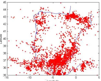
Fig. 5. Epicenter distribution of the earthquakes occurred in the Iberian Peninsula between 1970 and 2001.
constructing a Probabilistic Seismic Hazard Map for each en-ergy level (or magnitude) at the next τ in the future.
4.2 Simulations and tests
The pattern recognition technique previously exposed needs, to be complete, to include some tests which will inform about its fitness and will quantify the error levels in the method. These tests are used here for the first time in this kind of analysis, and are based on the simulation of the patterns and their comparison with the real ones. First, it is necessary to obtain the simulated patterns from the previous ones, and then to compare them with those that actually occurred. To generate the simulated patterns at t +τ from the real ones at time t , the CA rules of the model chosen have to be applied, and an activation probability is obtained for each cell. Then, the cells have to be declared active or inactive regarding these probabilities. One possibility for deciding the value of the threshold probability is to simulate the patterns for several densities of active cells, and the nearest value to the real one is chosen as the cutting probability (Posadas et al., 2000).
Once the real and simulated patterns for each time are obtained, some mathematical tools are needed to compare them. Those selected here are the correlation function (Vic-sek, 1992) and the Hamming distance. The first represents the probability of finding two points in the same sphere of radius r, by measuring the number of points x that are con-tained in a sphere of radius r centered at the point y (Grass-berger and Proccacia, 1983). The comparison between the real and simulated correlation functions informs about the similarity of both patterns. The Hamming distance is a com-mon way to compare two bit patterns, and it is defined as the number of bits different in the two patterns (Ryan and Frater, 2002). More generally, if two ordered lists of items are compared, the Hamming distance is the number of items that do not identically agree. This distance is applicable to
encoded information, and is a particularly simple metric of comparison. A complete study about tests and simulations was carried out for all the cases; as an example, the cor-relation functions of the simulation made for the 2-D von Neumann’s neighbourhood with the α1 criterion are shown (Fig. 4).
5 Data
The crustal deformation in the Iberian Peninsula, northwest-ern Africa and the adjacent offshore areas is controlled by the Africa-Eurasia plate collision and extensional processes in the western Mediterranean Basin and Alboran Sea. The regional seismicity is characterized by a diffuse geographi-cal distribution and from low to moderate magnitudes. Only in the Atlantic Ocean and northern of Algeria, seismic-ity appears to be focused around a linear plate boundary, and moderate to large earthquakes occur with a certain fre-quency. Earthquakes are rarely exceeding magnitude 5.0 on the Iberian Peninsula, northern Morocco, the westernmost Mediterranean Sea and the Atlantic Ocean south of Portugal (Stich et al., 2003).
The data used here has been recorded by the Geographic National Institute, which runs the National Seismic Network with 42 stations, 35 of them of short period, connected in real time with the Reception Centre of Seismic Data in Madrid. The catalogue, with more than 10 000 earthquakes in the re-gion between 35◦north and 45◦north latitude and between 15◦west and 5◦east longitude, contains all the seismic data in the Iberian Peninsula and northwestern Africa collected in the period 1970–2001 (Fig. 5). Their depths range from 0 to 146 km, and the magnitudes are between 1.0 and 6.5 (mb). The averaged error in the hypocentral localization at the di-rections X, Y and Z are ±5 km, ±5 km and ±10 km, respec-tively, for the data recorded until 1985, and ±1 km, ±1 km and ±2 km for those acquired since then.
Two tests have been made, to describe the nature of the data series (Gutenberg-Richter’s law) and their predictability (Hurst’s exponent). In first place, the frequency-magnitude distribution of earthquakes is expressed by the Gutenberg-Richter’s relation (Richter, 1958):
log s = a − bM, (5)
where sis the number of shocks of magnitude M or greater, a and b are constants. This relationship shows that the number of earthquakes declines logarithmically with the increase in magnitude. The extent of this decline is expressed by the b-value which is normally close to 1.0 (Mogi, 1985). Studies of Mogi (1963) and Scholz (1968) reveal that the b-value depends on the percentage of the rate of the existing stress to the final breaking stress within the fault. Also it depends on the mechanical heterogeneity of the rock and increases with the increase in heterogeneity. The high values of b are considered as a result of the low stresses in the zone, so that small earthquakes rather than large ones are more likely to
A. Jim´enez et al.: A probabilistic seismic hazard model based on cellular automata and information theory 7 occur. The expression of the Gutenberg-Richter’s law for the
used data set is:
log s (m) = (6.45 ± 0.08) − (0.982 ± 0.018) m (6) with a correlation coefficient of 0.985. The b-value can be interpreted as the result of a region where the stresses are relatively low. However, the seismicity can better be charac-terized with the value of a/b (Yilmazt¨urk and Burton, 1999) which is of 6.57±0.20, and corresponds to a seismic area with high activity.
Another analysis has been made: the rescaled range statistical analysis, or “R/S analysis”; it was initiated by Hurst (1951) to describe the long-term dependence of wa-ter levels in rivers and reservoirs. It provides a sensitive method for revealing long-run correlations in random pro-cesses. There are two factors: the range R, the difference between the minimum and maximum accumulated values or cumulative sum of X (t , T ) of the natural phenomenon at discrete integer-valued time t over a time span T , and the standard deviation S, estimated from the observed values Xi (t). Hurst found that the ratio R/S is very well described for a large number of natural phenomena by the following empirical relation:
R/S = (aT )H, (7) where T is the time span, a is a constant and H the Hurst’s exponent.
Lomnitz (1994), using Hurst’s method to study the earth-quake cycles, found that these have the behaviour of the so-called “Joseph effect” (Mandelbrot and Wallis, 1968): quiet years tend to be followed by quiet years, and active years by active years. This corresponds to a Hurst’s exponent greater than 0.5. However, Ogata and Abe (1991) obtained values of H of about 0.5, with data from Japan and from the whole world. This means that successive steps are independent, and the best prediction is the last measured value. The best fit for our data set gives H =0.48±0.02, with a correlation co-efficient of 0.93. This result is in agreement with the one obtained by Ogata and Abe (1991).
6 Results
The method is applied for the neighbourhoods, arranged ac-cording to the complexity of their analysis: 2-D von Neu-mann’s template (r=1), 2-D Moore’s template (r=1), 3-D von Neumann’s template (r=1) and 2-D Neumann’s template (r=2). For a further comparison, the minimum number N of bins evaluated is 10 for every case. This is necessary, because there are some neighbourhoods like that of von Neumann’s with radius 2 in 2-D, or the one in 3-D, which need more cells to be statistically representative.
6.1 2-D von Neumann’s neighbourhood, r=1
The main results obtained with this neighbourhood (Fig. 2a) are summarized in Table 1. The rules for the α1 criterion
Table 1. Von Neumann’s neighbourhood (r=1, 2-D): activation cri-terion, threshold energy-magnitude (m), number of time intervals (n0), with the corresponding time length τ , and number of bins (N ) for the maximum of the mutual information (µI)in bits; n0and N used for the simulation, and its error. (*) With the abridged cata-logue. Simulation Criterion m n’ (ττττ in years) N µI n' N Error α1 (5.4) 5 (6) 10 0.07 5 10 6% α2 2.0 8 (3.75) 11 0.38 8 11 20% α2 2.5 8 (3.75) 11 0.39 8 11 20% α2 3.0 4 (7.5) 16 0.38 3 10 21% α2 3.5 2 (15) 15 0.38 2 15 19% α2 4.0 2 (15) 10 0.38 2 10 20% α2 4.5 3 (10) 10 0.23 3 10 20% α2 5.0 2 (15) 10 0.13 2 10 17% α3 2.0 8 (3.75) 11 0.38 8 11 19% α3 2.5 8 (3.75) 11 0.39 8 11 20% α3 3.0 4 (7.5) 16 0.38 3 10 21% α3 3.5 2 (15) 12 0.33 2 12 19% α3 4.0 2 (15) 10 0.33 2 10 22% α3 4.5 2 (15) 10 0.18 2 10 23% α3 5.0 2 (15) 10 0.13 2 10 17% α4 (4.8) 198 (0.15) 10 0.22 198 10 0.2% α1* (4.6) 3 (10) 10 0.13 3 10 11% α4* (4.0) 100 (0.3) 10 0.48 100 10 0.5%
are the followings: if a cell is inactive, it will continue inac-tive with a high probability (∼90%); an acinac-tive one has 80% probability of becoming inactive if there is one or no bouring active cell, and 50% for inactivity if it has two neigh-bouring active cells. The error, in terms of cells failed, is of 6%; the correlation functions are very similar; and sudden changes in the patterns could not been modeled as well as required.
By using the α2 criterion and m=2.0–3.5, for an initially inactive cell the probability of continuing inactive is around 85–60% if it has less than three neighbouring active cells, and with three cells, it is more probable (60%) that it will be active at a next interval of time. For four neighbouring active cells, the probability of activity is around 80%. When a cell is initially active, there is a 60% probability of remaining ac-tive with only one neighbouring acac-tive cell. This probability rises until 97% in the case of four neighbouring active cells. If there is none, the probability of future inactivity is 70%. For m=4.0–4.5, the calculated model estimates higher prob-abilities of inactivity for initially inactive cells (80%), and for those active ones with less than two neighbouring active cells (60%). The probability of activity for the configura-tions with more than two neighbouring active cells is 90%. With m=5.0, the proposed model estimates that there is a high probability that an inactive cell will continue inactive, whereas an active one will continue being active if it has two neighbouring active cells. Due to the high magnitude thresh-old value, the other configurations with more neighbouring active cells have not been catalogued.
With the α3 criterion we have: for a threshold magnitude of 2.0, the results are the same as those for the α2 criterion, because m=2.0 is the lowest magnitude of the events; also for
Table 2. Moore’s neighbourhood (r=1, 2-D): activation criterion, threshold energy-magnitude (m), number of time intervals (n0), with the corresponding time length τ , and number of bins (N ) for the maximum of the mutual information (µI)in bits; n0and N used for the simulation, and its error. (*) With the abridged catalogue.
Simulation Criterion m n’ (ττττ in years) N µI n' N Error α1* (4.6) 3 (10) 10 0.22 3 10 9% α2 2.0 8 (3.75) 11 0.45 7 11 19% α2 2.5 8 (3.75) 11 0.45 7 11 19% α2 3.0 8 (3.75) 11 0.44 8 11 20% α2 3.5 2 (15) 12 0.40 5 11 21% α2 4.0 2 (15) 12 0.47 2 12 17% α2 4.5 2 (15) 10 0.34 2 11 18% α2 5.0 2 (15) 10 0.11 2 11 16% α3 2.0 8 (3.75) 11 0.45 7 11 19% α3 2.5 8 (3.75) 11 0.44 8 11 20% α3 3.0 8 (3.75) 11 0.43 8 11 21% α3 3.5 2 (15) 10 0.39 2 10 19% α3 4.0 2 (15) 10 0.44 2 12 19% α3 4.5 2 (15) 12 0.34 2 13 13% α3 5.0 2 (15) 10 0.11 2 12 11% α4* (4.0) 98 (0.3) 10 0.48 98 10 0.6%
are some differences for m=3.5: the CA rules calculated esti-mate that there is a high probability (80%) for a cell remain-ing inactive if it is initially inactive. If it is initially active, it has an increasing probability of continuing active with an in-creasing number of neighbouring active cells (60% to 90%). For m=4.0, the most probable is that the cell remains inactive (between 70% and 100%), if the cell is not initially active and has one or more neighbouring active cells; in such a case, the probability of activity is of 60–100%, increasing with the surrounding activity. With m=4.5 the preceding behaviour is reproduced, although it is necessary that the active cell has at least two neighbouring active cells to continue with its activ-ity in the future. For m=5.0, the transition function obtained is the same as for the α2 criterion.
The α4 criterion behaves in a different manner from the others: the information is higher with the increase of the n0 values, tending asymptotically to a value of 0.22 bits. Also its average along the n0 axis tends to a value of 0.16 bits. The average along the N axis is maximum at N =10. The errors are low (0.2%). According to the simulation, there is a probability of 90% of continuity in the seismic activity of the cell, and a probability of 99% for an inactive cell remaining inactive.
For both α1 and α4 criteria it is necessary to know the average energy of all the cells, as the activity of a cell is de-termined by comparing the energy released in the cell with the average one at the same interval of time. This energy is characteristic for each analyzed zone, being higher in re-gions whose earthquakes present a higher magnitude. With the α1 criterion, the averaged energy is the one correspond-ing to a magnitude of 5.4; for α4 it is the one for a magnitude of 4.8. In fact, the places more likely to have activity are those of higher energy releases: the northern Algeria, and at a region of the Atlantic Ocean, near Lisbon. There are sev-eral events whose magnitude is higher than m=5.0; because
of their occurrence these zones are considered as seismically active with the α4 criterion. But, due to the general continu-ity behaviour in the activcontinu-ity of the central cell, and to the fact that the goal of this study is to provide a Probabilistic Seis-mic Hazard Map for the Iberian Peninsula, the events of the two areas previously cited (Algeria and Lisbon) have been always removed from our analysis for both criteria (abridged catalogue). The main results are shown at the bottom of Ta-ble 1; for the α1 criterion, the transition function predicts a high probability of inactivity (90%) for cells initially intive, and a moderate one (60%) for the cells previously ac-tive; the averaged energy corresponds to a magnitude of 4.6. With the α4 criterion, the CA rules show that the activity or inactivity of the central cell does not change. The averaged energy difference between consecutive intervals of time cor-responds to a magnitude of 4.0.
6.2 2-D Moore’s neighbourhood, r=1
For this template (Fig. 2c) the results can be found in Ta-ble 2. For the first activation criterion, if a cell is inactive, it will remain inactive with a probability of 80%; an active cell with only one neighbouring active cell has a 50% prob-ability of continuing active; if it has two neighbouring active cells, it is more likely to remain inactive, and, if it has three or four, it will continue active with complete probability. The characteristic energy corresponds to approximately m=4.6.
For the α2 criterion: with m=2.0–3.0, an inactive cell is more likely to continue inactive (80%) if there are less than seven neighbouring active cells; otherwise, it has a higher probability (60%) of becoming active. For an active one, there is a higher probability (80%) of continuing active in the future, unless it has got less than two neighbouring ac-tive cells. In this case, it is more likely to become inacac-tive (70%). For m=3.5, the probability of continuity in the origi-nal state is 80%. For m=4.0, the behaviour is similar; but, if the cell is inactive and has 5 or 6 neighbouring active cells, it has a higher probability of becoming active in the future (80%). This also occurs for m=4.5 and m=5.0 with an inac-tive cell and 6 and 5, respecinac-tively, neighbouring acinac-tive cells. The other configurations behave the same as with m=4.0.
With regard to the α3 criterion, for thresholds of 2.0 and 2.5, the results are similar to the α2 criterion, as it was for the von Neumann’s neighbourhood. From the CA rules, it can be deduced that, for an inactive cell, the probability of remaining inactive in the future is high if it has four or less active neighbouring cells (90% to 60%, decreasing with the increase of the number of surrounding active cells). If it has more than four, the probability is 50%. Likewise, if a cell is initially active, it will continue active at least with 60%, increasing up to 100% with the increase of the number of neighbouring active cells (more than two). If it has less than two, it is more likely that it becomes inactive (∼70%). With a threshold magnitude of 3.0, for an inactive cell there is around 60–90% probability for continuing inactive, increas-ing this probability with the decrease of the number of neigh-bouring active cells. However, if a cell is considered active,
A. Jim´enez et al.: A probabilistic seismic hazard model based on cellular automata and information theory 9 for staying active needs two or more neighbouring active
cells. For m=3.5, if a cell is considered inactive, it has 100– 60% probability of remaining inactive, with less than four neighbouring active cells. The higher the surrounding activ-ity the lower the probabilactiv-ity of continuing inactive. If it is previously active, it is more likely to continue being active. With m=4.0, an inactive cell with five or six neighbouring active cells has a probability of 75% and 100%, respectively, of becoming active. For the other cases, the cell remains inactive with a probability that oscillates between 80% and 100%. If the cell is initially active, the probability of desacti-vation is 70% if it has less than two neighbouring active cells. With two or more, it is more likely the activity, increasing the percentage with the number of neighbouring active cells. The results for m=4.5 are: the only configurations which predict activity are those where the central cell is previously inactive with three neighbouring active cells, and those where the cell is active but with 3, 4 or 7 neighbouring active cells. Finally, with m=5.0, the transition function estimates that a cell will be activated (70%) if it is previously active with three neigh-bouring active cells. If there are less than three, the proba-bility of being inactive in the future is of 90%, on average. As with α2 criterion, there are no configurations with more active cells, because of the high threshold magnitude.
With the α4 criterion: the behaviour is similar to that of the von Neumann’s neighbourhood (2-D, r=1). The time in-tervals averaged energy is the one of a magnitude 4.0. With regard to the transition function, its trend is to conserve the state of the central cell, with independence of the surround-ing activity; the error is of 0.6% of failed cells.
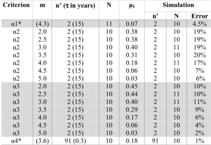
6.3 3-D von Neumann’s neighbourhood, r=1
As an example of interaction in three dimensions, the von Neumann’s neighbourhood of radius 1 is studied (Fig. 2g). The catalogue, is this case, is divided not only for the latitude and longitude, but for the depth too. Firstly, according to the α1 criterion (Table 3), if a cell is inactive, it will go on being inactive with a 85–99% probability; an active one has more than 50% probability of activation in the future if it has three or more neighbouring active cells. Otherwise, it will remain inactive at a next interval of time. The characteristic magnitude is m=4.3.
For the α2 criterion, and for any magnitude, a cell remains inactive with about a probability of 98% if no other cell in its neighbourhood is previously active. The probability of activation increases with the number of neighbouring active cells; if it has three or four, there is a 50% probability for activation, and 90% if there are six. This occurs until m=4.0, where an inactive cell is more likely to remain inactive, inde-pendently on the number of neighbouring active cells. This can be interpreted as that the higher energy releases occur al-ways at the same sites. However, if a cell is active, the next interval of time will be more likely to be inactive if there are less than two neighbouring active cells; with two active cells, the estimated probability of activation is 70%, and increases until 100% where there are six.
Table 3. Von Neumann’s neighbourhood (r=1, 3-D): activation cri-terion, threshold energy-magnitude (m), number of time intervals (n0), with the corresponding time length τ , and number of bins (N ) for the maximum of the mutual information (µI)in bits; n0and N used for the simulation, and its error. (*) With the abridged cata-logue. Simulation Criterion m n’ (ττττ in years) N µI n' N Error α1* (4.3) 2 (15) 11 0.07 2 10 4.5% α2 2.0 2 (15) 10 0.38 2 10 19% α2 2.5 2 (15) 10 0.38 2 10 19% α2 3.0 2 (15) 10 0.40 2 11 19% α2 3.5 2 (15) 10 0.31 2 10 20% α2 4.0 2 (15) 10 0.18 2 11 17% α2 4.5 2 (15) 10 0.06 2 10 7% α2 5.0 2 (15) 10 0.03 2 10 6% α3 2.0 2 (15) 10 0.45 2 10 10% α3 2.5 2 (15) 10 0.44 2 11 10% α3 3.0 2 (15) 10 0.40 2 11 11% α3 3.5 2 (15) 10 0.29 2 10 9% α3 4.0 2 (15) 10 0.17 2 10 6% α3 4.5 2 (15) 10 0.06 2 10 4% α3 5.0 2 (15) 10 0.03 2 10 2% α4* (3.6) 91 (0.3) 10 0.18 91 10 1%
With the α3 criterion the results are: if a cell is initially in-active, has a 98% probability of remaining inactive if there is no neighbouring active cell. This percentage diminishes and, when there are three or more surrounding active cells, the probability of activation is of 60%, increasing with the in-crease of the surrounding activity. Otherwise, if a cell is pre-viously active, has 80% probability of desactivation if there are less than two neighbouring active cells; if there are two or more, the probability of remaining active increases with the number of neighbouring active cells (from 70% to 100%). This behaviour is carried out until m=3.0; for higher mag-nitudes, when a cell is initially inactive, it is more likely to continue inactive. Also, the probability of activation for the active cell decreases with an increasing magnitude.
Finally, according to the α4 criterion, the mean energy to be surpassed is calculated to be the one corresponding to a magnitude of 3.6, and the seismicity is clearly clustered. The most probable is that an inactive cell remains inactive, and an active one continues being active, with a probability around 95% in both cases.
6.4 2-D von Neumann’s neighbourhood, r=2
So far, the analysis (in 2-D or 3-D) of interaction has cor-responded to the so-called “nearest neighbouring neighbour-hoods”. Here we study other neighbourhood where there is an interaction of longer range. It is composed by two parts: the nearest one, similar to the Moore’s neighbourhood of radius 1, and other, the far-out one, with four cells cross-disposed (Fig. 2b). The expression for the mutual informa-tion in this case is:
µI = 1 X i=0 1 X j =0 8 X k=0 4 X l=0
p(i; j, k, l)log2 p(i; j, k, l)
Table 4. Von Neumann’s neighbourhood (r=2, 2-D): activation cri-terion, threshold energy-magnitude (m), number of time intervals (n0), with the corresponding time length τ , and number of bins (N ) for the maximum of the mutual information (µI)in bits; n0and N used for the simulation, and its error. (*) With the abridged cata-logue. Simulation Criterion m n’ (ττττ in years) N µI n' N Error α1* (4.6) 3 (10) 10 0.26 3 10 8% α2 2.0 18 (1.7) 10 0.59 18 10 19% α2 2.5 18 (1.7) 10 0.59 18 10 19% α2 3.0 6 (5) 10 0.58 9 11 21% α2 3.5 2 (15) 12 0.60 6 11 20% α2 4.0 2 (15) 10 0.65 7 10 20% α2 4.5 2 (15) 10 0.47 6 10 15% α2 5.0 2 (15) 10 0.19 5 10 9% α3 2.0 18 (1.7) 10 0.59 18 10 19% α3 2.5 18 (1.7) 10 0.59 18 10 20% α3 3.0 6 (5) 10 0.58 6 11 18% α3 3.5 2 (15) 10 0.60 8 11 24% α3 4.0 2 (15) 10 0.64 7 10 20% α3 4.5 2 (15) 12 0.42 6 10 17% α3 5.0 2 (15) 10 0.19 5 10 9% α4* (4.1) 48 (0.6) 10 0.48 48 10 1%
with p(i; j, k, l) being the joint probability of past and future states, and p(i)p(j, k, l) a distribution of independent states;
irepresents the state of the central cell in the future and j its past state, with k nearest and l far-out neighbouring active cells, in the past.
With the α1 criterion, it can be observed that the cells are clustered, and there is not much interaction with the four cross-disposed cells. This can be due to the low number of cells involved, but the models with more cells behave the same. So the model for N =10 is chosen (Table 4). If a cell is inactive, it will continue inactive with an averaged probabil-ity of 90%; an active cell with a nearest active and one or two far-out active cells has 100% probability of continuing active (if there is no far-out active cell, it will be inactive); if there are two active cells it is more likely that it remains inactive, and, if it has three or four, with complete probability it will continue to be active. The characteristic magnitude is m=4.6, approximately. It has to be noted that the best model is equal to the one obtained with the Moore’s neighbourhood.
For the α2 criterion, and m=2.0–2.5, if a cell is inactive, and it has less than five nearest neighbouring active cells, it will continue inactive in most of the cases (80%); when there are active five nearest cells and also three or more external ones, it will activate in the future with 60–80% probability; starting from six nearest neighbouring active cells, in most of the cases the configurations have more probability of ac-tivation in the future. If a cell is active, it will be inactive if it has less than one nearest and two external active cells (70% probability of desactivation); otherwise, in general, the cell will go on being active, with high probability (∼70– 90%). For m=3.0, an inactive cell, with less than four nearest and three external active cells will remain inactive (60–90% probability, diminishing with the increasing of active cells); for most of the other configurations, the activation or
desac-tivation oscillates around the 50% probability. If the central cell is active, it needs, at least, other nearest and two exter-nal neighbouring active cells to continue being active. As the number of neighbouring active cells increases, the probabil-ity rises too, until 100%, when all the cells are active. For
m=3.5, one inactive cell will go on being inactive with high probability (70%), unless there were four nearest and three external active cells (70% probability of activation). When the central cell is active it does not go on being active until it has two nearest and two external active cells. With m=4.0– 5.0, an inactive cell will remain inactive, independently on the surrounding activity (80% probability in average); if the cell is active it is more likely to become inactive (60%), if it has less than two nearest and one external active cells. With these magnitudes there is difficulty in choosing an adequate model, because these energy levels are reached in set places, and the configurations with high number of active cells are not present. In general, inactive cells remain inactive (90% probability), and the activation is produced when the central cell is active, and there is a total of four neighbouring active cells.
And for the α3 criterion we have: with m=2.0–2.5, the simulation for the global maximum predicts that if a cell is initially active, it will continue active with high probability (80–90%) in most of the cases. However, when the central cell has five or more nearest and three or more external active cells, the probability of activation in the next time interval is 70%. With regard to the initially active cells, they do not set-tle on activity until they have more than three nearest active cells. Thus, the activation probability increases with the total number of active cells (60–95%). With m=3.0, if a cell is active, it is more likely (∼80%) that it changes to inactive. If the central cell has seven or eight nearest and more than two external active cells, the probability of activation is 80% in average. However, if a cell is previously active, it will not be active in the future if it has less than two nearest and two ex-ternal active cells. The probability of activation is, then, 90% in average. For m=3.5, in most of the cases, when the central cell is inactive, it goes on being inactive (70–100%). This does not occur with: four nearest and three external active cells (60% probability of activation), five nearest and three external ones (100% to be active), six nearest and one ex-ternal active cells (70% for the activation), six nearest and three external ones (100%), and with seven nearest and two or four external active cells (70% and 100% probability of activation, respectively). It should be noted that the number of involved cells is high (seven or more). Likewise, an active cell will remain active (more than 80% probability) if there are five or more neighbouring active cells, either nearest or external ones. If this does not occur, it is most likely the in-activity, mainly with the low number of neighbouring active cells (two or less). When m=4.0, an inactive cell will remain inactive, independent of the surrounding activity, with a high probability (∼80%); if it is active, it will be inactive for less than three neighbouring active cells. It is necessary at a min-imum that an external active cell to be active in the future. In general, this occurs when the total number of active cells is
A. Jim´enez et al.: A probabilistic seismic hazard model based on cellular automata and information theory 11 six or more. For m=4.5, an inactive cell will go on being
in-active with 80–100% probability; an in-active one will continue active if it has two nearest and one or two external active cells (100%). Otherwise, it is more likely to be inactive in the fu-ture. It has to be noted that the configurations with five or more active cells has not been presented, because of the high magnitudes involved. Finally, with m=5.0, if a cell is inac-tive, it remains inactive (90% probability), and if it is acinac-tive, it will continue active with three nearest neighbouring active cells, or with only one external neighbouring active cell. For the other cases, it is more likely that the cell will be inactive (80% in average). Neither this magnitude presents situations with too many cells active (always three or less).
With the α4 criterion, a cell will go on being active or inactive (95% probability) independently of the other cells. Configurations with more than five active cells have not been presented. The characteristic energy corresponds to a mag-nitude of 4.1.
7 Discussion and conclusions
It can be seen that the best configurations (n0and N ) for all the neighbourhoods studied have the lowest resolution tried:
Nis regularly 10 or 11 (only a few are 12 or more). With re-gard to the number of interaction times, n0, they are quite similar for both von Neumann’s and Moore’s neighbour-hoods of radius 1. The time interval τ increases, within each criterion, with the threshold energy-magnitude. The mutual information rises with the number of cells in the neighbour-hood (in order: von Neumann’s radius 1, Moore’s radius 1, and von Neumann’s radius 2, in 2-D), but the errors are sim-ilar.
With the von Neumann’s radius 2, the configurations and maps are very similar to those of Moore’s radius 1 (Fig. 6); and that tell us that the nearest activity to the cell is the most important for the future of the state of the cell. Since the simulation errors are similar, as well as the results, we can say that it is better to use Moore’s, because, on the one hand, the computation time is smaller and, on the other hand, it is simpler than the von Neumann’s, and so the interpretation is easier. Also, bearing this in mind, a study with another template with a higher number of cells, as the Moore’s radius 2, would not contribute to obtaining better results.
However, it is very difficult to decide between the Moore’s and the von Neumann’s of radius 1. First, the errors are sim-ilar, and also the values for n0and N , so that the best neigh-bourhood would be the simpler one (von Neumann’s); but the mutual information is always higher in the Moore’s; for ex-ample, with the α1 criterion (using the abridge catalogue) the maximum µI is 0.13 bits for the von Neumann’s, and 0.22 bits for the Moore’s. This behaviour is the same in general for all the criteria, the reason being that the Moore’s neigh-bourhood is larger. Because of the addition of the energy from all the cells involved, if the von Neumann’s were cho-sen, the preferred directions would be N-S and E-W, and that could not be realistic. Therefore, because of the isotropy and
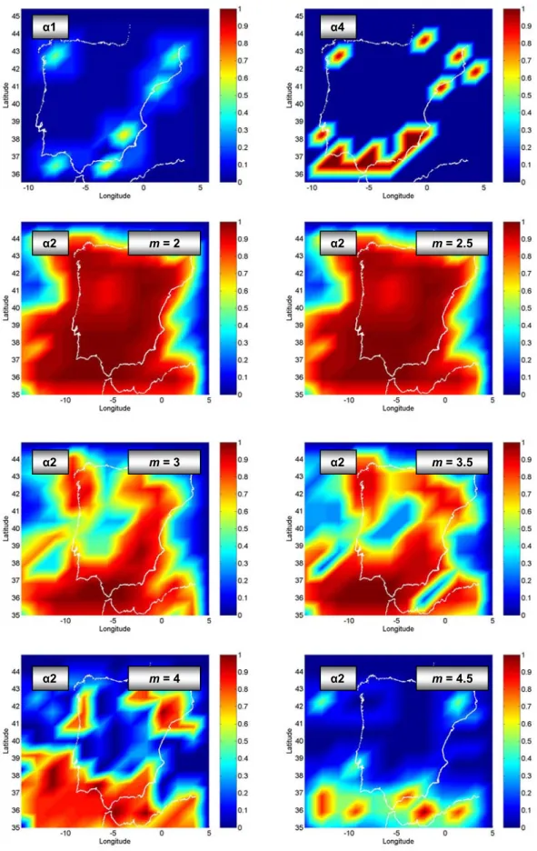
the higher amount of information, the Moore’s is considered to be the best neighbourhood for the 2-D models, and the Probabilistic Seismic Hazard Maps for the Iberian Peninsula (Fig. 6) correspond to those obtained with this neighbour-hood.
With regard to the 3-D neighbourhood, the resolution found is poor (N =10), and the interaction time τ is around 15 years. The advantage of this template is that it provides a finer localization of the seismicity (the depth). However, the simulations are worse than those of the 2-D neighbourhoods. In general, the Probabilistic Seismic Hazard Maps ob-tained by taking into account the complete catalogue indi-cate that the main activity (with energy releases higher than the average) is predicted in northern Algeria, northern Mo-rocco and the Atlantic Ocean near Lisbon. If these zones are excluded (abridged catalogue), the maximum activity is lo-cated in the south of Iberia (mainly, the gulf of C´adiz, the coasts of M´alaga and Almer´ıa, and Murcia), Galicia, and the coastal Catalonian range, over the next 7–10 years, accord-ing to the α1 criterion. Takaccord-ing into account the α4 criterion, the western Pyrenees is also a zone of high activity. These zones are, effectively, the main seismogenetic regions in the Iberian Peninsula.
With the three-dimensional template evaluated, from the
α1 and α4 criteria (with the abridged catalogue) it can be de-duced that the main activity will occur at the same sites as in the two-dimensional cases. The important difference be-ing that this analysis shows that this activity is concentrated in the first 15 km of the crust, and that the deepest activity is found at Tarifa. From α2 and α3, it is seen that the ac-tivity is mainly shallow; starting from m=4.0, the maximum probability of seismic events deeper than 30 km is found in the southern Iberian Peninsula. In the Pyrenees and Galicia the probability is that only shallow earthquakes occur up to a depth of 30 km and with a magnitude up to m=4.0. This is in agreement with the observed seismicity (NEIC; Henares et al., 2003). For a magnitude threshold of 5.0, the region of highest seismic hazard is the northern Algeria and the Mo-roccan coast, with a maximum depth of 15 km. Two impor-tant earthquakes have occurred in these places, with a magni-tude higher than 6.0: the Algerian, in May 2003, with a depth less than 20 km, and the one of Alhoceima, in February 2004, with a depth less than 5 km.
The maps obtained from the α1 and α4 criteria with the abridged catalogue (whose characteristic magnitude was 4.0, approximately) are similar to those calculated from the α2 and α3 criteria for a magnitude threshold of 4.0; the maps are also similar using the complete catalogue (but with a magni-tude threshold of 5.0 for the α2 and α3 criteria, because the characteristic magnitude for the α1 and α4 criteria was 5.0 using the complete catalogue). So both kind of criteria are consistent.
An interesting result for all the templates is that the high-est transmission of information is found at the lowhigh-est reso-lutions. This is the consequence of modelling a large and complex area with regions of different tectonic behaviour. The models have to fit the whole area, so the most reliable
α4 α1 α2 m = 2 α2 m = 2.5 α2 m = 3 α2 m = 3.5 α2 m = 4 m = 4.5 α2
A. Jim´enez et al.: A probabilistic seismic hazard model based on cellular automata and information theory
Moore’s neighbourhood, r = 1.
13 α3 α3 m = 4.5 m = 5 m = 4 m = 3.5 α3 α3 m = 2 m = 5 α3 α2 m = 3 m = 2.5 α3 α340
Fig. 6. Continued.information is present when the cells represent zones of ho-mogeneous seismicity and the local effects are removed by making an average. A similar result was obtained by Lom-nitz (1994), who showed that the Hurst’s analysis should not be applied to large complex regions, because the localized effects superimpose each other in such a way that statistics is destroyed. To avoid this, smaller areas should be studied be-cause, as it has been shown, more complex neighbourhoods do not improve the results. This could be the reason for the different time interaction between the 2-D and 3-D models. In 3-D, when considering the depth, the statistics of the cells is shown to have more differences. The seismicity is mostly shallow, contributing more to the energetic weight; the deep-est earthquakes happen to have higher characteristic time but there are few so that, for 2-D models, these events have no influence on the statistics.
The time intervals increase τ when higher energies are considered, as could be expected. The models obtained tend to continue the activity, in agreement with the observed clus-tering of the seismicity (Aki, 1956; Pe˜na et al., 1993). The Hurst’s analysis, by using the accumulated energy, shows an inherent unpredictability in the future states. The Hurst’s ex-ponent found is of 0.48±0.02, in agreement with the one ob-tained by Ogata and Abe (1991). This means that the best prediction is to repeat the last state, and it is related to the inability of the CA calculated for predicting sudden changes in the patterns.
From the calculated b and a/b values from the Gutenberg-Richter’s law, it can be deduced that the region under study is highly active, and that the events with a lower magnitude are more likely to occur. This is due to the high hetero-geneity of the crust and is in agreement with the previous results, which show that most of the earthquakes are bellow magnitude m=5.0, and with other studies made in the zone (Bezzeghoud and Buforn, 1999).
It has to be noted that our proposed method includes the possibility of quantifying the errors (other probabilistic methods used for seismic hazard studies do not provide these error estimations), because of the discretization of the prob-lem and the use of the Hamming distance. Although the cor-relation functions from real and simulated patterns are a good way to establish differences between them, they are more qualitative than the Hamming distance, which has resulted in a powerful tool, mainly because the former functions have been found to be very close to each other in most of the cases. The errors of the presented models (neighbourhood and con-figurations) are different for each activation criterion. For the
α1 one, it oscillates between 5% and 10%; 10–20% for the
α2 and α3 criteria and 1 or 2% for the α4 one. This is due to the fact that the seismicity events are located almost al-ways at the same sites, and the α1 and α4 criteria signal the main seismogentetic zones, as explained before. Besides, the
α4 criterion is built from the whole catalogue (complete or abridge) until the time considered (as macroseismic studies do), and, if an important seismic event occurs in a region, that region will from then on be considered as seismically active (note that the energy release has to be above the
aver-age in the whole area). On the other hand, the α1 criterion only takes into account the amount of energy in a time in-terval, so that the patterns are more dynamic, and not all the zones interact synchronically (and because of that the mu-tual information has to be used); therefore, the errors have to be higher. The other criteria (α2 and α3) try to predict the energy release in an absolute way, so that the errors are the highest. It is well-known that the prediction of events of a certain magnitude is, for the present, unreliable in most of the cases, although some successful predictions have been made (Sykes and Nishenko, 1984; Scholz, 1985; Nishenko, 1989; Nishenko et al., 1996; Wyss and Burford, 1985; Pur-caru, 1996; Kossobokov et al., 1997; Tiampo et al., 2002; Keilis-Borok, 2000).
In spite of the errors, the recorded seismicity after the data used coincides to a large extent with the seismic hazard maps proposed in this paper. Comparing them with the ESC-SESAME Unified Seismic Hazard Model for the European-Mediterranean Region (Jim´enez et al., 2001), it can be seen that they indicate the same sites where the highest magnitude events are more likely to occur, and that these are of a mod-erate magnitude. The α4 criterion is the closest one to other macroseismic studies found in literature. With regard to the other criteria, they provide a more dynamic seismic hazard assessment.
So we can conclude that a simple model based on stochas-tic Cellular Automata for estimating the seismic hazard in a probabilistic way is developed. The activity of a zone is calculated from its previous activity and from the surround-ing one. The released energy has been processed as a dis-crete variable, both spatially and temporally, to predict, from a probabilistic point of view, the energy to be released in the future at that zone. From a theoretical point of view, the maximization of the mutual information between previous and future states at a site is an adequate and consistent way in choosing the highest dependence between them.
The method has been applied to the seismic catalogue of the Iberian Peninsula (from 1970 to 2001). Different acti-vation criteria have been evaluated. The α1 and α4 provide a rough prediction of sites where the main seismic activity will be presented. The α2 and α3 criteria delineate the areas where a certain energy will be surpassed. In all cases, the inclusion of the energy of the events is crucial for the regions where there are few earthquakes, but with a high magnitude; for these regions, 2-D and 3-D neighbourhoods have been tested. For 2-D, the Moore’s of radius 1 has been chosen, because of the higher amount of information and isotropy; with the 3-D (von Neumann’s of radius 1) the Probabilistic Seismic Hazard Maps can be calculated taking into account also the depth of the events. Therefore, our method is truly adequate for the study of the seismic hazard in a probabilis-tic way; it is solid and logical in characterizing the spatio-temporal evolution of seismic activity.
Acknowledgements. The authors thank B. Barry, whose comments
and English revision led to an improvement of this study. This work was partially supported by the MCYT project