Open Access Full Text Article
Research Article
1
Training Center of Electrical Engineering, School of Electrical Engineering, Hanoi University of Science and Technology
2
Electrical Engineering and Computer Science Department of the University of Liège, Belgium
Correspondence
Vuong Dang Quoc, Training Center of Electrical Engineering, School of Electrical Engineering, Hanoi University of Science and Technology
Email: [email protected]
Using edge elements for modeling of 3-D magnetodynamic
problem via a subproblem method
Vuong Dang Quoc
1,*, Christophe Geuzaine
2Use your smartphone to scan this QR code and download this article
ABSTRACT
Introduction: The mathematical modeling of electromagnetic problems in electrical devices are
often presented by Maxwell's equations and constitutive material laws. These equations are par-tial differenpar-tial equations linked to fields and their sources. In order to solve these equations and simulate the distribution of magnetic fields and eddy current losses of electromagnetic problems, a subproblem method for modeling a 3-D magnetodymic problem with the b-conformal formula-tion is proposed. Methods: In this paper, the subproblem method with using edge finite elements is proposed for coupling subproblems via several steps to treat and deal with some troubles regard-ing to electromagnetic problems that gets quite difficulties when directly applyregard-ing a finite element method. In the strategy subproblem method, it allows a complete problem to define into sev-eral subproblems with adapted dimensions. Each subproblem can be solved on its independent domain and mesh without performing in whole domain or mesh. This easily supports meshing and decreases computing time. Results: The obtained results, the subproblem method with edge elements indicates magnetic flux densities and the eddy current losses in the conducting region. The computed results is also compared with the measured results done by other authors. This can be shown that there is a very good agreement. Conclusion: The validated method has been successfully applied to a practical test problem (TEAM Problem 7).
Key words: Eddy current, Magnetic field, TEAM problem 7, b-conformal formulation, finite
ele-ment method, subproblem method
INTRODUCTION
As we have known, the mathematical modeling of electromagnetic problems in electrical devices are often presented by Maxwell’s equations and constitutive material laws. These equations are partial differential equations (PDEs)1,2linked to fields and their sources (such as: magnetic and electric fields, eddy current losses).
In order to solve these equations and simulate the distribution of magnetic fields and eddy current losses, many authors have been recently used a finite element method (FEM) for magnetodynamic problems. But, the directly application of the FEM to an actual problem is still quite difficult3,4when the dimension of the computed conducting domains is very small in comparison with the whole problem.
In order to overcome this drawback, many authors have been recently proposed a subproblem method (SPM) to divide a complete problem into subproblems (SPs) in one way coupling5–7. However, this proposal was done for thin shell models, where appearing errors near edge and corner effects5–7.
In this study, the SPM is expanded for coupling SPs via two steps with using edge finite elements (FEs). The scenario of this method is also based on a SPM5, instead of solving a complete model (e.g, stranded inductors and conducting regions) in a single mesh, it will be split into several problems with a series of changes. This means that the problem with a stranded inductor (coil) alone is first solved, and then the second problem with conducting regions is added. Thus, the complete solution is finally defined as a superposition of the SP solutions. From this SP to another is constrained by interface conditions (ICs) with surface sources (SSs) or volume sources (VSs), that express changes of permeability and conductivity material in conducting regions.The developed method is performed for the magnetic flux density formulation and is illustrated on a practical test problem (TEAM problem 7)3.
Cite this article : Dang Quoc V, Geuzaine C. Using edge elements for modeling of 3-D magnetody-namic problem via a subproblem method. Sci. Tech. Dev. J.; 23(1):439-445.
History •Received: 2019-10-16 •Accepted: 2019-12-10 •Published: 2020-02-20 DOI : 10.32508/stdj.v23i1.1718 Copyright
© VNU-HCM Press. This is an open-access article distributed under the terms of the Creative Commons Attribution 4.0 International license.
SPM IN A MAGNETO DYNAMIC PROBLEM
A magnetodynamic problem is defined in a studied domainΩi, with boundary∂Ωi=Γ = Γh∪ Γb.
The conducting region ofΩ is denoted Ωc
and the non-conducting oneΩc c,i,
withΩC= Ωc,i ∪ ΩCc,i.
The eddy current belongs toΩC, whereas stranded inductors is defined inΩCc. The Maxwell’s equations
together with the following constitutive relations are7–10
curl hi= ji,divbi= 0, curlei=−∂tbi (1a-b-c) hi=µi−1bi+ hs,i, ji=σiei+ js,i (2a-b) n× hi|Γh = jf ,i, n× bi|Γb = kf ,i, (3a-b) where hiis the magnetic field, biis the magnetic flux density,
eiis the electric field, jiis the electric current density,µiis the magnetic permeability,σiis the electric
conductivity and n is the unit normal exterior toΩi.
The fields jf ,i and ff ,iin (3a) and (3b) are SSs and consider as a zero for classical homogeneous boundary
conditions. From the equation (1b), the field bican be obtained from a magnetic vector potentialαivia a
bi = curl ai. (4)
Taking (4) into (1c), it gets curl (ei +∂tai) = 0, that leads to the presentation of an electric scalar potentialν
through
ei = −∂tai− gradνi. (5)
The sources hs,iin (2a) and js,iin (2b) are VSs that can be expressed as changes of a material property in5–7.
For example, the changes of materials from SP q (i = q) to SP p (i = p) can be defined via VSs bs,p
and js,p, i.e.
hs,p = (µ−1p µq−1) bu, js,p = (σp− σq) eq, (6a-b)
for the updated relations, i.e.
hu+ hp= (µ−1p (bu+ bp) and jq+ jp=σpeu+ ep).
FINITE ELEMENT WEAK FORMULATION
Magnetic flux density formulationBy starting from the Ampere’s law (1a), the weak form of bi-formulation of SP i(i≡ q, p) is written as 4 − 7
(µi−1bi, curl a′i)Ω− (σiei, a′i)Ωc +⟨n × hi, a′i⟩ = ( js,i,a′i)Ωs,∀ a′i∈Fe0 (curl,Ω). (8) Combining the magnetic vector potential aiand the electrical field eidefined already by (4) and (5), one has
(µi(−1)curl ai, curl ai′)Ωi+ (σ∂tai, ai′)Ωc,i+ (hs,i, curl a′i)Ωi + ( js,i, a′i)Ωi+ (σigradν,a′i)Ωi+⟨n × hi, a′i⟩Γh = ( js, a′i)Ωs,i),∀a′i ∈ Feo(curl,Ωi),
(9) where F0
e(curl,Ωi)is a function space defined onΩicontaining the basis functions for aias well as for the
test function a′i(at the discrete level, this space is defined by edge FEs; notations (·, ·) and < ·, · > are respectively a volume integral in and a surface integral of the product of their vector field arguments. The surface integral term onΓh(
⟨
bxhi, a
′ Γh
⟩
in (9) is defined a homogenous Neumann BC, e.g. imposing a symmetry condition of ”zero crossing current”, i.e.
n x hlΓh = 0 ⇒ n · hilΓh= 0 ⇔ n · jilΓh = 0. (10) The obtained solutions by solving equation (9) with a stranded inductor alone is then considered as VSs for solving the second problem (with an added conducting region) via the volume integrals
(hs,i,curl a
′
i)Ωiand ( js,i,a ′
Discretization of Edge FEs As presented in1,7, each edge e
i j={i, j} linked to the vector field is defined as Sei, j= pjgrad (∑ r∈NF, j, − ipr )− pigrad (∑r∈N F,i, − j pr), (11) where N
F,m,−nis the set of nodes in the facet containing evaluation point x. This means that it contains node m
without node n, and each facet is uniquely determined for three-edge-per-node elements (Figure1), where either a triangular or a quadrangular facet is involved. The set N
F,m,−ndepends on point x, which can be either {{m},{o},{p}} or {{m},{o},{p},{q}}, respectively. It should be noted that vector field Sei jis defined as a zero in all the elements without linking to edge ei j. The vector field space created by sei j,∀ e ∈ E, is denoted by S1.
Figure 1: Definition of the facet associated with notationNF, j,i−.
Basis function of Edge FEs
According to definition of basis functions, the value of Sei jis defined as 1 along the edge ei j, and equal to 0 along other edges i.e.
Hi
jsi· dl =δi, j,∀ i, j ∈ E, (12)
whereδi, j= 1 i f i = j andδi, j= 0 i f i̸= j.
This property shows up variations of functionals and included that functions Sei jfrom base for the space it generates. This is then called an edge base function. The associated FEs and celled edge FEs. The edge function is helpful to check some of its characteristic. The vector field
grad P
F,m,−n= grad(∑r∈N
F,m,−n
pr), (13)
involved in the expression (11), need to be analyzed at first. The characteristic of continuous scalar field,
P
F,m,−n=∑r∈N
F,m,−n
pr, (14)
is equal to 1 at very point in the facet linked to the N
F.m.−n, which is a property of the nodal functions. The
vector field of the product of pmand (13),
pmgrad (∑r∈N
F,m,−n
pr) (15)
is developed now. This field is united with the edge{m,n}. As soon as the function pmis considered, it is
defined as a zero on all the edges containing point x, without being incident to node{m}. Thus, the value of (15) is defined as a zero along the all the edges without emn. The vector fields defined in (15) is equal to zero
on them as shown in Figure 3. The association of the fields in (15) combined with edges{ j,i} and {i, j}, as in (11), gives a vector field which has the announced properties Sei jas in (15) (Figure2). This also means that circulation along edge ei jis equal to 1 with this edge and is equal to zero with others.
Figure 2: Geometric interpretation of the edge function Se.
APPLICATION TEST
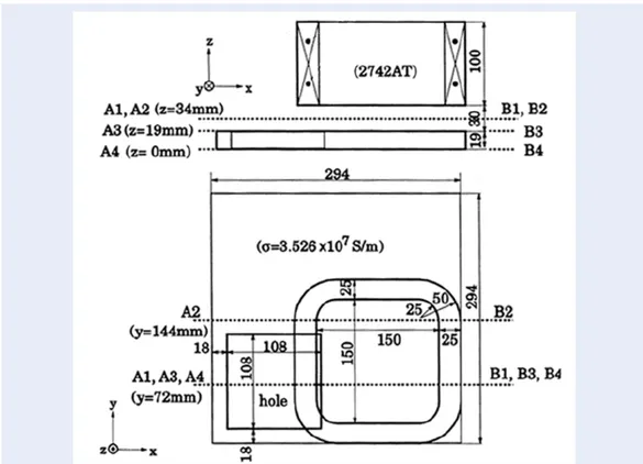
The practical test problem is a 3-D model based on the benchmark problem 7 of the TEAM workshop including a stranded inductor (coil) and an aluminum plate3(Figure3).
The coil is excited by a sinusoidal current which generates the distribution of time varying magnetic fields around the coil. The relative permeability and electric conductivity of the plate are
µr,plate= 1,σr,plate= 35.26 MS/m, respectively.The source of the magnetic field is a sinusoidal current
with the maximum ampere turn being 2742AT. The problem is tested with two cases of frequencies of the 50 Hz and 200 Hz.
Figure 3: Modeling of TEAM problem 7:coil and conducting plate3, withµ
r,plate= 1,σr,plate= 35.26MSm.
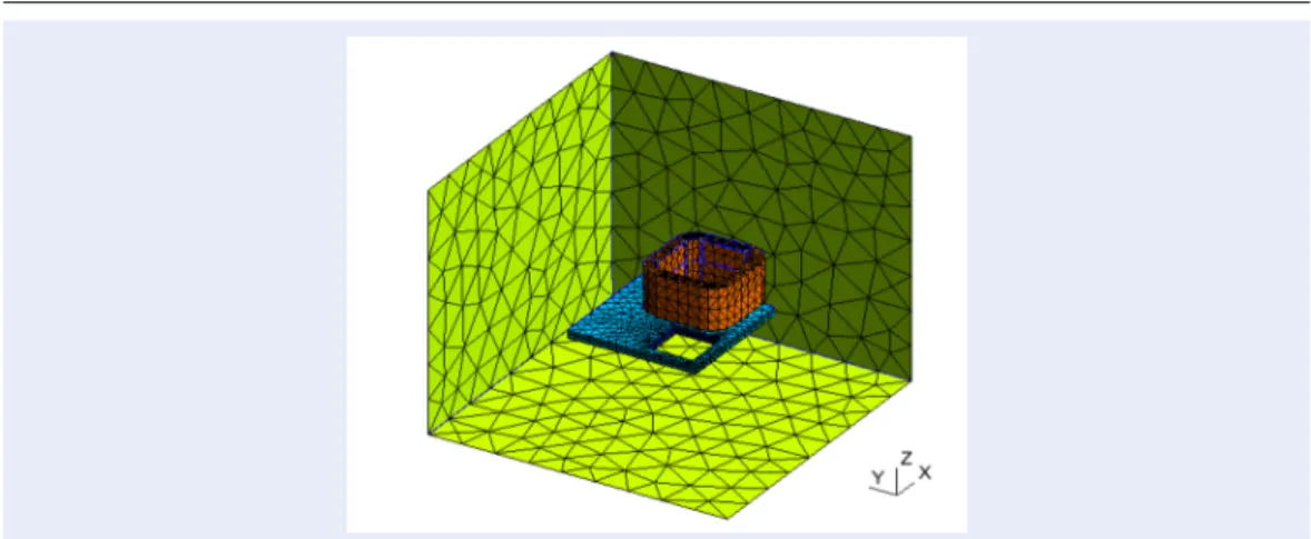
The 3-D dimensional mesh with edge elements is depicted in Figure4. The problem with the coil alone is first considered. The distribution of magnetic flux density generated by the excited electric current in the coil is pointed out in Figure 5. The computed results on the of the z-component of the magnetic flux density along
Figure 4: The 3-D mesh model with edge elements of the coil and conducting plate, and the limited
bound-ary.
Figure 5: Distribution of magnetic flux density generated by the excited sinusoidal current in the coil, with
µr,plate= 1,σr,plate= 35.26MSm and f = 50 Hz.
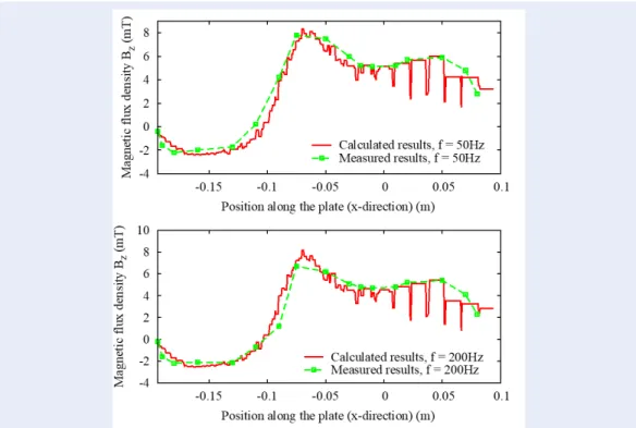
the lines A1-B1 and A2-B2 (Figure3) is checked to be close to the measured results for different frequencies of exciting currents (already proposed by authors in [3]) are shown in Figure6. The mean errors between calculated and measured methods7on the magnetic flux density are lower than 10%. This can be demonstrated that the results obtained from the SPM is completely suitable and accepted.
The y component of the varying of the eddy current losses with different frequencies (50 Hz and 200 Hz) along the lines A3-B3 and A4-B4 (Figure3) is shown in Figure7. The computed results are also compared with the measured results as well3. The obtained results from the theory modeling are quite similar as what measured from the measurements. The maximum error near the end of the conductor plate on the eddy currents between two methods are below 20% for both cases (50 Hz and 200 Hz). This is also proved that there is a very good validation between the SPM and experiment methods3.
CONCLUSION
The extended method has been successfully computed the distribution of magnetic flux density due to the electric current following in the coil, and the eddy current losses in the conductor plate. This aim has been achieved by a detailed study of the magnetic flux density formulation and finite element edges via SPM. With the obtained results, the method with edge element also indicates that where the hotpot occurs in the conducting regions developed in another topic. The method has been also successfully validated to the actual problem (TEAM problem 7).
Figure 6: The comparison of the calculated results with the measured results at y =72mm, withµr,plate=
1,σr,plate= 35.26MSm and di f f erent f requencies.
Figure 7: The comparison of the calculated results with the measured results at z = 19mm, withµr,plate=
COMPETING INTERESTS
The authors declare that there is no conflict of interest regarding the publication of this article.
AUTHORS’ CONTRIBUTIONS
All the main contents and the obtained results of the paper have developed by the author and co-author (Prof. Christophe Geuzaine as mentioned in the paper).
REFERENCES
1. Geuzaine C, Dular P, Legros W. Dual formulations for the modeling of thin electromagnetic shells using edge elements. IEEE Trans Magn. 2000;36(4):799–802. Available from:https://doi.org/10.1109/20.877566.
2. P D, Q V, Dang RV, Sabariego L, Krähenbühl, Geuzaine C. Correction of thin shell finite element magnetic models via a subproblem method. IEEE Trans Magn. 2011;47(5):158–1161. Available from:https://doi.org/10.1109/TMAG.2010.2076794.
3. Gergely KOVACS and Miklos KUCZMANN, Solution of the TEAM workshop problem No.7 by the finite Element Method. Approved by the International Compumag Society Board at Compumag-2011.
4. S K, P S, V SR, D VQ, Wulf MD. Influence of contact resistance on shielding efficiency of shielding gutters for high-voltage cables. IET Electr Power Appl. 2011;5(9):715–720. Available from:https://doi.org/10.1049/iet-epa.2011.0081.
5. D VQ, Dular P, Sabariego RV, Krähenbühl L, Geuzaine C. Subproblem approach for Thin Shell Dual Finite Element Formulations. IEEE Trans Magn. 2012;48(2):407–410. Available from:https://doi.org/10.1109/TMAG.2011.2176925.
6. D VQ, Sabariego RV, Krähenbühl L, Geuzaine C. Subproblem Approach for Modelding Multiply Connected Thin Regions with an h-Conformal Magnetodynamic Finite Element Formulation. EPJ A. 2013;63(1):xxx–xxx.
7. Dang Quoc Vuong. Modeling of Electromagnetic systems by coupling of Subproblems-Application to Thin Shell finite element magnetic models, Ph.D. Thesis, University of Liege, Belgium.
8. D VQ. Modeling of Magnetic Fields and Eddy Current Losses in Electromagnetic Screens by A Subproblem Method. TNU Journal of Science and Technology,. 2018;194(1):7–12.
9. Q VD. From 1D to 3D for Modeling of Magnetic Fields via a Subproblem Method. TNU Journal of Science and Technology. 2019;200(7):63–68.
10. V DQ, Q ND. Coupling of Local and Global Quantities by A Subproblem Finite Element Method – Application to Thin Region Models. Advances in Science, Technology and Engineering Systems Journal (ASTESJ). 2019;4(2):40–44.

![[PDF] Tutoriel Arduino Simulink Matlab | Cours PDF](data:image/gif;base64,R0lGODlhAQABAIAAAP///wAAACH5BAEAAAAALAAAAAABAAEAAAICRAEAOw==)