Asyiiimetrv Risk,
$tate
Variables arid $touhastic Discount Factor
$pecificatioii
in
Asset Pricing iViodels
par
fousseni Chahi-Yo
Départerneiit de sciences économiques Faculté des arts et des scieHces
Thèse présentée à la Fàculté des études supérieures en vue de l’obtention du grade de
Fhilosophiae Doctor (Ph.D.) en sciences économiques
Octobre 2001
Q
C7<’- —de Montréal
Direction des bibliothèques
AVIS
L’auteur a autorisé [Université de Montréal à reproduite et diffuser, en totalité ou en
partie,
par quelque moyen que ce soit et sur quelque support que ce soit, et exclusivement à des fins non lucratives d’enseignement et de recherche, des copies de ce mémoire ou de cette thèse.L’auteur et les coauteurs le cas échéant conservent la propriété du droit d’auteur et des droits moraux qui protègent ce document. Ni la thèse ou le mémoire, ni des extraits substantiels de ce document, ne doivent être imprimés ou autrement reproduits sans l’autorisation de l’auteur.
Afin de se conformer à la Loi canadienne sur la protection des renseignements personnels, quelques formulaires secondaires, coordonnées ou signatures intégrées au texte ont pu être enlevés de ce document. Bien que cela ait pu affecter la pagination, il n’y a aucun contenu manquant. NOTICE
The author 0f this thesis or dissertation has granted a nonexciusive license allowing Université de Montréal to reproduce and publish the document, in
part
or in whole, and in any format, solely for noncommercial educational and research purposes.The author and co-authors if applicable retain copyright ownership and moral rights in this document. Neither the whofe thesis or dissertation, nor substantial extracts from it, may be printed or otherwise reproduced without the author’s permission.
In compliance with the Canadian Privacy Act some supporting forms, contact information or signatures may have been removed from the document. While this may affect the document page count, it does flot represent any loss of content from the document
Cette thèse intitulée:
Asynmietry Risk, State Variables aiid $tochastic Discount Factor
Specification
in
Asset Priciiig Models
présentée par
Fousseni Chabi-Yo
a été évaluée par un jury composé des persormes suivantes: Silvia Goncalves président. -rapporteur fric Renault directeur de recherche René Garcia codirecteur de recherche Bryan Campbell
membre du jury (Concordia University) Angelo Melino
exami riateur externe (University of Toronto) Yoshua Bengio
représentant du doyen de la Ff5
Ma thèse est centrée sur lintroduction (le l’asymétrie dans les modèles d’évaluation d’aetifs financiers et dans le choix de portefeuille. Dans le premier chapitre. nons examinons comment l’éc1nihbre (l’un marché financier révèle, à la fois par les ciuantités détenues à l’équilibre et par les prix, les préférences (les investisseurs pour trois types de caractéristique (les rendenients : leur espérance. leur variance et leur asymétrie. Dans le de1Lxième chapitre, en prenant en compte I’ asymétrie, nous déterminons mie nouvelle borne sur la variance (le tout facteur d’actualisation stochastique (SDF) qui valorise correctement les rendements d’actifs financiers et les gains (le pro— duits dérivés qui sont (les fonctions quadratiques (les gains d’actifs risqués. Dans le troisième chapitre, nous construisons une économie où les préférences des investisseurs et 1cm’ consonunation dépendent d’une variable d’état qui suit un processus de type Markovien à deux états et montrons que ce modèle économique produit et explique les énigmes de l’aversion pour le risque et du SDP mises en évi(lence par Jackwerth (2000. RFS). Dans le quatrième chapitre. nous proposons une ap proche pour l’évaluation (le prodmts dérivés par les arbres lorsqu’une variable (l’état non observable affecte le processus de prix du sous-jacent.1
Dans le premier chapitre, nous examinons comment l’équilibre d’un marché financier révèle, à la fois par les quantités détenues à l’équilibre et par les prix, les préférences des investisseurs po-ir trois types de caractéristique des rendements leur espérance. leur variance et leur asymétrie. Deux types d’approche sont utilisés pour cela. D’abord, en considérant une situation au voisinage (le la non-incertitude (expansion en petit bruit), on calcule les demandes des agents pom’ différents types d’actifs risqués. L’idée est de considérer un actif en offre non nulle, représentatif du portefeuille de marché, et des actifs dérivés en offre nette nulle mais dont les gains sont des fonctions non linéaires (lu portefeuille (le marché. On s’aperçoit alors que la demande d’actifs dérivés est précisément justifiée par le goût des investisseurs pour l’asymétrie .Au niveau (les prix, la rémunération du risque (lépend non seulement du bêta de marché, connue (lans un contexte moyenne—variance classique. mais aussi (11m coefficient de coas métrie par rapport au marché. Les conclusions obtenues par te premier chapitre (le cette thèse a été écrit en collaboration avec Dietrnar Leisen et Eric Renault Le delLxiètrle, troisième et le quatrième chapitre ont été écrits en collaboration avec René Garda et Eric Renault.
l’expansion en petit bruit peuvent ensuite étre retrouvées clans des contextes plus généraux grace à la définition d’un facteur d’actualisation stochasticiue adapté. Cette double approche peut etre ensuite étendue à iiri marché à cieux périodes où d’autres phénomènes d’asymétrie doivent étre pris en compte dans la dépendance temporelle des rendements d’une période à l’autre.
L’objet du deuxième chapitre est l’extension de l’approche des bornes de variance proposée par Ilansen et Jagannathan (1991, JPE). Alors ciue llansen and Jagamiathan (1991, JPE) caractérisent la variance minimale que doit avoir un facteur d’actualisation stochastique (SDF) susceptible de valoriser correctementmi ensemble donné d’actifs primitifs, nous considérons l’effet sur cette borne de variance de l’ajout de contraintes imposées par l’évaluation correcte des fonctions quaciratiques des gains de ces actifs primitifs. Nous approchons ainsi le problème de l’évaluation d’actifs dérivés dont les gains sont par définition des fonctions non linéaires des gains des actifs sous-jacents. II est alors éclairant de décrire la nouvelle frontière de variance ainsi obtenue dans un espace à trois dimensions mettant en jeu non seulement les rendements espérés et leur variance mais aussi leur coefficient d’asymétrie. De mème ciue la frontière de variance de Ilansen anci Jagannathan (1991, JPE) présente une relation de dualité avec la frontière efficiente moyenne-variance du choix optimal de portefeuille au sens de Markowitz (1952, Jf), la frontière ciue nous proposons peut
étre interprétée en ternies de choix de portefeuille par minimisation du risque sous contrainte non seulement de cotit et de rendement espéré, mais aussi d’une contrainte qui dépend de l’asymétrie du portefeuille. Nous montrons que la solution du problème de minimisation du risclue sous contrainte de coùt, du rendement espéré et d’asymétrie du portefeuille proposée par de Athayde et flores (2004, JEDC) est un cas particulier de notre problème de choix de portefeuille. En ce sens, notre travail donne uni nouvel éclairage à la cluestion du choix de portefeuille en présence de rendements asymétriciues.
Dans le troisième chapitre, nous présentons un modèle économnique avec changements de régime qui produit et explique les énigmes de l’aversion pour le risque et du SDF mises en évidence clans Jackwerth (2000, RFS). Nous construisons un modèle où les préférences des investisseurs et leur consommation dépendent d’une variable cfétat cmi suit un processus de type Markovien à cieux états et sinriulonis les prix d’options d’achat européennes. En utilisant la méthodologie proposée par
Jackwerth (2000, RFS), nous déduisons la fonction d’aversion absolue pour le risque et dii SDF pour chaque valeur de la richesse. Ces fonctions présentent les mêmes énigmes ciue celles observées par Jackwerth (2000, Rf S). Lorsciue nous appliquons la même méthodologie clans chaciue état de l’économie, l’énigme de l’aversion absolue pour le risque disparaït. Nos résultats suggèrent ciue ce modèle rationalise et explique l’énigme de l’aversion pour le risclue et du SDF mises en évidence par Jackwerth (2000, RFS).
Dans le quatrième chapitre, nous présentons un modèle d’évaluation des produits dérivés par la méthode d’arbre lorsque le processus du prix du sous-jacent est affecté par une variable c[’état non observable. Ce modèle généralise les modèles d’arbre existants : Cox, Ross et Rubinstein (1979) et Boyle (1988). Dans ce modèle, la variable d’état non observable capture les faits niarcluants mis en évidence par l’observation des prix d’options, en particulier l’asymétrie et la dynamique de l’asymétrie présentes dans les actifs dérivés.
Mots clés: variable d’état, modèle d’arbre, choix de portefeuille, énigme de l’aversion pour le risclue, énigme du facteur d’actualisatioii stochastique, asymétrie, facteur d’actualisation stochas tique.
Summary
My thesis focuses on the introduction of asymmetry in asse t pricing models anci portfolio se lection. In the ffi’st chapter, we use a small noise expansion approach to investigate how the market equilibrium discloses, through quantities and prices, investors’ preferences for tbree characteristics of asset returns: expected retm’n, variance and skewness. In the second chapter. taking into ac count asset higher moments, we find a new hound on the volatility of any admissible stochastic discount factor (SDF) that prices correctly a set of primitive asset returns ami derivatives which payoffs are a quadratic function of the same primitive assets. We frnther propose a method for portfolio selection which accounts for ffigher moments, in particular skewness. In the tifird chapter, we develop a utility-based economic mnodel with state dependence in fundamentals and preferences which rationalizes and explains the risk aversion and pricing kernel puzzles put forward in Jack werth (2000, RFS). Chapter four proposes a lattice-based mode] for valuing derivatives when the underlying process is affected by ami unobservable state variable.
The first chapter examines how the market equilibrium cliscloses, througli quantities anci prices, investors’ preferences for three cbaracteristics of asset returns: expecteci return, variance and skew
ness. We use a smali-noise expansion approach to compute heterogeneous agents’ demnands for severai risky assets. The idea is to consider a risky asset in positive net supply wbicb represents the market portfoiio and derivatives assets in zero net suppiy which payoffs are noniinear functions of the market returu. We observe that the demand for derivative assets comes from the fact that investors have a preference for skewness. With regard to the equilibrium prices of derivative assets, we find that the risk is priced througb the market beta like in the standard mean-variance arialysis but also through an additional parameter which is the co-skewness of derivative assets with respect to the market. These fincbngs obtained under a small noise expansion approach can be found in a more general context if we define an appropriate stochastic discount factor. This methodology can be extended in a two-period market to sec how other skewness effects should be taken into accoimt to expiain temporal dependence hetween asset returns across time.
The second chapter extends the well-known ilanscn and Jagannathan (1991, JPE) volatility bound. Ilansen and Jagamiathan characterize the volatility lower hound of any admissible SOU’
that prices correetly a set of priimitive asset retm’ns. \Ve characterize tins lower bounci for aux’ admissible SDF that priees correetly both primitive asset returns and quadratic payoffs of the same primitive assets. In particular, we aim at prieing derivatives whieh payoffs are defined as nonlinear functions of the nnderlying asset payoffs. We put forward a new volatilit surface frontier in a three-dimensional space hy considering not only asset expected payoffs and variances. but also asset skewness. Since there exists a duality between the Ilansen and Jagannathan (1991, JPF) mean variance frontier and Markowitz (1952, JF) mean-variance portfolio frontier, our volatility surface frontier ean be interpreted in ternis of portfoho selection by minimizing the portfoho risk subject to portfoho cost and expected return as nsnal. bnt also to an additional constraint wNch depends on the portfolio skewness. This approach which consists in finding the lower risk portfoho snbject to portfoho cost, expected retnrn and skewness, embeds the mean-variance-skewness portfoho ehoiee of de Athayde and Flores (2004, JEDC). In this sense, our paper sheds light on portfolio selection when asset retnrns exhibit skewness.
The tiùrd chap ter examines the ability of economic models with regime shifts to rationalize and explain the risk aversion and pricing kernel puzzles pnt forward in Jackwerth (2000, RFS). \Ve build an economy where state dependences are introdnced either in investors preferences or fnndamen— tais and simulate Enropean cail option prices. Following Jackwerth’s (2000, RFS) nonparametric methodology, we recover the risk aversion and pricing kernel functions across wealth states. These functions exhibit the same pnzzle fonnd in the data. llowever, when we appiy the same method ology within each regime the puzzles clisappear. 0m’ findings suggest that state dependence in preferences or fnndamentals potentially explains the risk aversion puzzle.
The last chapter presents a lattice-based rnethod for valuing derivatives when the xmderlying process is affected by an unobservable state variable. This model generalizes the existing lattice roodels: Cox, Boss and Rnbinstein (1979) and Boyle (1988) trinomial pricing model. In this model, an unobservable state variable captures the salient featmes of derivatives snch as options, in particular skewness and the dynamic effect of asset skewness.
Key words: lattice, portfolio choice, pricing kernel puzzle, risk aversion puzzle, skewness, state variable, stocliastic discount factor.
Contents
Sommaire i Suininary iv Dédicace xvi Remerciements DCVii Introduction générale 1Chapter 1: Implications of Asymmetry Risk for Portfolio Analysis and Asset
Pricing 6
1. Introduction 7
2. Static Portfolio Analysis in Terms of Mean, Variance and Skewness 9
2.1 The indiviclual imrestor problem 10
2.2 Eqnilibrimii allocations and prices 11
3. Nonlinear Pricing Kernels 17
3.1 Beta pricing 17
3.2 Derivative pricing 22
4. Empirical Illustration 25
1.1 The general issue 25
1.2 The simulation set up 27
1.3 Monte Carlo results 29
5. Conclusion 31
Chapter 2: Stochastic Discount Factor Volatility Dound and Portfolio
Selection Under Higher Moments 51
1. Introduction 52
2. The Minimum-Variance Stochastic Discount Factor 54
2J 11w general franwwork 55
2.2 Why does the price of squared returns matter? 59
2.3 Positivity constraint on the SDF 64
3. Portfolio Selection 66
3.1 A SDF decomposition 66
3.2 Application to portfolio choice 69
4. Portfolio Selection: Empirical Illustration 75
5. Conclusions aud Extensions 77
6. Appendix: Proofs 79
Chapter 3: State Dependence in Fundamentals and Preferences Explains the Risk
Aversion Puzzle 99
1. Introduction 100
2. The Pricing Kernel and Risk Aversion Puzzles 101
2.1 Iheoretical underpinnings 101
2.2 11w puzzles 2
2.3 Statistical methodology 3
3. Economies with regime shifts 105
3.2 StaL.e-depenclent preferences or fundamentals . 108
3.3 Simniating option and stock prices 111
4. Ernpirical Results 112
4.1 Regime shifts in fundamentals 113
4.2 Regiine shifts in preferences 113
43 General comments 114
5. Couclusion 114
G. Appendix: Proofs 11G
Chapter 4: Valuing Derivatives with a Trinornial Tree: A State Variable
Approach 124
1. Introduction 125
2. One-Period Tree 128
2.1 Revisiting $1w Boyle trinornial model with a SDF 28
2.2 Trinomial tree with state variable 3
3. Two-Period Extension 135
3.1 The trinomial lattice description 135
3.2 Valuation of derivatives 6
4. Conclusion 137
5. Appendix: Proofs 138
List of Tables
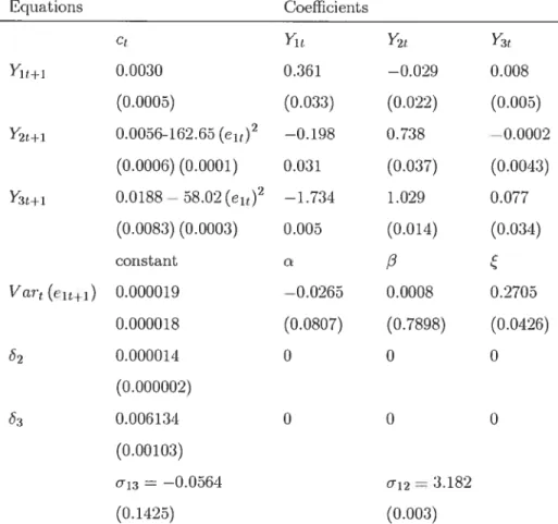
1.1 Estiinatecl resuits of the Factor CARCII in mean (see Bekaert and Lin (2001)) 45
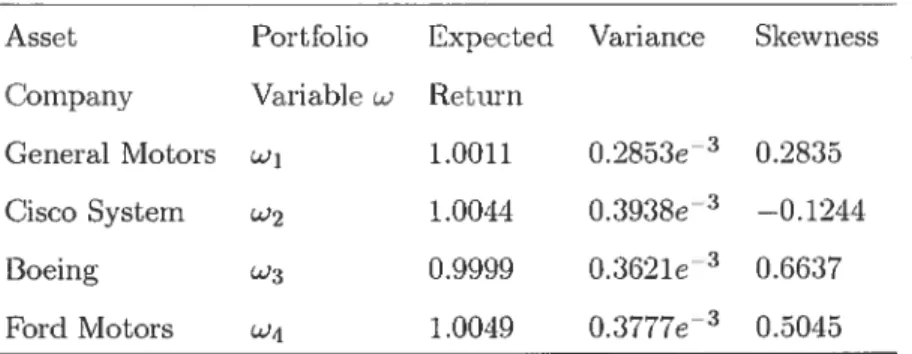
2.1 Asset company return moments 87
List of Figures
1.1 Price of coskewness: Price of coskewness inferred from simulated data according to the Factor GARCII in mean estimated in Bekaert and Lin (2001). IlS indicates the price of coskewness correspondingto Ilarvey and Siddiqne (2000) limit case. CLR indicates the price of coskewness corresponcbng to our formula 16 1.2 Price of squared net return: Frice of scinared net retnrn inferred from simnlated
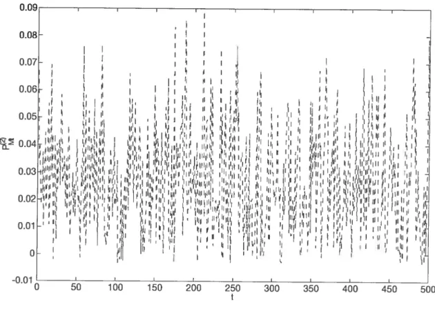
data according to the Factor GARC’lI in mean estimated in Bekaert and Lin (2004) 47 1.3 Risk preinium 011 the squared net returu: Risk preminrn on the sqnared net
retnrn inferred from simnlated data according to the Factor GARCII in mean esti
rnated in Bekaert and Lin (2004) 48
1.4 Quadratic SDF: Qnacfratic SDF inferred from simnlated data according to the Factor GARCII in mean estimated in Bekaert and Lin (2004). In the left hand side graph, we plot the pricing kernel rnc as a fnnction of I + 1 amirAft+1. In the riglit
hand sicle, we plot the average pricing kernel 49
1.5 Quadratic SDF: Fixing the price of the scinared market retuïn at the level 1.02. wliich in tnrns implies a thne varying ‘k’ we infer the qnadratic pricing kernel for
simnlated data accorifing to the Factor GARCII in mean estimated in Bekaert and Lin (2004). In the left hand side graph, we plot the pricing kernel mnu as a fnnction of t + 1 and rXfl1 = h the right hand side, we plot the average pricing kernel
50 2.1 SDF volatility surface frontier with a single excess returu: We nse onr
approach to imply a Mean-Standard Deviation-Cost Snrface for Stochastic Disconnt Factors nsing the excess simple retnrn of the Standard anci Poors 500 stock index over the commercial paper. Annnal US data, from 1889 to 1994. are nsed to compnte the SDF variance bonnd. The SDF feasible region is above this smtce 88
2.2 HJ frontier witli a single exccss return: We use the 11.1 approach to imply a Standard Deviation-Mean frontier for Stochastic Discount Factors using the excess simple return of the Standard and Foors 500stock index overthe commercial paper. Annual data from 1889 to 1991 are used to plot this frontier. The SDF feasible region is above this frontier
2.3 HJ Volatility Frontier: We implv a Mean-Standard Deviation frontier for Stochas tic Discount Factors using the return of the Standard and Foors 500 stock index and the commercial paper . Annual US data, from 1889 to 1994 are used to compute the IIJ variance bounci. The SDF feasible region is above this frontier. With CRRA preferences we vary exogenously the relative risk aversion coefficient and trace ont the resulting pricing kernels in this two—dimensional space. These pricing kernels are
represented by the points * 90
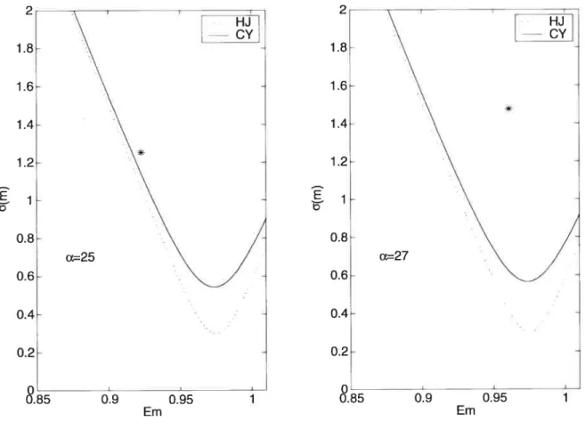
2.-1 SDF volatility frontier: IIJ represents the llansen anci Jagannathan volatility frontier and (Y represents oui volatility frontier. For each O:, we finci i = EmRf2)
and trace out the point (711. u (nï”’9 (771.ri))) in a two—dimeusional space. \Ve also
plot the point (Emt+i, u(mt+t)) where mt+] represents the SDF obtained in the
investor optiniization problem with CRRA preferences. We use tue return of the Standard and Poors 500 stock index over the commercial paper. Annual US data, from 1889 to 1994, are used to compute the SDF variance bound 91 2.5 SDF volatility frontier: IIJ represents the Ilansen and Jagannathan volatility
frontier and (Y i’epresents our volatility frontier. For each u. we finci îj EmR2
and trace ont the point (771,u(r7iT8 (117, ri))) in a two-dirnensional space. We also plot
the point (Ernt÷i,u(rn1.j)) where ru1y represents the SDF obtaineci with Epstein
and Zin (1989) state non—separable preferences. We use the retuin of the Stanctarci and Poors 500 stock index over the commercial paper. Annual US data. from 1889
2.6 SDF volatility frorrtier: IIJ represents the llansen arid Jagannathan volatility frontier anti CY represents oui volatility frontier. For each ci, we find = £mRt2
anti trace out
tue
point(.
u(,
77))) iii a twchmensional space. \Ve alSC) plot tue point (fmt+i, (m.i1))
where m1 represents tue $DF obtained with Gordon and S t-Amour (2000) state dependent preferences. We use the return on the Standard aiid Poors 500 stock index over the commercial paper. Anrntal US data. from 1889 to 1994. are used to compute the SDF variance bound 3 2.7 SDF volatility frontier: II] represents tue llansen anti Jagannatlian volatilityfrontier and CY represents oui volatility frontier. For each ci, we find î = EmRt2
and trace out the point
(,
u (rn7?(,
rj))) in a two-dimensional space. We also plot the point (Emt+j, u (mi)) where mt,+1 represents the SDF obtaineci with Melino anti Yang (2003) state dependent preferences with constant EIS, constant 4.and state ciepenclent CRRA. \Ve use the returrt of the Standarci and Poors 500 stock index over the commercial paper. Annual (8 data. from 1889 to 1991. are used to compute tlieSDF variance bound 94
2.8 Mean-Varimice-Cost (M-V-C) aiid Mean-Variaiyce-Skewness (M-V-S) sur faces: Given the portfolio menu, and sciuared portfolio cost, c. we solve problem (3.6) and plot in a three-clirnensional space the optimal portfolio (t’ ct,u(pmus)).
Then we vary exogenously [t and c and get the M-\ï-C surface. We then plot each optimal portfolio in a three-dimensional space: mean-standard deviation-skewness
(see the M-V-S surface) 95
2.9 Mean-Variance-Cost (M-V-C) and Mean-Variance-Skewness (M-V-S) sur faces: \Ve assume Coi’(mm. i’) = 0. Given the portfolio mean, p. ami scjuared
portfoïio cost, c, we solve problem (3.6) and plot in a three-dimensional space the optimal portfolio c*, u (ptr 8)). Then we
vary exogenously anti c anti get the M-V—C’ surface. We thereafter plot each optimal portfolio in a t.hree-dimensional space: mean-standard deviation-skewness (sec the M-V-S surface) 96
2.10 Mean-Variauce frontier: We first plot Markowitz Mean-Variance(M-V) portfolio frontier, then our Mean—Variance portfolio frontier (C’Y) for et =0.95 and 1 97
2.11 The residual price: For each portfolio pwhich helongs to the Mean-Variance-Cost
surface, Si, sec Figures 2.8 and2.9, we plot within Graph 1 the point (t’ Cou (m??L8,t’) ,ct) where [t, represents the portfolio mean, c is the cost of the squared portfolio re—
turn and Cou (mm v) is the covariance of the SDF with the residuals ohtained when regressing the squared portfolio on the portfolio itself. Graph 2 represents this covariance when the standard portfolio selection under skewness is used 98 3.1 Absolute Risk Aversion (ARA) and Pricing Kernel (PK) functions with
state dependence in fundainentals. The preference pararneters are:
fl
= 0.95,n = —5, p = —11. The regirne probabilities are: PH = 0.9, P00 = 0.6. For the
econornic fundamentals, the means of the consumption growth rate are =
(0.0015, —0.0009) , and the corresponding standard deviations = (0.0159, 0.0341). For the dividend rate, the parameters are py = (0,0) , = (0.02, 0.12). The
correlation coefficient bctween consumption and dividends is 0.6. The number of options useci is 50. The number of wealth states is n = 170. The left—hand panel
coutains the conffitional and rrnconffitioual PK functions across wealth states. EI’he right-hand panel contains the conditional and unconffitional ARA ftmctions across wealth states. The conditional ARA (PK) ftmction is the ARA (FK) furiction com puted within each regime. The uuconditional ARA (PK) frmction is the ARA (FK)
3.2 Absointe Risk Aversion (ARA) and Pricing Kernel (PIC) functions with state dependeuce in fundamentals: The preference pararneters are: = 0.95,
n’ = —5, p = —11. The reghne probabilities are: PH = 0.9 P00 = 0.6. For the
econornic fundarnentals, the means of the consnmption growth rate are btv =
(0.0015, —0.0009), anci the corresponcling standard deviations ux÷1 = (0.0159, 0.0341). For the cbvidend rate, the parameters are = (0,0) , = (0.02, 0.12). The
correlation coefficient between consumption and dividends is 0.6. The number of options nsed is 50. The number of wealth states is n = 170. The left-hand panel
contajns the nnconditional Ph ftrnction across wealth states for the Goodness-of-fit and the Ilansen and Jagannathan (1997) distance measures. The right-hand panel contains the unconcitional ARA function across wealth states for the Goodness of Fit and the llansen and Jagannathan (1997) distance measures. The rnwonditional ARA (Ph) fnnction is the ARA (Ph) ftmction compnted when regimes are not
observed 21
3.3 Absolute Risk Aversion (ARA) and Pricing Kernel (PK) functions with state dependence in preferences. The preference pararneters are
fi
= 0.97.(—7, —4.8), p = —10. The regime probabilities are Pli 0.9. P00 = 0.6. For the
econornic fnndamentals, the means of the consumption growth rate is [‘Xti = 0.018
and the standard deviations = 0.037. For the dilvidend rate Y4, the pa
rarneters are pF1 = —0.0018
, = 0.12. tf 1w correlation coefficient between consumption and dividend is 0.6. rfle number of options used is 50. The number of wealth states is n = 170. The left-hand panel contains the conditional and un
conditional Ph frmctions across wealth states. The right-hand panel contains the conditional and unconditional ARA fnrictions across wealth states. The conditional ARA (PIC) ftmction is 11w ARA (PIC) function compntecl within each regirne. The rnwonditional ARA (PIC) function is the ARA (Ph) function computeclwhen regirnes
3.1 Absointe Risk Aversion (ADA) and Pricing Kernel (PK) fnnctions with state dependence in preferences. The preference pararneters are 3 0.97,
n = (—7, —4.8), p = —10. The regirne probahilities are p» = 0.9, Poc = 0.6. For the
econornic fundamentals, the means of the consumption gTOWth rate is = 0.018
and the standard deviations uy, = 0.037. For the dividend rate the pa—
rameters are —0.0018 , 0.12. The correlation coefficient between consumption and dividend is 0.6. The number of options nsed is 50. The number of wealth states is n = 170. TI left—hand panel contains the unconchtional ARA
function across wealth states for the Goodness-of-fit and the llansen and Jagan
nathan (1997) distance measures. The rigl,t-hancl panel contains the unconditional ARA frmction across wealth states for the Goodness of Fit and the llansen and Ja
gannathan (1997) distance measures. The nnconditional ARA (Ph) function is the
ARA (Ph) ftmction conputed when regirnes are not observed 23 4.1 Trinomial Tree with a State Variable 18
A ma femme, Bignon. à mon père. Sarebou, à ma ,nère,Assanatou. et à mes frères et soeurs.
Remerciements
De nombreuses personnes et institutions sont à remercier dans l’accomplissement de cette thèse. Tont d’abord mes directeurs de recherche Eric Renault et René Garcia qui ont su orienter et guider mes recherches de manière fructueuse. Durant les aimées rie préparation de cette thèse, ils ont sn m’encourager et me prodiguer des conseils. Saris leur soutien, j’aurais stirement abandonné.
Je voudrais remercier mon cŒauteur Dietmar Leisen pour sa collaboration significative clans le deuxième essai de cette thèse. Ce dernier m’a beaucoup appris et je 1m suis très recomiaissant.
Je voudrais aussi remercier les nombreux organismes qui mont soutenu par leur financement: Centre Interuniversitaire de Recherche cri Analyse des Organisations (CIRANO), Centre Intcrnni versitairc dc Recherche en Économie Quantitative (CIREQ), MITACS (The Mathcmatics of Infor mation TcchnoloDr and Complcx Systems) et Ilydro-Qucbcc. Je voudrais également remercier la Banque du Canada pour son support dans la rédaction finale de cette thèse.
Je rouchais également remercier mon père Sarcbou. ma mère Assanatou, mes frères et soeurs. Boni, llassan, Samfi, Mansou, Rachi et mon épouse Bignorm de m’avoir non scrûernent enduré, mais encouragé et supporté clans les périodes les plus éprouvantes rie mes études.
Introduction générale
La validité des modèles d’évaluation d’actif financiers dépend de leur capacité à reproduire les caractéristiques des prix observés sur le marché. Sous certaines conditions dont celle d’absence d’opportunité d’arbitrage, Ilansen et Richard (1987) montrent qu’il existe un facteur d’actualisation aléatoire qui sert à évaluer le prix de tous actif financier. De part sa nature aléatoire, ce facteur est appelé facteur d’actualisation stochastique (SDE). Ilansen et Richard (1987) montrent que le prix d’un actif financier s’écrit corume la valeur espérée du produit du SDF et du gain de cet actif. La spécification de ce facteur dépend en général des hypothèses sur les préférences des investisseurs. La ligne directrice de cette thèse est l’étude parcimonieuse des différentes spécifications de ce SDF et leur implication en terme d’évaluation d’actifs financiers, de produits dérivés, de préférence et de choix de portefeuille.
Dans le premier essai de cette thèse, nous examinons comment l’équihbre d’un marché financier révèle, à la fois par les quantités détermes à l’équilibre et par les prix, les préférences des investis senrs pom’ trois types de caractéristique des rendements leur espérance. leur variance et leur asymétrie. Deux types d’approche sont utilisés pour cela. D’abord, en considérant une situation an voisinage de la non-incertitude (expansion en petit bruit), on calcule les demandes des agents pour différents types d’actifs risqués. L’idée est de considérer un actif en offre non nulle, représentatif du portefeuille de marché, et des actifs dérivés en offre nette nulle mais dont les gains sont des fonc tions non linéaires du portefeuille de marché. En faisant une expansion en petit bruit an premier ordre, on s’aperçoit que la demande d’actifs dérivés est déterminée uniquement par l’aversion des investisseurs pom’ la variance. Au niveau des prix, la rémunération du risque dépend du béta de marché connue dans un contexte moyerme—varianee (voir Markowitz (1952)). Le SDF impliqué par ce modèle est une fonction linéaire du rendement r[e marché. En d’autres termes une expansion en petit bruit au premier ordre produit le modèle d’évaluation d’actifs financiers CAPI\l. Toutefois, de nombreuses éturles empiriques ont souligné que cemodèle n’est pas pertinent en terme d’évaluation d’actifs financiers. Ce qui nous a conduit à faire une expansion en petit bruit au elenxième ordre. Dans ce cas, on s’aperçoit alors que la demande d’actifs diérivés est précisément justifiée par le
gofit des investisseurs pour l’asymétrie. Au niveau des prix, la rémunération du risque dépend non seulement du bèta de marché, comme dans un contexte moyenne—variance, mais aussi d’un coefficient de coasymétrie par rapport au marché. Le SDF impliqué par une expansion en petit bruit au deuxième ordre est une fonction quacfratique du rendement (le marché. Cette approche peut etre étendue à un marché à deux périodes où d’autres phenomuenes d’asymétrie doivent etre pris en compte dans la dépendance temporelle des rendements d’nne période à l’autre.
Une fois un facteur d’actualisation stochastique identifié, un des aspects importants est de le comparer à un SDE de référence pour s’assurer de sa pertinence ou de sa validité, Différentes méthodes sont proposées pour comparer les modèles d’évaluation d’actifs financiers, tester 1cm’ validité et s’assurer de leur pertinence. Bien souvent, ces méthodes utilisent cormne référence le SDF proposé par Flansen et Jagannathan (1991). Étant donné une série de rendements observés, Hansen et Jagannatban (1991) déterminent la variance minimale que doit avoir un SDF pour évaluer correctement les rendements d’actifs financiers, Le SDF (le Ilansen et Jagannathan (1991) (lépend des deux premiers moments des rcndements d’actifs financiers, donc ne prend pas en compte l’asymétrie observée dans ces rendements, Pom’ les actifs fondamentaux comme les indices boursiers et les indices obligataires qui servent à l’évaluation des modèles, les moments d’ordre supérieur à deux ne jouent pas en général un rôle déterminant. Toutefois, dans plusiem’s études empiriques, il est admis que ces deux premiers moments ne caractérisent pas entièrement la distribution des rendements, Un (les faits stylisés est que la distribution des rendements est souvent asymétrique. Comme nous l’avons précisé dans le premier chapitre, l’asymétrie peut s’avérer importante pour la prise de décisions d’investissement. D’abord, un investissement avec une distribution de cash—flows fortement etalce a droite peut etre attractif meme si son ratio de Sharpe n’est pas tres eleve. Ensuite, les contrats d’option d’achat ou de vente exhibent evidemment (les payoffs tres assyrnetriques. Pour toutes (‘es raisons, la frontiere proposee par llansen et Jagannathan (1991) dans le plan moyeene variance pour decrire les SDF admissibles ne met sans doute pas assez l’accent sur la remuneration (le l’assvmetrie.
SDF qui évaluent correctement nonseulement les rendements d’actifs financiers fonclamentanLx mais aussi ceux de produits dérivés et de stratégies financières complexes telles qne celles utilisées par les fonds spéculatifs. Nous supposous que le gain de tout produit dérivé peut être approximé par nue fonction quachatique des actifs primitifs. Intuitivement, nous augmentons l’ensemble des oppor tunités d’investissement des agents économiques en considérant non seulenient les actifs financiers mais aussi les produits dérivés qui sont fonction des actifs primitifs. Tout connue le SDF de Ilansen et Jagannathan (1991), ce SDF est simple et facile à utiliser, il peut être utilisé pour coiuparer les modèles d’évaluation d’actifs fmanciers et pour tester leur validité. Il peut être interprété comme nue simple extension du SDF de Ilansen et Jagannathan (1991). Toutefois, sa particularité est qu’il prend eu compte les moments d’ordres supérieurs des rendements d’actifs, en particulier l’asymétrie observée dans ces rendements. Le SDF proposé dans cet essai est une fonction quadratique des rendements d’actifs primitifs. Récemment, de nombreux auteurs parmi lesquels Harvey et Sidcbque (2000) et Barone-Adesi et al. (2001) ont souligné l’importance d’utiliser un SDF qui est une fonc tion quadraticue du rendement de marché pour étudier l’impact de l’asymétrie sur les rendements espérés d’actifs financiers. Par exemple, Ilarvey et Siddllque (2000) montrent qu’un SDF fonction quadratique du rendement de marché permet d’expliquer les variations en coupe transversale des rendements espérés entre différents actifs. Tout comme le SDF de Ilansen et Jagannathan (1991). nous montrons que le SDF proposé dans cet essai peut être interprété en terme de choix de porte feuille en proposant une simple approche de choix de portefeuille sous asymétrie. Cette approche est une simple extension de l’approche moyenne-variance (voir Markowitz (1952)) et de l’approche moyenne-variance-asymétrie (voir de Athayde et Flores (2004)). Cette dernière approche consiste à chercher le portefeuille le moins risqué
(
portefeuille ayant la plus petite variance) parmi tous les portefeuilles ayant un même coefficient d’asymétrie et une même valeur espérée. En terme de choix de portefeuille, cet essai apporte deux contributions. Premièrement, nous généralisons le problème de choix rie portefeuille résolu par de Athayde et Flores (2004). DenLxièmemnemit, nous proposomis mie approche simple qui permet de déduire facilement (sans une résolution numérique) la solution à ce problème.Dans une première application empirique, nous illustrons la perte d’information sur le SDF qni résulte d’une utilisation du SDF de Ilansen et Jagannathan (1991) lorscin’il y acte forte présomptions que l’asymétrie est évaluée sur le marché. Dans une ctemdème application empiridlue, nons utilisons le SDF proposé dans cet essai ponr vérifier si les modèles basés sur la consommation explicnent ou non l’énigme de la prime de risque mise en évidence par Mehra et Prescott (1985). Le SDF proposé dans ce essai rend l’énigme de la prime de risque encore plus difficile à expliquer. Dans une troisième application empirique nons montrons que les investisseurs qui ont une préférence pour l’asymétrie choisissent un portefeuille autre que celui proposé dans de Athayde et Flores (2004). fls ne choisissent le portefeuille proposé par de Athayde et Flores (2001) que sons des hypothèses plus restrictives qui ne sont en général pas vérifiées empiriquement.
Dans le troisième essai, nous présentons un modèle économique avec changements de régime qui produit et explique les énigmes de l’aversion pour le risque et du SDF mises en évidence dans Jackwerth (2900). En résolvant le problème de choix de portefeuille de l’agent économique on s’aperçoit que le SDF peut étre interprété connue un taux marginal de substitution intertemn— porel. En admettant que la fonction d’utilité de l’agent économique est concave (pour mi agent économique averse au risque), le taux marginal de substitution intertemporel doit etre une fonc tion décroissante de la richesse de l’agent économique, tout comme d’ailleurs la fonction d’aversion absolue pour le risque de l’agent économique doit également étre une fonction décroissante de sa richesse. Toutefois, les études empiriques (voir Jackmverth (2000) et Ait Sahalia et Lo (2000)) mon trent que ni le SDF, ni la fonction d’aversion absolue pour le risque n’apparaissent cornue des fonctions décroissantes de la richesse. Pour expliquer ce paradoxe, nous construisons un modèle où les préférences des investisseurs et leur consommation dépendent d’une variable d’état qui suit mm processus de type Markovien à deux états et simumilons les prix d’options d’achat européennes. En utilisant la méthodologie proposée par Jackwerth (2090), nous déduisons la fonction d’aversion absolue pour le risque et le SDF pour chaque valeur de la richesse. Ces fonctions présentent les memes énigmues que celles observées par Jackwerth (2000) et Ait Sahalia et Lo (2000). Lorsque nous appliquons la mnéme méthodologie dans chaque état de l’économie, l’énigme de l’aversion absolue
ponr le risque disparait. Nos résultats suggèrent que ce modèle rationalise et explique l’énigme (le l’aversion pour le risque et du SDF mises en évidence par Jackwerth (2000).
Dans le quatrième cbapitre, nous présentons nn modèle d’évaluation des produits dérivés par la méthode d’arbre lorsque le processus du prix du sous—jacent est affecté par une variable d’état non observable. Dans un modèle (le marché à une période, nous montrons (iie ce modèle est observationnellement équivaleut an modèle proposé dans Boyle (1988). Sur deux périodes, nous montrons que ce modèle généralise le modèle (le Bole (1988). Dans ce modèle, la variable (l’état non observablecapture les faits marquants mis en évidence par l’observation des prix d’options, en particulier l’asymétrie et la dynamuique (le l’asymétrie présentes dans les actifs dérivés.
Cliapter Ï
I1i1i)ÏicatiOlis
of
Asynimetry
Risk
for PortfoÏio Analysis
aiid Asset Pricing
Asynunetric shocks are common on rnarkets and will lead to payoffs that are iiot norrnally cistrihiited anci exhibit skewness. Moreover, even when the primitive assets have symmetric payoffs, typical derivative assets display a high degree of skewness. The risk-returrr trade off on such payoffs may not be captured well by mean-variance analysis. llowever, Samuelson (1970) arguecl that mean-variance analysis is stiil a valid approach to characterize the optimal portfolio problem in general, i.e. even in those cases when the decisiou maker has a general concave von Neurnan Morgenstern utility function and asset returns are not normally distributed. lus resuit is basecl on the liinit of portfolio holdings under infinitesimal risk. We argue, in the presence of “small” risks h is necessary to study also the siope of portfolio holdings in the neighborhood of zero risk, and thereby incorporate skewness risk into the analysis. This paper extends Samuelson’s analysis of frnancial decision making to derive agents’ portfolio holdings and the equilihriunn allocation under mean-vari ance-skcwness risk.
We characterize portfolio holdings using risk—tolerance anci a terrn we cali skew-tolerance which contains the third derivative of an agents utility function. Risk—tolerance captures the mean— variance trade-off and skew-tolerance the mean-variance-skewness tracle-off. Using appropriately defined “average” risk-tolerance and “average” skew-tolerance weshowthat such an “average” agent
sets prices whule cadi heterogeneous agent’s holdings are proportional to the difference between the agents skew-tolerance and that of the “average” agent. The proportionality factor is cleterrnined through co-skewness with the market; two—fund separation theorems typically do not hold under skewness risk. A relateci work is Judd and Guu (2001) where Samuelson’s analysis is also extencteci to an asyrnptotically valid theory for the trade-off between one risky asset and the riskless asset in single perioci setups. Ilowever, while their approacli is baseci on bifurcation theory. oui results are based ffirectly on limits of fn’st orcler conditions.
Our paper makes the foilowing contributions
First, we generalize Sanutclsons analysis by not irnposirg that risk premia are Iocally propor tional to variance. By relaxing tIns restriction, we are able to characterize the price of skewness in
risk. it reniains true that am- risk is compensateci onlv tlwoiigh its relationship wit.li the market. either through the standarc[ market beta or through market co—skewriess which is akin to a beLa with respect to the squarecl rnarket return. In this respect, one may say that neitirer idiosucratic variance nor ichosyncratic skewness are compensatect iii ecinilibrium. We thereby provicte a foun dation for empiuica.1 stuclies tha.t exLend the CAPI\1 model using in an ac[-lioc vay the scluared market return as a second factor. Furthermore this paper provides a methoci to cteterïnine portfolio holdings uiider skewness ri sk.
Second, we study extensively the pricing implications of a Stochastic Discount Factor
(
SDF) specification that is cluadratic with respect to market return. Although motivated by the above small risk analvsis à la Samuelson (1970), this stucty h valid under very general settings and can be comparecl to previous litemature on the pricirig implications of skewness risks. \‘Ve revisit beta pricing mider skewness as alreadv considered b Kraus and Litzenberger (1976). Barone-Actesi (1985), Harvey and Sicktic1te (200tJ), Dittmar (2002), and Barone-Adesi. [rga anct Gagliardini (2004) amo;ig others. For the purpose of derivative asset pricing, we also relate skewness pricing to risk neutral variance(
Rosenberg(2000)) and price of volatility contracts(
Bakshi anci Madan (2000)). We shed more light on beta pricing relationships as proposeci by Ilarvey and Siddique (2000) by showing that they correspond to a. lirnit case which is strictlv speaking a.t odds with a no—arbitrage reciuirement, narnely the case of a zero risk—neutral variance of the market. We put forward a more general beLa pricing relationship which explicitly depencis on the price of the sciuared return on the mnarket portfolio, or ecpmivalently, on the market risk neutral variance.Finally, while the statistical identification of a signiflcantly positive skewness prernmm is gener— allv considerect to be a chfficult task (Barone_Adesi, Frga and Gagliardini (2001)). we provicle some empirical evidence whicli suggests that such premia show up in a more manifest way when the are comrsiclered from a conclitional point of view. This evictence is documenteci froin sinuilated data calibrated on the GARCIT factor model with in urean effects recently estimateci by Bekaert and Liu(2004). i\/Ioreover, this empirical evideirce also shows that neglecting the market risk neutral
variance as Ilarvey and Siddique (2000) beta pricing inodel does lead to a severe underestimation of tbe skewness premium which may go so far as to invert iLs sign.
The remainder of the paper is organized as follows: the next section discusses portfolio choice and asset pricing in the context of infinitesimal risks. Section 3 studiles quadratic pricing kernels in the conditional setup of Ilansen and Richard (1987). Section 4 makes an ernpirical assessment of the order of magnitude of the various effects put forward in section 3. Ail proofs are postponed to the appendix.
2.
Static Portfolio Analysis in Terms of Mean, Variance and Skew
ness
Samuelson (1970) argues that, for risks that are infinitely small, optimal shares of wealth invested in each secnrity coincide with those of a rnean-variance optirnizing agent. llowever Samuelson (1970) also derives a more general theorem about higher order approximations. To further characterize the way the optimal shares vary locally in tbe direction of any risk, that is their flrst derivatives at the limit point of zero risk, one needs to push one step further the Taylor expansion of the utility function; carrying this out will lead us to n mean-variance-skewness approach.
We start here from a slight generalization of Sarnuelson’s approximation theorem. Following closely his exposition, let us denote respectively by Ri, i = 1, ...n, the retm’n from investing $1 in
each of security i=1,...n. The random vector R (Ri)1<< defines the joint probability distribution of interest, which is specified hy the following decomposition:
R (u) = i+ u2a (u) + uY. (2.1)
Ilere, a (u), j = 1, ...n, are positive ftmctions of u and p. is the gross return on the riskless (safe) security. The u parameter characterizes the scale of risk that is crucial for our aualysis. We are typically interested in this section in local approximations in the neighborhood of u = 0. The small
Hoise expansion (2.1) provides a convenient framework to analyze portfolio holdings and resulting equilibrimu allocations for a given random vector Y = (Y)1< with E [Y] = 0, and Var (Y) = Z
a symrnetric and positive definite rnatrix1.
In equation (2.1), the terrn u2a (u) has flic interpretation of the risk premium. Samuelson (1970) restricts the hinction a (u) to constants; nncler this assnmption risk premia are proportional to the squared scale of risk; we relax this restriction throughout since it would prevent us from
analyzing the price of skewness in equilibrium. Throughout we refer to a (u) (a (u))1_1 as fie vector of risk premia.
2.1 The individual investor problem
XVe consider an investor with Von Neuxnann—Morgenstern preferences, i.e. she clerives utility from date 1 wealth according to the expectation over some increasing and concave function u evalnated over date 1 wealth; for given risk-level u she then seeks to determine portfobo holdings (w)1<<
e
r of risky assets that maximize lier expected utility.max
rpn Eu +
Z
w (R (u)—ri)) (2.2)
(w)1<<L
i
Note that for the sake of notational simplicit the initial invested wealth is normalized to one. The solution of this prograni is denoted by (w (u))1<i<n artd depends on die given scale of the risk u.
Tire cjnestion we ask is then the following: to what extent does a rfaylor approximation of u allow us to understand well the local hehavior of tire shares w (u), i = 1,.. n, in tire neighborhood of zero risk. u = 0, that is to correctly characterize the two quantities:
w (0) = lim w (u) and (0) lin (u) (2.3)
for i=1...n? Samuelson (1970) stresses that a tffird-order Taylor expansion of u is needed to do the job. We slightly extend his result hy showing that its remains valid even thougb tire function a (u) are not assurned to be constant.2 Let us then consider a third orcler Taylor expansion of u in tire
1Sarnuelsori (1970) provides a heuristic explanation of (2.1) that is of interest for reaclers accustomed to contrnuous time finance models; he couches this ternis of Brownian motion of time and identifiesu with the square root of Mmc. 2Let W(u) n w(R(u)—n) denote end of period wealth and note that W (0) p. For the sake of
neighborhood of the safe return i: u, (W) =
()
+‘(p) (W — t) + 2! (W — )2 + U (W — )3 (2.1)Let us clenote by
(
(u))1<< the solution of the approximateci problem:max Eu* (rt+Êwi(Ri(u)_)) (2.5)
(W)i<j<u
i=i
(O) and ‘ (O), i=1...n are deffied accorclingly by continuity extension as in (2.3). We prove:
Theorem 2.1 Under suitabte smoothness and concavity assumptions. tue sotution b [lie gene rat probiem (2.2) is retated asyinptoticatty to that of [lie 3-moment probtem (2.5) by the tangency
equivatei ces:
=
(O) = (O) for ail i=i,...,n.
This theorein states that third—order Taylor expansions give tangency eciuivalence. The intuition behind this result is:
1. The optimal shares ofwealth invested wj (O), i=O,...n, in the lirnit case u O depend only on its first two derivatives u’ (ji) and u” (p). Thirs a second order Taylor expansion of’u, that is a mean-variance approach, provides a correct characterization of these shares.
2. The flrst derivatives with respect to u,
4
(O) i=1,...,n of optimal shares, in the ilmit case u O, depenci on the utility function u only through its first three derivatives u’(ii), u”()
and u” (p). Thnis a third order Taylor expansion of u, that is a rnean-variance-skewness approach, does the job.As far as optimal shares are concerned, theorem 2.2 below confirms that they are conformable to standard mean—variance formulas, that is formulas iisually oht.ained with an assmnptiori of joint normality of returns:
Theorem 2.2 Tue veci or w (O) = (wj (0))-< ofshares of weolih invcsted in the tirnil case o- = O
is given by:
w(O) = TL1a(O).
wheTe ci(O) = (a ())<< is the vector of jisÏ,- and T =
—
fl() is the risk toierance coefficient.
To see
tue
equivalence with standard fountulas commonly deriveci uiuler an assumption of joint norrnality, two remarks are in order:1. While joint normality with a general utility ftmction would lead to introduce a kind of average risk tolerance coefficient (—Eu’ (W) /Eu” (W)) with W = w (R — tt), this actually coincides with T in the lirnit case u • O.
2. Joint normality would iinplv. in ecimÏibriuiti. constant functions a (u) (sec theorent 2.1 below). In sucli a case, the formula of theorem 2.2 cnn be rewritten:
w (O) T(VarR(u))1 u2a.
where u2a ctefines the vector of risk prernia.
Generally spealing, following theorem 2.2, if we see optimal shares of wealth invested w (u) as ecluivalent to T1a(u) in the neighborhood of u = O, we get a Sharpe ratio for optimal portfolios
ecluivalent to:
E{wT (u) (R (u) -[t)]
—uP (O) (Var [w’ (u) R (u)])
where
P (O) = [ci’ (O) (O)] (2.6)
clenotes, by unit of scaling risk u, the potential performance of the set R of returns as in traclitional mean variance analvsis [sec e.g. Jobson arid Korkie (1982)]. 0f course, the above analvsis neglects
the variation in eciuilibrimn of the risk prernium functions a (u). We are going to sec in theorem 2.1 helow that these furictions will not lie constant, even locally in the neghborliood of u O, as soon as asset return joint probahulity distribution features some asymmetries.
These asymrnetries will actually play a double role in the local behavior of optimal shares of wealth invested. First, preferences for skewness woulcl increase, ceteris paribus, asset fiemands in the direction of positive skewness. Second, rnarket eciuilibriuin induced variations in risk prernium which potentially crase this eflèct. To sec this, let us clefine the co-skewness of asset k in portfolio
as:
Defiuiitioii 2.3 The co-skewness of asset k in portfolio is:
CL.
Goy
(‘
T2) =(2.7) Var [Y]
where Th. = E [YYYJ is flic 7atrix of couariances between Y ami cross prodnct YY;, i.j=1 n.
Wc will sec in section 3 lielow that this notion of co—skewness is tiglïtly relateci to a measure put forwarcl by Kraus anci Litzenberger (1976) (sec also Ingersoll (1987), p 100). For the optimal portfolio ‘(0) characterized in theorem 2.2, we have CL. (‘(0)) CL. ctefinecl as:
ck p2(0)aî(0)ZFLZ ‘a(O). (2.8)
Typically, asyrnmetry in the joint probability distribution of the vector R of returns means that at least sorne niatrices F, k=1 n are non-zero. We get the following result:
Theorem 2.4 The stope‘ (0) of the vector (0) of optimal shares of wealtk inuested in the neigk
borhood of u O s gven by.
(0) = T’ [a’ (0) + pP2 (0) c]
wkere a’ (0) (a(0)) is tue oector of marginal ïsk premia. c = (ck)i<k<fl defined by (2.8)
In other words, up to variations o’ (0) of risk preniiruus in equiiibriuiti, a positive co—skewriess
of asset k xviii have a positive effect ou the demand of this asset. This positive eftect xviii be ail the more pronounced that the skew tolerance coefficient p is large. 0f course, this interpretation is based on two irnplicitly maintaineci assumptions:
1. The slcew tolerance coefficient is nonnegative (! > 0). TIns assumption conforms to bot.h the literature 011 prudence [Kimbail (1990)] antI the literature on prefèrences for high order moments [Dittmar (2002), Ilarvey anci $iddique (2000), Ingersoll (1987)]
2. The vector e
()
(Ck (W))1<k<fl represents a mriltivariate notion of skewness that investors do like to get positive, cornponentwise. This assertion is justified bv the fact that on average:n E [(—Y)3]
Var[IY]
is positive if and orfly if the portfolio return is positively skewed. 0f course, individual
preferences for positive skewness xviii increase. ceteris paribus. the ecjuilibriuni price of assets witli positively skewed returns. TIns xviii actually appear in the eciuilibrium value ci’ (0) of risk premium siopes in the neighborhood of u= 0.
2.2 Equilibrium allocations and prices
Let us consider consider asset markets for risky assets i=1,2,...,n with agents s=1,...,S. Eacli agent
is characterized by a Von Neumann-Morgenstern utility firnctions u3 and associated preference
coefficients:
u (pc) T U
@)
T3 = — ,, ami p =
‘u3 (ht) 2 u3(t’)
Note tliat for the sake of notationai simplicity, we assume that the net supply of each riskv asset i=1 n is exogeneous and fixed to unitv as a normalization. Then, in the limit case u 0. the inarket clearing conditions can be written:
(2.9)
where (s) (0) = (j
(°))1<j< and e clenotes the n—clirnensional colurnn vector, the componerits of
which are ail equal to 1. Beiow, it vill be coiwenient to corisicler arr average investor characterized by average holdings , an average risk tolerance and average skew tolerance, where
s s p3T5 rrC =-T3, (2.10) s1
Z
-r5 sj—1if ail individual were identical, each one would buy the average portfolio Z5. The link between the two average preference coefficients anci and individual portfolios clemands is characterized h theorern 2.5.
Theorein 2.5 In equitibrium, in tire timit case u 0, tire opti7 at si ares of weatth invested (u) by agents s = 1 S is characterized by:
() (0) ,(s)’(0)
= T3[p3 — P2 (0) -1c() for s=i S.
where p2 (0) is tire (sqnared,) market Sharpe ratio and e
()
is tire vector of tire rnarket co-skewness coefficients.In other words, in the limit case u 0, the vector (s)(u) of optimal shares of wealth invested is as in n standard mean-variance separation theorem. All individuals buy n share of the market portfolio e the size of this share being determined by the comparison of individual risk tolerance
T3 with respect to average one. Freferences for skewness oiily piay a role for the siopes (s)’ (0) of
the shares of wealth invested in the ueighborhoocl of zero. A positive rnarket co-skewness ck
()
will have a positive effect on the inctividual s demand of asset k if and oiily if his skew tolerance coefficient is niore than the average one . On the contrary, if p3 <, the positive effect of asset k co—skewness on its market price is higher than rectuirecl to coinpensate the investor’s preference for skewness.In order to characterize the asset pricing implications of risk tolerance and preference for skew ness, we deduce the local behavior of the risk premium in eqiiilibrium:
Theoreiri 2.6 In [ha iinifl case u 0. the equilibiinin. risk prenuam uector u (u) is such [liai ihe average portfolio is optimal for [ha averaqe inuestor:
1a(0)
aitd us stope in [ha neughborhood of zero 15 given by:
a’(O) -P2(0)c().
where P2 (U) JTL is the (squtared) marÏuet Shaipe ratio and c() is the vector of [ha marluet
co-skewness coefficients.
Note that, by comparison of theorems 2.4 arid 2.6, the eciuilihrium siopes are precisely such that the average agent wouM have no motive to deviate from the rnarket portfolio (‘ (0) 0 for
tue average jnvestor)
Theorem 2.6 gives as a new asset pricing model. While approxirnating risk preiriia by their
limit va’ues a (0) would dearlv give the Sharpe—Lintuer CAPI\I, approximat)ng them by liiglier orcler expansions n (0) + ua (0) gives a new rnean—variance-skewness asset pricing model. A con venient way to describe the implications of an asset pricing model is to characterize it through a
Stochastic Discount factor (henceforth SDF), see e.g Cochrane (2001). By definition. a $Df ‘ru (u) must. be ahie to price correctly ail available securities; here we therefore need: Em (u) = and
E [in (u) (i + u2a (u) + u)] = 1 for i=i n. We ctenote R.1 (u) = (u) the market retm’n.
\Ve are then able to translate theorem 2.6 in terms of a SDf:
Theorem 2.7 The random variabte:
in(u) =
±
— (u)— ERM (u)) + -—2 [(RAI (u) — ERA,J (u))2 — E (RAI (u) — ERA]
(u))2]
/t /iT T
is u SDF consistent with variance-skewuess risk premivin defined hy u (u) = u (0) + ua’ (0) where
a(0) and a. (0) are given hy theoiem 2.6.
The conjunction of theorems 2.6 anct 2.7 summarizes what we have learnt so far about portfolio
1. Due to heterogeneity in preferences for skewness, the common two-fund C’APM separation theorem is violateci: diffèrent individuals rnay hold in equilibrium different risky portfolios.
2. Ilowever, the pricing implications of a cormnon separation theorem remain truc iii some
respect. Somewhat nnexpectedly, the market retnrn alone is still able to smnrnarize the pricing of risk. 0f course, siuce not only market betas but also market cŒskewness must be taken into acconut, both the actual market return and its squared value enter liuearly in the pricing kernel.
Following the serninal paper by Kraus auJ Litzenberger (1976), Ilarvey and Siddique (2000) auJ Dittmar (2002) among others have recently stuffied the empirical implications of a SDF which involves a qnadratic ftmction of market return. Theorem 2.7 above provides a theoretical basis for doing so. Section 3 will elaborate more on the pricing implications of such a SDF.
3.
Nonlinear Pricing Kernels
The pricing implications of a SDF’ formula tbat h quacfratic with respect to the market retmn are stndied in this section, first with a linear beta pricing point of view auJ second in terms of derivative pricing.
3.1 Beta pricing
hi their paper about conclitional skewness in asset pricing tests, Ilarvey and Siddique (2000) start with the mnaintained assumption that the SDF is ciuadratic in the market retnrn:
= vot + !JflRj +v2tRj+1. (3.11)
It actually suffices to revisit onr section 2 ahove with a conditional viewpoint to sec theorem 2.7 as a theoretical justification of (3.11). lien, the coefficients VOt, Vit and V2f are ftmctions of the
From t.heorem 2.7. ‘e interpret the facIors coefficients as: p 112t = > ° (.3.12) T and 1 vit = ———— — <0. (3.1:3) /I)T [I5 T
It is worth characterizing the role of the two factors RMt+i and in the SDF (3.11) in Lerms of beLa pricing relationships. Assuming the existence of a conditionali risk—free asset (with returu fit), we can write for the net excess return ri — fit of any asset :
E [ij,+irflt+i] 0,
that is:
1E [riti] + vtCovt [‘rt+i. R111,+11 + i’2CO [rit+I. R11] = O
or, using the market net excess return. we get:
±Et [r+] + (Vit +2[ttV2t)Coet [rit+i.iit+t] + v2tCout [rit+ ‘Iti] = 0.
that is:
E [r+] itCon[Tjt±1, TMiJ — À2Coe [7t+i,
with:
/\yj = —[tt(Vit +2ftt121) anti /\2t = Pt1’2t.
if Vit anti v2 are interpreted in tenus of preferences of an average investot as in (3.12) anti (3.13),
we deduce:
1 )—
= + (E,R+ —i’) and À2t
Note that ‘\2t is something like a structural invariant. orilv tirne varying through the value of
he non—negative and ail the more positive that preference for skewness is high. $irniiariy, Ài is expecteci to be positive anci time varying insofar as the market risk prentium (EIRAII+1 —t) is.
To summarize:
Theorem 3.1 Under the maintained ussurnption (3.11) of a quadratic $DF, net etpected ret urus are given by:
Etrj÷i = À1Cov [rjt+i,TAit+1] — À2Cuv. [rit+i,
rit+ïÏ
1 in addition, theorem 2.7 appties, and À2t are 11017 negative. ‘\21 = is dci ermined by
average preferences for skewness while:
À11 = +2/\2IEITML+l.
Note that ‘\lt lias two components which are both increasing with the average risk aversion,
first as 1/T and second as the rnarket risk premiu;n Etri1jt+i. \Vhen applying theorem 3.1 to the market return itseif (rti = rM(
),
we get even more insight 01 what inakes /\jt large:Corollary 3.2 Under flic assumptions of t.heorem 3. 1
EITMt+i Shewt(TA[t+1)
VartrArt+l t7artr,iti where 5’kew (rMt+1) =
Guet
(rAIt+1,’rt+l)In particuiar, we can see that theorem 3.1 coincides with the standard Sharpe-Lintner CAPM formula when À21 = 0, that is the average preference for skewness is zero. By contrast, À1 is
augmented in the general case by an additive term which is proportionai to both À21 and
Ske71.(rMt÷1) = Cue1 (rAIt+i, r,jtii) = Etrrt+t (EtrMtil) (Etrit+i)
This notion of market co-skewness lias aiready been put forwarcl by IIarvey anci Sicldic1lte (2000) anci theorem 3.1 arid corollary 3.2 correspond to their formulas (7). It is also worth rewriting the pricing relationship of theorem 3.1 ancl corollary 3.2 in term of betas:
G
and
r. _fr. t) t ir .2 ( 2 t (t
U1? it+1 — tt’AItfI)jtj — 211’ alttMl-j-1 t’)imt — fmrnhirtttI
‘ k’ ‘-‘i
Cour [rtti ,r&l t . .
where t3im( = 15 the standard market beLa whale the beta coefficient with respect to
Covt[rt+i.r 1
the sqnared market return: 7jmf
= var r2
Mt+1 is tightly related to tlw nieasure ol co-skewness Att-’-l
afreadv introduced in section 2. More preciseh it is straightforward to sec tint the retuin decom— position of section 2 gives: 7t = cfr (u) with c7 (0) as introduced in definitioii 2.3. \Vhlle we
had aheacly seen in theorem 2.6 that risk premirnus in equilibrium where influenced b- skewness preferences in proportion of the vector c
()
of market cŒskewness coefficients, the same vector shows np in the beta pricing relationship (3.14) with 7jmj = (u). Note that what Ilarveyand Siddic1ue (2000) eau “market co—skewness” is actually Skew1(rAj1) = 7rnntt (Vartr1t+1).
11w beta pricing model (3.14) with a second beta coefficient interpreted in terms of co-skewness with the market is chserx’ationallv equivalent to a conditional version of the three—moments C’AFM fnst proposcd 1w Krans and Litzenberger (1976) (sec also Ingersoll (1987),
plOO).
Whule they pnt fonvard a rneasnre of co—skewness defined as:c,
(Rj1+1 — ERI1+l)2) biint =Cov1 (RAJf÷i (RAftti — ER[t+l)2)
we have preferred to remain truc to a genuine notion of beta coefficient as y,-. Flowever, the difference between the two is just a matter of normalization and is inmiaterial in terms of asset pricing. In particular (3.15) enhances as formula (61) in Ingersoll (1987) that tbe beta pricirig relationship differs from Sharpe-Lintner CAPM by a factor proportional to the difference between the two betas. It is however worth noticing that these authors derive this pricing relationship by using a ntility function directlv defined over mean, standard deviation and skewness. The srnall noise expansion approach of section 2 affords more tbeoretical nnderpinnings for doing so.
Normalization in terms of beta coefficient is usually convenient since it allows a direct interpre— tation of beta loaffings in terms of factor risk premium. For instance, when À2, = 0, (3.11) applied
to the markeL gives the nsual formula: /\it = with
(l) — 1t”Mt1-1 Mi — y aiî5
It is. however, worth noticing that in general case, À1 aiid À21 cari not be reaci as simple risk preniimn associated respectively to the two payoffs r511•1 and iti• Even if we assmne that does correspond to a payoff of a portfolio available in the market with price the risk premium011 sucli a payoff:
-p
()
lit(r1)2 (3.16)will not coincicle with (—À2t7)t). The difference comes from the fact that the two factors are not orthogonal. À1 does clepenci on À2t (sec corollary 3.2) and the expression of À2t in frmnction of the
ecluilibrium prices is more involved:
Theoreiri 3.3 Ifri = E [mt+irtt+i] denotes the equitibrinin price of apayoffr1,1 tue have:
Ymrnr1 -
(ru)
À2=
2 2
1
—flt (r5It÷1.H+[)
where accoïding b (3.16), P (rit) is the riskpremium on the asset wzthpaYOffTEl and p (rAp1,
deno tes the square (conditionat,) tinear cor7viation coefficient between r111 and
L÷
i.It is worth considering the limit case when r11 is almost worthless. From (3.16):
(2) 2
lim (rit) = EtrAIH1 (3.17)
tjO rit Vart (r1+1) 11m this limit case, one gets:
(1) E1r111
Yrfl ml 511 — Car1(r2
Alt--1
“21— 1 21. .2
—Pt
]
wt-i, ‘w,i-iwhich actually coincides with the fonriula put forward by Ilarvev and Sicldiciue (2000). Ilowever, tus lirnit case appears to he at odds with a no—arbritage condition sirice g1 = E [înt+irrnti]
should be positive. Incleecl, as shown in subsection 3.2 helow, o- = r11t11 mnay be interpreteci as
Besicles the no—arbitrage condition, the fact that risk neutral variance is significantly positive is of conrse an empirical question. Since, from (3.16):
p(2)
()
— — (‘3 19) — Var1 (ri1+i) — *2one may expect that considenng the hmit case (3.11), that is = O leads to overestimate
and then to nnclerestimate À21. The relevant einpirical issue (sec section 4) is then to decide if considering only the limit case (3.18) leads to an economically siguificant nnderestimation of the weight À21 of coskewness in the two factors pricing relationship (3.15). If ii is the case, wc must realize tbat À21 actually depends on investors preferences for skewness as they show np eithcr in the (rnarket) price of squared market return or, equivalently, in the risk neutral variance of the market return.
3.2 Derivative pricing
The huge expansion of derivative asset markets, introclucing asset payoffs which are uonllnear ancl often skewed functions of uuclerlying primitive asset returns, has motivateci the renewal of iuterest in asset payoffs skewness. For salie of notational simplicity, we consider in this subsection orily options written on the market return. Ilowever, most of
tue
results could be extendeci to other primitive assets. Let us then consider the pricing issue for a payoff h1(.)
of the market retuin, the definition of which may depend on conffitioning information. Maiutaining, as we do in this section, the as sumptiou that a valid SDF is quadratic meaus that the price of the payoff lit(Rpj1+i) coincides with the price of its (conditional) affine reçession h2 (RAII+i) = DL1 [lit (RMItI) RA[t+i, R,11+1] ouRAJt+1 and
r
(L2)E. [rnt+iht(RA,I,+i)] = E1, [mt+1h1 (Rr1+)
Besicles this, uuderstanffing why a C’AFIVI Sharpe-Lintuer pricing does not accommodate well the pricing of derivatives is akin to showing why the (conditional) afflue regxessiou
1(Li)
of li (RAJ1+i) 011 Rjwj+i does not summarize the risk which is compensated in equilibrinrn:
E1 {zntElllt (RAJIE1)]
$
E1. [nit+111L1) (R)]Starting with the simplest nonlinear payoff h1 (RAJI+1) = R1111, we are then lcd to study the
clifference between the price
= E,. [r1lt[lRfI÷l]
of tille so-called “volatility contract” (sec Bakshi, Kapadia and Madan (2003)) and the price of its linear approximation:
Et [mt+1EL1 [RqtiIRjwt+i]]
To enhance the role of skewness it is first worth noticing that:
Lenmia 3.4 Tke conditional linear regresszon ofR11+, on RAJI÷1 is:
EL1 [Rjt+iRjwt+i] = E1R111 + 2 (E,RJrcf1)(RAJI+1 — EtRxi,÷i) + E(RAIIt1 — E,R111,±i
)3
— VarRMI+i
Note that hy contrast, the Taylor expansion of Ri1÷1 arround E1Rpj1ti
+ 2 (EtRxjtti) (R1i — EIRA/rt+i)
does not take into account the crucial role of the skewness term. This remark casts some donbts on theories of higher moments pricing which are based on Taylor expansions. In that respect, the small noise expansion appears to be more reliable.
In any case, it is worth relatirig the price of the volatility contract with risk neutral pricing popular for derivative pricing. We have:
= E, [nlt+1R/Itbl] = 1E [R11+1]
where E7 clenotes the condlitional expectation with respect to a risk neutral probability measure. By definition, E7 [R71111] = I’t, 60 that
= E (RAfttl