HAL Id: hal-00471534
https://hal.archives-ouvertes.fr/hal-00471534
Submitted on 8 Apr 2010HAL is a multi-disciplinary open access
archive for the deposit and dissemination of sci-entific research documents, whether they are pub-lished or not. The documents may come from teaching and research institutions in France or abroad, or from public or private research centers.
L’archive ouverte pluridisciplinaire HAL, est destinée au dépôt et à la diffusion de documents scientifiques de niveau recherche, publiés ou non, émanant des établissements d’enseignement et de recherche français ou étrangers, des laboratoires publics ou privés.
Optimality of the auxiliary particle filter
Randal Douc, Éric Moulines, Jimmy Olsson
To cite this version:
Randal Douc, Éric Moulines, Jimmy Olsson. Optimality of the auxiliary particle filter. Probability and Mathematical Statistics, 2009, 29 (1), pp.1-28. �hal-00471534�
MATHEMATICAL STATISTICS Vol. 29, Fasc. 1 (2009), pp. 1–28
OPTIMALITY OF THE AUXILIARY PARTICLE FILTER BY
RANDAL D O U C(PARIS),ÉRIC M O U L I N E S(PARIS) AND JIMMY O L S S O N(LUND)
Abstract. In this article we study asymptotic properties of weighted
samples produced by the auxiliary particle filter (APF) proposed by Pitt and Shephard [17]. Besides establishing a central limit theorem (CLT) for smoothed particle estimates, we also derive bounds on theLperror and bias of the same for a finite particle sample size. By examining the recursive formula for the asymptotic variance of the CLT we identify first-stage im-portance weights for which the increase of asymptotic variance at a single iteration of the algorithm is minimal. In the light of these findings, we dis-cuss and demonstrate on several examples how the APF algorithm can be improved.
2000 AMS Mathematics Subject Classification: Primary: 65C05; Secondary: 65C60.
Key words and phrases: Auxiliary particle filter, central limit the-orem, adjustment multiplier weight, sequential Monte Carlo, state space model, stratified sampling, two-stage sampling.
1. INTRODUCTION
In this paper we consider a state space model where a sequence Y , {Yk}∞k=0
is modeled as a noisy observation of a Markov chain X , {Xk}∞k=0, called the
state sequence, which is hidden. The observed values of Y are conditionally
inde-pendent given the hidden states X and the corresponding conditional distribution of
Ykdepends on Xkonly. When operating on a model of this form the joint
smooth-ing distribution, that is, the joint distribution of (X0, . . . , Xn) given (Y0, . . . , Yn),
and its marginals will be of interest. Of particular interest is the filter distribution, defined as the marginal of this law with respect to the component Xn is referred
to. Computing these posterior distributions will be the key issue when filtering the hidden states as well as performing inference on unknown model parameters. The posterior distribution can be recursively updated as new observations become available – making single-sweep processing of the data possible – by means of the so-called smoothing recursion. However, in general, this recursion cannot be ap-plied directly since it involves the evaluation of complicated high-dimensional
in-tegrals. In fact, closed form solutions are obtainable only for linear/Gaussian mod-els (where the solutions are acquired using the disturbance smoother) and modmod-els where the state space of the latent Markov chain is finite.
Sequential Monte Carlo (SMC) methods, often alternatively termed particle filters, provide a helpful tool for computing approximate solutions to the
smooth-ing recursion for general state space models, and the field has seen a drastic in-crease in interest over recent years. These methods are based on the principle of, recursively in time, approximating the smoothing distribution with the empirical measure associated with a weighted sample of particles. At present time there are various techniques for producing and updating such a particle sample (see [8], [6] and [13]). For a comprehensive treatment of the theoretical aspects of SMC meth-ods we refer to the work by Del Moral [4].
In this article we analyse the auxiliary particle filter (APF) proposed by Pitt and Shephard [17], which has proved to be one of the most useful and widely adopted implementations of the SMC methodology. Unlike the traditional
boot-strap particle filter [9], the APF enables the user to affect the particle sample
al-location by designing freely a set of first-stage importance weights involved in the selection procedure. Prevalently, this has been used for assigning large weight to particles whose offsprings are likely to land up in zones of the state space having high posterior probability. Despite its obvious appeal, it is however not clear how to optimally exploit this additional degree of freedom.
In order to better understand this issue, we present an asymptotical analy-sis (being a continuation of [15] and based on recent results by [3], [12], [5] on weighted systems of particles) of the algorithm. More specifically, we establish CLTs (Theorems 3.1 and 3.2), with explicit expressions of the asymptotic vari-ances, for two different versions (differentiated by the absence/presence of a con-cluding resampling pass at the end of each loop) of the algorithm under general model specifications. The convergence bear upon an increasing number of parti-cles, and a recent result in the same spirit has, independently of [15], been stated in the manuscript [7]. Using these results, we also – and this is the main contribu-tion of the paper – identify first-stage importance weights which are asymptotically most efficient. This result provides important insights in optimal sample allocation for particle filters in general, and we also give an interpretation of the finding in terms of variance reduction for stratified sampling.
In addition, we prove (utilising a decomposition of the Monte Carlo error pro-posed by Del Moral [4] and refined by Olsson et al. [14]) time uniform convergence in Lp (Theorem 3.3) under more stringent assumptions of ergodicity of the condi-tional hidden chain. With support of this stability result and the asymptotic analysis we conclude that inserting a final selection step at the end of each loop is – at least as long as the number of particles used in the two stages agree – superfluous, since such an operation exclusively increases the asymptotic variance.
Finally, in the implementation section (Section 5) several heuristics, derived from the obtained results, for designing efficient first-stage weights are discussed,
and the improvement implied by approximating the asymptotically optimal first-stage weights is demonstrated on several examples.
2. NOTATION AND BASIC CONCEPTS
2.1. Model description. We denote by (X, X ), Q, and ν the state space, transi-tion kernel, and initial distributransi-tion of X, respectively, and assume that all random variables are defined on a common probability space (Ω, P, A). In addition, we denote by (Y, Y) the state space of Y and suppose that there exists a measure
λ and, for all x ∈ X, a non-negative function y 7→ g(y|x) such that, for k 0,
P (Yk∈ A | Xk = x) =
R
Ag(y|x)λ(dy), A ∈ Y. Introduce, for i ¬ j, the vector
notation Xi:j , (Xi, . . . , Xj); a similar notation will be used for other quantities.
The joint smoothing distribution is denoted by
φn(A) , P ( X0:n∈ A | Y0:n= y0:n), A ∈ X⊗(n+1),
and a straightforward application of Bayes’s formula shows that
(2.1) φk+1(A) =
R
Ag(yk+1|xk+1)Q(xk, dxk+1)φk(dx0:k)
R
Xk+2g(yk+1|x0k+1)Q(xk0, dx0k+1)φk(dx00:k)
for sets A ∈ X⊗(k+2). Throughout this paper we will assume that we are given a
sequence {yk; k 0} of fixed observations, and write, for x ∈ X, gk(x) , g(yk|x).
Moreover, from now on we let the dependence on these observations of all other quantities be implicit, and denote, since the coming analysis is made exclusively
conditionally on the given observed record, by P and E the conditional probability
measure and expectation with respect to these observations.
2.2. The auxiliary particle filter. Let us recall the APF algorithm by Pitt and Shephard [17]. Assume that at time k we have a particle sample {(ξN,i0:k, ωkN,i)}N
i=1
(each random variable ξN,i0:k taking values in Xk+1) providing an approximation
PN
i=1ωkN,iδξN,i0:k/ΩNk of the joint smoothing distribution φkwith ΩNk ,
PN
i=1ωkN,i
and ωkN,i 0, 1 ¬ i ¬ N . Then, when the observation yk+1becomes available, an approximation of φk+1 is obtained by plugging this weighted empirical measure
into the recursion (2.1), yielding ¯ φNk+1(A) , XN i=1 ωkN,iHu k(ξN,i0:k, Xk+2) XN j=1ω N,j k Hku(ξ N,j 0:k, Xk+2) Hk(ξN,i0:k, A), A ∈ X⊗(k+2).
Here we have introduced, for x0:k∈ Xk+1 and A ∈ X⊗(k+2), the unnormalised
kernels Hku(x0:k, A) ,
R
A gk+1(x0k+1)δx0:k(dx 0 0:k)Q(x0k, dx0k+1)and Hk(x0:k, A) , Hku(x0:k, A)/Hku(x0:k, Xk+2). Simulating from Hk(x0:k, A)
consists in extending the trajectory x0:k∈ Xk+1with an additional component
be-ing distributed accordbe-ing to the optimal kernel, that is, the distribution of Xk+1
conditional on Xk = xk and the observation Yk+1 = yk+1. Now, since we want to form a new weighted sample approximating φk+1, we need to find a convenient
mechanism for sampling from ¯φN
k+1 given {(ξN,i0:k, ωN,ik )}Ni=1. In most cases it is
possible – but generally computationally expensive – to simulate from ¯φN
k+1
di-rectly using auxiliary accept-reject sampling (see [11], [12]). A computationally cheaper solution (see [12], p. 1988, for a discussion of the acceptance probabil-ity associated with the auxiliary accept-reject sampling approach) consists in pro-ducing a weighted sample approximating ¯φN
k+1 by sampling from the importance
sampling distribution ρNk+1(A) , XN i=1 ωkN,iτkN,i XN j=1ω N,j k τkN,j Rpk(ξN,i0:k, A), A ∈ X⊗(k+2).
Here τkN,i, 1 ¬ i ¬ N , are positive numbers referred to as first-stage weights (Pitt and Shephard [17] use the term adjustment multiplier weights) and in this article we consider first-stage weights of type
(2.1) τkN,i= tk(ξN,i0:k)
for some function tk: Xk+1 → R+. Moreover, the pathwise proposal kernel Rkpis,
for x0:k∈ Xk+1and A ∈ X⊗(k+2), of the form
Rpk(x0:k, A) =
R
A
δx0:k(dx00:k)Rk(x0k, dx0k+1)
with Rk being such that Q(x, ·) Rk(x, ·) for all x ∈ X. Thus, a draw from
Rpk(x0:k, ·) is produced by extending the trajectory x0:k ∈ Xk+1with an additional
component obtained by simulating from Rk(xk, ·). It is easily checked that for
x0:k+1∈ Xk+2 (2.2) d ¯φ N k+1 dρN k+1 (x0:k+1) ∝ wk+1(x0:k+1) , XN i=11ξ N,i 0:k(x0:k) gk+1(xk+1) τkN,i dQ(xk, ·) dRk(xk, ·)(xk+1).
An updated weighted particle sample {(˜ξN,i0:k+1, ˜ωk+1N,i)}MN
i=1 targeting ¯φNk+1is hence
generated by simulating MN particles ˜ξN,i0:k+1, 1 ¬ i ¬ MN, from the proposal
ρN
k+1and associating with these second-stage weights ˜ωk+1N,i , wk+1(˜ξ N,i
i ¬ MN. By the identity function in (2.2), only a single term of the sum will
con-tribute to the second-stage weight of a particle.
Finally, in an optional second-stage resampling pass a uniformly weighted particle sample {(˜ξN,i0:k+1, 1)}N
i=1, still targeting ¯φNk+1, is obtained by resampling
N of the particles ˜ξN,i0:k+1, 1 ¬ i ¬ MN, according to the normalised second-stage
weights. Note that the number of particles in the last two samples, MN and N , may be different. The procedure is now repeated recursively (with ωN,ik+1 ≡ 1,
1 ¬ i ¬ N ) and is initialised by drawing ξN,i0 , 1 ¬ i ¬ N , independently of ς, where ν ς, yielding ω0N,i= w0(ξN,i0 ) with w0(x) , g0(x) dν/dς(x), x ∈ X.
To summarise, we obtain, depending on whether second-stage resampling is per-formed or not, the procedures described in Algorithms 1 and 2.
Algorithm 1 Two-Stage Sampling Particle Filter (TSSPF) Ensure: {(ξN,i0:k, ωkN,i)}N
i=1approximates φk.
1: for i = 1, . . . , MN do . First stage
2: draw indices IkN,ifrom the set {1, . . . , N } multinomially with respect to the normalised weights ωkN,jτkN,j/PN`=1ωkN,`τkN,`, 1 ¬ j ¬ N ;
3: simulate ˜ξN,i0:k+1(k + 1) ∼ Rk[ξN,I
N,i k
0:k (k), ·], and 4: set ˜ξN,i0:k+1, [ξN,I
N,i k
0:k , ˜ξ
N,i
0:k+1(k + 1)] and ˜ωN,ik+1, wk+1(˜ξN,i0:k+1). 5: end for
6: for i = 1, . . . , N do . Second stage
7: draw indices Jk+1N,i from the set {1, . . . , MN} multinomially with respect
to the normalised weights ˜ωk+1N,j/PN`=1ω˜N,`k+1, 1 ¬ j ¬ N , and
8: set ξN,i0:k+1, ˜ξN,J
N,i k+1
0:k+1 .
9: Finally, reset the weights: ωk+1N,i = 1.
10: end for
11: Take {(ξN,i0:k+1, 1)}Ni=1as an approximation of φk+1.
We will use the term APF as a family name for both these algorithms and refer to them separately as two-stage sampling particle filter (TSSPF) and single-stage
auxiliary particle filter (SSAPF). Note that by letting τkN,i≡ 1, 1 ¬ i ¬ N , in
Al-gorithm 2 we obtain the bootstrap particle filter suggested by Gordon et al. [9]. The resampling steps of the APF can of course be implemented using tech-niques (e.g., residual or systematic resampling) different from multinomial resam-pling, leading to straightforward adaptations not discussed here. We believe how-ever that the results of the coming analysis are generally applicable and extendable to a large class of selection schemes.
The issue whether second-stage resampling should be performed or not has been treated by several authors, and the theoretical results on the particle
approxi-Algorithm 2 Single-Stage Auxiliary Particle Filter (SSAPF) Ensure: {(ξN,i0:k, ωkN,i)}Ni=1approximates φk.
1: for i = 1, . . . , N do
2: draw indices IkN,ifrom the set {1, . . . , N } multinomially with respect to
the normalised weights ωN,jk τkN,j/PN`=1ωkN,`τkN,`, 1 ¬ j ¬ N ;
3: simulate ˜ξN,i0:k+1(k + 1) ∼ Rk[ξN,I
N,i k
0:k (k), ·], and 4: set ˜ξN,i0:k+1 , [ξN,I
N,i k 0:k , ˜ξ N,i 0:k+1(k + 1)] and ˜ωk+1N,i , wk+1(˜ξ N,i 0:k+1). 5: end for
6: Take {(˜ξN,i0:k+1, ˜ωN,ik+1)}Ni=1as an approximation of φk+1.
mation stability and asymptotic variance presented in the next section will indicate that the second-stage selection pass should, at least for the case MN = N , be can-celed, since this exclusively increases the sampling variance. Thus, the idea that the second-stage resampling pass is necessary for preventing the particle approxi-mation from degenerating does not apparently hold. Recently, a similar conclusion was reached in the manuscript [7].
The advantage of the APF not possessed by standard SMC methods is the possibility of, firstly, choosing the first-stage weights τkN,iarbitrarily and, secondly, letting N and MN be different (TSSPF only). Appealing to common sense, SMC
methods work efficiently when the particle weights are well-balanced, and Pitt and Shephard [17] propose several strategies for achieving this by adapting the first-stage weights. In some cases it is possible to fully adapt the filter to the model (see Section 5), providing exactly equal importance weights; otherwise, Pitt and Shephard [17] suggest, in the case Rk ≡ Q and X = Rd, the generic first-stage
importance weight function
tP&Sk (x0:k) , gk+1£
R
Rd
x0Q(xk, dx0)¤, x0:k ∈ Rk+1.
The analysis that follows will however show that this way of adapting the first-stage weights is not necessarily good in terms of asymptotic (as N tends to infin-ity) sample variance; indeed, using first-stage weights given by tP&S
k can be even
detrimental for some models.
3. BOUNDS AND ASYMPTOTICS FOR PRODUCED APPROXIMATIONS
3.1. Asymptotic properties. Introduce, for any probability measure µ on some measurable space (E, E) and µ-measurable function f satisfying
R
E|f (x)|µ(dx) < ∞, the notation µf ,R
Ef (x)µ(dx). Moreover, for any two transition kernels Kand T from (E1, E1) to (E2, E2) and (E2, E2) to (E3, E3), respectively, we define
the product transition kernel KT (x, A) ,
R
E2T (z, A)K(x, dz) for x ∈ E1 and A ∈ E3. A set C of real-valued functions on Xmis said to be proper if the following
conditions hold: (i) C is a linear space; (ii) if g ∈ C and f is measurable with
|f | ¬ |g|, then |f | ∈ C; (iii) for all c ∈ R, the constant function f ≡ c belongs
to C.
From [5] we adapt the following definitions.
DEFINITION3.1 (Consistency). A weighted sample {(ξN,i0:m, ωmN,i)}Mi=1Non the
space Xm+1is said to be consistent for the probability measure µ and the (proper)
set C ⊆ L1(Xm+1, µ) if, for any f ∈ C, as N → ∞,
(ΩNm)−1 MXN i=1 ωmN,if (ξN,i0:m)−→ µf,P (ΩNm)−1 max 1¬i¬MN ωmN,i−→ 0.P
DEFINITION 3.2 (Asymptotic normality). A sample {(ξN,i0:m, ωN,im )}Mi=1N on
Xm+1is called asymptotically normal for (µ, A, W, σ, γ, {a
N}∞N =1) if, as N → ∞,
aN(ΩNm)−1 MXN
i=1
ωN,im [f (ξN,i0:m) − µf ]−→ N [0, σD 2(f )] for any f ∈ A,
a2N(ΩNm)−1
MXN
i=1
(ωmN,i)2f (ξN,i0:m)−→ γfP for any f ∈ W,
aN(ΩNm)−11¬i¬Mmax
N
ωN,im −→ 0.P
The main contribution of this section are the following results, which establish consistency and asymptotic normality of weighted samples produced by the TSSPF and SSAPF algorithms. For all k 0, we define a transformation Φkon the set of
φk-integrable functions by
(3.1) Φk[f ](x0:k) , f (x0:k) − φkf, x0:k∈ Xk+1.
In addition, we impose the following assumptions: (A1) For all k 1, tk ∈ L2(Xk+1, φ
k) and wk ∈ L1(Xk+1, φk), where tkand
wkare defined in (2.1) and (2.2), respectively.
(A2) (i) A0 ⊆ L1(X, φ0) is a proper set and σ0 : A0 → R+ is a function satisfying, for all f ∈ A0and a ∈ R,
σ0(af ) = |a|σ0(f ).
(ii) The initial sample {(ξN,i0 , 1)}N
i=1is consistent for [L1(X, φ0), φ0] and asymp-totically normal for [φ0, A0, W0, σ0, γ0, {
√ N }∞
THEOREM 3.1. Assume (A1) and (A2) with (W0, γ0) = [L1(X, φ0), φ0]. In the setting of Algorithm 1, suppose that the limit β , limN →∞N/MN exists,
where β ∈ [0, 1]. Define recursively the family {Ak}∞k=1by
(3.2) Ak+1, {f ∈ L2(Xk+2, φk+1) : Rpk(·, wk+1|f |)Hku(·, |f |) ∈ L1(Xk+1, φk),
Hku(·, |f |) ∈ Ak∩ L2(Xk+1, φk), wk+1f2∈ L1(Xk+2, φk+1)}.
Moreover, define recursively the family {σk}∞k=1of functionals σk: Ak→ R+by
(3.3) σk+12 (f ) , φk+1Φ2k+1[f ] +σ
2
k{Hku(·, Φk+1[f ])} + βφk{tkRpk(·, w2k+1Φ2k+1[f ])} φktk
[φkHku(Xk+2)]2 .
Then all sets Ak, k 1, are proper; moreover, all samples {(ξN,i0:k, 1)}Ni=1produced
by Algorithm 1 are consistent and asymptotically normal for [L1(Xk+1, φ k), φk]
and [φk, Ak, L1(Xk+1, φk), σk, φk, {
√
N }∞N =1], respectively.
The proof is given in Section 6, and as a by-product a similar result for the SSAPF (Algorithm 2) is obtained.
THEOREM 3.2. Assume (A1) and (A2). Define the families { ˜Wk}∞k=0 and
{˜Ak}∞ k=0by ˜ Wk, {f ∈ L1(Xk+1, φk) : wk+1f ∈ L1(Xk+1, φk)}, W˜0 , W0, and, with ˜A0 , A0, (3.4) ˜Ak+1, {f ∈ L1(Xk+2, φk+1) : Rpk(·, wk+1|f |)Hku(·, |f |) ∈ L1(Xk+1, φk), Hku(·, |f |) ∈ ˜Ak, [Hku(·, |f |)]2 ∈ ˜Wk, wk+1f2∈ L1(Xk+2, φk+1)}.
Moreover, define recursively the family {˜σk}∞
k=0of functionals ˜σk: Ak→ R+by (3.5) ˜ σk+12 (f ) , σ˜ 2 k{Hku(·, Φk+1[f ])} + φk{tkRpk(·, w2k+1Φ2k+1[f ])} φktk [φkHku(Xk+2)]2 , σ˜0 , σ0,
and the measures {˜γk}∞k=1by
˜
γk+1f , φk+1(wk+1f ) φktk φkHu
k(Xk+2)
, f ∈ ˜Wk+1.
Then all ˜Ak, k 1, are proper; moreover, all samples {(˜ξN,i0:k, ˜ωN,ik )}Ni=1produced
by Algorithm 2 are consistent and asymptotically normal for [L1(Xk+1, φ k), φk]
and [φk, ˜Ak, ˜Wk, ˜σk, ˜γk, {
√ N }∞
Under the assumption of bounded likelihood and second-stage importance weight functions gk and wk, one can show that the CLTs stated in Theorems 3.1
and 3.2 indeed include any functions having finite second moments with respect to the joint smoothing distributions; that is, under these assumptions the supplemen-tary constraints on the sets (3.2) and (3.4) are automatically fulfilled. This is the contents of the statement below.
(A3) For all k 0, kgkkX,∞< ∞ and kwkkXk+1,∞ < ∞.
COROLLARY 3.1. Assume (A3) and let {Ak}∞k=0 and {˜Ak}∞k=0 be defined
by (3.2) and (3.4), respectively, with ˜A0 = A0 , L2(X, φ0). Then, for all k 1,
Ak = L2(Xk+1, φ
k) and L2(Xk+1, φk) ⊆ ˜Ak.
For a proof, see Section 6.2. Interestingly, the expressions of ˜σ2
k+1(f ) and σk+12 (f ) differ, for β = 1, only
on the additive term φk+1Φ2
k+1[f ], that is, the variance of f under φk+1. This
quan-tity represents the cost of introducing the second-stage resampling pass, which was proposed as a mean for preventing the particle approximation from degenerating. In the coming Section 3.2 we will however show that the approximations produced by the SSAPF are already stable for a finite time horizon, and that additional re-sampling is superfluous. Thus, there are indeed reasons for strongly questioning whether second-stage resampling should be performed at all, at least when the same number of particles are used in the two stages.
3.2. Bounds on Lp error and bias. In this part we examine, under suitable
regularity conditions and for a finite particle population, the errors of the approx-imations obtained by the APF in terms of Lp bounds and bounds on the bias. We preface our main result with some definitions and assumptions. Denote by Bb(Xm)
a space of bounded measurable functions on Xm furnished with the supremum
norm kf kXm,∞ , supx∈Xm|f (x)|. Let, for f ∈ Bb(Xm), the oscillation
semi-norm (alternatively termed the global modus of continuity) be defined by osc(f ) ,
sup(x,x0)∈Xm×Xm|f (x) − f (x0)|. Furthermore, the Lp norm of a stochastic vari-able X is denoted by kXkp, E1/p[|X|p]. When considering sums, we will make
use of the standard conventionPbk=ack= 0 if b < a.
In the following we will assume that all measures Q(x, ·), x ∈ X, have densi-ties q(x, ·) with respect to a common dominating measure µ on (X, X ). Moreover, we suppose that the following holds.
(A4) (i) ²−, inf(x,x0)∈X2q(x, x0) > 0, ²+, sup(x,x0)∈X2q(x, x0) < ∞.
(ii) For all y ∈ Y,
R
Xg(y|x) µ(dx) > 0.Under (A4) we define
(3.6) ρ , 1 −²−
²+ .
Assumption (A4) is now standard and is often satisfied when the state space X is compact and implies that the hidden chain, when evolving conditionally on the observations, is geometrical ergodic with a mixing rate given by ρ < 1. For comprehensive treatments of such stability properties within the framework of state space models we refer to Del Moral [4]. Finally, let Ci(Xn+1) be the set of bounded
measurable functions f on Xn+1 of type f (x
0:n) = ¯f (xi:n) for some function
¯
f : Xn−i+1→ R. In this setting we have the following result, which is proved in
Section 6.3.
THEOREM3.3. Assume (A3), (A4), (A5), and let f ∈ Ci(Xn+1) for 0 ¬ i ¬ n.
Let {(˜ξN,i0:k, ˜ωN,ik )}RN(r)
i=1 be a weighted particle sample produced by Algorithm r,
r = {1, 2}, with RN(r) ,1{r = 1}MN+1{r = 2}N. Then the following holds
true for all N 1 and r = {1, 2}.
(i) For all p 2,
° °(˜ΩN n)−1 RNX(r) j=1 ˜ ωnN,jfi(˜ξN,j0:n) − φnfi ° ° p ¬ Bposc(f1 − ρi) · 1 ²− p RN(r) n X k=1 kwkkXk+1,∞ktk−1kXk,∞ µgk ρ 0∨(i−k) + 1{r = 1}√ N µ ρ 1 − ρ+ n − i ¶ +kw0kX,∞ νg0√N ρ i ¸ . (ii) We have ¯ ¯E£( ˜ΩNn)−1 RNX(r) j=1 ˜ ωN,jn fi(˜ξN,j0:n)¤− φnfi¯¯ ¬ B osc(fi) (1 − ρ)2 · 1 RN(r)²2− n X k=1 kwkk2Xk+1,∞ktk−1k2Xk,∞ (µgk)2 ρ 0∨(i−k) + 1{r = 1} N µ ρ 1 − ρ+ n − i ¶ +kw0k 2 X,∞ N (νg0)2ρ i ¸ . Here ρ is defined in (3.6), and Bp and B are universal constants such that Bp
depends on p only.
Especially, assuming that all fractions kwkkXk+1,∞ktk−1kXk,∞/µgk are uni-formly bounded in k and applying Theorem 3.3 for i = n yields error bounds on the approximate filter distribution which are uniformly bounded in n. From this it is obvious that the first-stage resampling pass is enough to preserve the sample stability. Indeed, by avoiding second-stage selection according to Algorithm 2 we can obtain, since the middle terms in the bounds above cancel in this case, even
4. IDENTIFYING ASYMPTOTICALLY OPTIMAL FIRST-STAGE WEIGHTS
The formulas (3.3) and (3.5) for the asymptotic variances of the TSSPF and SSAPF may look complicated at a first sight, but by careful examining the same we will obtain important knowledge of how to choose the first-stage importance weight functions tkin order to robustify the APF .
Assume that we have run the APF up to time k and are about to design suitable first-stage weights for the next iteration. In this setting, we call a first-stage weight function t0
k[f ], possibly depending on the target function f ∈ Ak+1and satisfying
(A1), optimal (at time k) if it provides a minimal increase of asymptotic variance at a single iteration of the APF algorithm, that is, if σ2
k+1{t0k[f ]}(f ) ¬ σk+12 {t}(f )
(or ˜σk+12 {t0k[f ]}(f ) ¬ ˜σk+12 {t}(f )) for all other measurable and positive weight
functions t. Here we let σ2
k+1{t}(f ) denote the asymptotic variance induced by t.
Define, for x0:k∈ Xk+1, (4.1) t∗k[f ](x0:k) , s
R
X g2 k+1(xk+1) · dQ(xk, ·) dRk(xk, ·)(xk+1) ¸2 Φ2 k+1[f ](x0:k+1)Rk(xk, dxk+1), and let w∗k+1[f ] denote the second-stage importance weight function induced by
t∗
k[f ] according to (2.2). We are now ready to state the main result of this section.
The proof is found in Section 6.4.
THEOREM4.1. Let k 0 and define t∗kby (4.1). Then the following is valid:
(i) Let the assumptions of Theorem 3.1 hold and suppose that f ∈ {f0 ∈
Ak+1: t∗k[f0] ∈ L2(Xk+1, φk), w∗k+1[f0] ∈ L1(Xk+2, φk+1)}. Then t∗kis optimal for
Algorithm 1 and the corresponding minimal variance is given by σk+12 {t∗k}(f ) = φk+1Φ2k+1[f ] + σ 2 k £ Hu k(·, Φk+1[f ]) ¤ + β(φkt∗k[f ])2 [φkHu k(Xk+2)]2 .
(ii) Let the assumptions of Theorem 3.2 hold and suppose that f ∈ {f0 ∈
˜
Ak+1 : t∗k[f0] ∈ L2(Xk+1, φk), w∗k+1[f0] ∈ L1(Xk+2, φk+1)}. Then t∗k is optimal
for Algorithm 2 and the corresponding minimal variance is given by
˜ σ2k+1{t∗k}(f ) = ˜σ 2 k £ Hu k(·, Φk+1[f ]) ¤ + (φkt∗k[f ])2 [φkHu k(Xk+2)]2 . The functions t∗
khave a natural interpretation in terms of optimal sample
allo-cation for stratified sampling. Consider the mixture π =Pdi=1wiµi, each µibeing
a measure on some measurable space (E, E) andPdi=1wi= 1, and the problem of estimating, for some given π-integrable target function f , the expectation πf . In
order to relate this to the particle filtering paradigm, we will make use of Algo-rithm 3.
Algorithm 3 Stratified importance sampling
1: for i = 1, . . . , N do
2: P draw an index Ji multinomially with respect to τj, 1 ¬ j ¬ d, so that d
j=1τj = 1;
3: simulate ξi∼ νJi, and
4: compute the weights ωi, wτj
j dµj dνj ¯ ¯ ¯ j=Ji 5: end for
6: Take {(ξi, ωi)}Ni=1as an approximation of π.
In other words, we perform Monte Carlo estimation of πf by means of sam-pling from some proposal mixturePdj=1τjνj and forming a self-normalised
es-timate; cf. the technique applied in Section 2.2 for sampling from ¯φNk+1. In this setting, the following CLT can be established under weak assumptions:
√ N · N X i=1 ωi XN `=1ω` f (ξi) − πf ¸ D −→ N · 0,Xd j=1 w2 jαj(f ) τj ¸ with, for x ∈ E, αi(f ) ,
R
E · dµi dνi(x) ¸2 Π2[f ](x) νi(dx) and Π[f ](x) , f (x) − πf.Minimising the asymptotic variance Pdi=1[w2
iαi(f )/τi] with respect to τi,
1 ¬ i ¬ d, e.g., by means of the Lagrange multiplicator method (the details are simple), yields the optimal weights
τi∗ ∝ wi p αi(f ) = wi s
R
E · dµi dνi(x) ¸2 Π2[f ](x) νi(dx),and the similarity between this expression and that of the optimal first-stage im-portance weight functions t∗k is striking. This strongly supports the idea of inter-preting optimal sample allocation for particle filters in terms of variance reduction for stratified sampling.
5. IMPLEMENTATIONS
As shown in the previous section, the utilisation of the optimal weights (4.1) provides, for a given sequence {Rk}∞
k=0 of proposal kernels, the most efficient of
the standard bootstrap filter and any fully adapted particle filter). However, exact computation of the optimal weights is in general infeasible by two reasons: firstly, they depend (via Φk+1[f ]) on the expectation φk+1f , that is, the quantity that we
aim to estimate, and, secondly, they involve the evaluation of a complicated in-tegral. A comprehensive treatment of the important issue of how to approximate the optimal weights is beyond the scope of this paper, but in the following three examples we discuss some possible heuristics for doing this.
5.1. Nonlinear Gaussian model. In order to form an initial idea of the per-formance of the optimal SSAPF in practice, we apply the method to a first order (possibly nonlinear) autoregressive model observed in noise:
Xk+1 = m(Xk) + σw(Xk)Wk+1,
Yk = Xk+ σvVk,
(5.1)
with {Wk}∞k=1 and {Vk}∞k=0 being mutually independent sets of standard normal
distributed variables such that Wk+1is independent of (Xi, Yi), 0 ¬ i ¬ k, and Vk
is independent of Xk, (Xi, Yi), 0 ¬ i ¬ k − 1. Here the functions σw : R → R+
and m : R → R are measurable, and X = R. As observed by Pitt and Shephard [17], it is, for all models of the form (5.1), possible to propose a new particle using the optimal kernel directly, yielding Rpk= Hkand, for (x, x0) ∈ R2,
(5.2) rk(x, x0) = 1 ˜ σk(x) √ 2πexp ½ −[x0− ˜mk(x)]2 2˜σ2 k(x) ¾ ,
with rkdenoting the density of Rkwith respect to the Lebesgue measure, and
(5.3) m˜k(x) , · yk+1 σ2 v +mk(x) σ2 w(x) ¸ ˜ σ2k(x), σ˜2k(x) , σv2σw2(x) σ2 v + σw2(x) .
For the proposal (5.2) it is, for xk:k+1∈ R2, valid that
(5.4) gk+1(xk+1) dQ(xk, ·) dRk(xk, ·)(xk+1) ∝ hk(xk) , σ˜k(xk) σw(xk)exp · ˜ m2 k(xk) 2˜σ2 k(xk) − m 2(x k) 2σ2 w(xk) ¸ ,
and since the right-hand side does not depend on xk+1, we can obtain, by letting
tk(x0:k) = hk(xk), x0:k ∈ Rk+1, second-stage weights being indeed unity
(pro-viding a sample of genuinely ¯φN
k+1-distributed particles). When this is achieved,
Pitt and Shephard [17] call the particle filter fully adapted. There is however noth-ing in the previous theoretical analysis that supports the idea that aimnoth-ing at evenly distributed second-stage weights is always convenient, and this will also be illus-trated in the simulations below. On the other hand, it is possible to find cases when the fully adapted particle filter is very close to being optimal; see again the follow-ing discussion.
5.2. Linear/Gaussian model. Consider the case
m(Xk) = φXk and σw(Xk) ≡ σ.
For a linear/Gaussian model of this kind, exact expressions of the optimal weights can be obtained using the Kalman filter. We set φ = 0.9 and let the latent chain be put at stationarity from the beginning, that is, X0 ∼ N [0, σ2/(1 − φ2)]. In
this setting, we simulated, for σ = σv = 0.1, a record y0:10 of observations and estimated the filter posterior means (corresponding to projection target functions
πk(x0:k) , xk, x0:k ∈ Rk+1) along this trajectory by applying (1) SSAPF based
on true optimal weights, (2) SSAPF based on the generic weights tP&S
k of Pitt and
Shephard [17], and (3) the standard bootstrap particle filter (that is, SSAPF with
tk≡ 1). In this first experiment, the prior kernel Q was taken as proposal in all
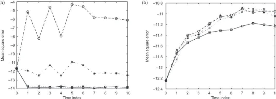
cases, and since the optimal weights are derived using asymptotic arguments, we used as many as 100,000 particles for all algorithms. The result is displayed in Figure 1 (a), and it is clear that operating with true optimal allocation weights improves – as expected – the MSE performance in comparison with the other methods.
The main motivation of Pitt and Shephard [17] for introducing auxiliary parti-cle filtering was to robustify the partiparti-cle approximation to outliers. Thus, we mimic Capp´e et al. [2], Example 7.2.3, and repeat the experiment above for the obser-vation record y0:5 = (−0.652, −0.345, −0.676, 1.142, 0.721, 20), standard devia-tions σv = 1, σ = 0.1, and the smaller particle sample size N = 10,000. Note the large discrepancy of the last observation y5, which in this case is located at a
dis-tance of 20 standard deviations from the mean of the stationary distribution. The outcome is plotted in Figure 1 (b) from which it is evident that the particle filter based on the optimal weights is the most efficient also in this case; moreover, the performance of the standard auxiliary particle filter is improved in comparison with the bootstrap filter. Figure 2 displays a plot of the weight functions t∗4and tP&S4 for the same observation record. It is clear that tP&S
4 is not too far away from the
opti-mal weight function (which is close to symmetric in this extreme situation) in this case, even if the distance between the functions as measured with the supremum norm is still significant.
Finally, we implement the fully adapted filter (with proposal kernels and first-stage weights given by (5.2) and (5.4), respectively) and compare this with the SSAPF based on the same proposal (5.4) and optimal first-stage weights, the latter being given, for x0:k∈ Rk+1and hkdefined in (5.4), by
(5.5) t∗k[πk+1](x0:k) ∝ hk(xk) r
R
R Φ2 k+1[πk+1](xk+1)Rk(xk, dxk+1) = hk(xk) q ˜ σ2 k(xk) + ˜m2k(xk) − 2 ˜mk(xk)φk+1πk+1+ φ2k+1πk+1in this case. We note that hk, that is, the first-stage weight function for the fully adapted filter, enters as a factor in the optimal weight function (5.5). Moreover,
Figure 1. Plot of MSE perfomances (on log-scale) of the bootstrap particle filter (∗), the SSAPF based on optimal weights (¤), and the SSAPF based on the generic weights tP&S
k of Pitt and
Shep-hard [17] (◦). The MSE values are founded on 100,000 particles and 400 runs of each algorithm
Figure 2. Plot of the first-stage importance weight functions t∗
4(unbroken line) and tP&S4 (dashed
line) in the presence of an outlier
recall the definitions (5.3) of ˜mk and ˜σk; in the case of very informative observa-tions, corresponding to σv σ, it holds that ˜σk(x) ≈ σv and ˜mk(x) ≈ yk+1with
good precision for moderate values of x ∈ R (that is, values not too far away from the mean of the stationary distribution of X). Thus, the factor beside hk in (5.5)
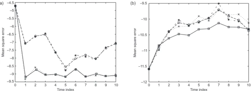
is more or less constant in this case, implying that the fully adapted and optimal first-stage weight filters are close to equivalent. This observation is perfectly con-firmed in Figure 3 (a) which presents MSE performances for σv = 0.1, σ = 1, and
N = 10,000. In the same figure, the bootstrap filter and the standard auxiliary filter
based on generic weights are included for a comparison, and these (particularly the latter) are marred with significantly larger Monte Carlo errors. On the contrary, in the case of non-informative observations, that is, σv σ, we note that ˜σk(x) ≈ σ,
˜
mk(x) ≈ φx and conclude that the optimal kernel is close the prior kernel Q. In
addition, the exponent of hkvanishes, implying uniform first-stage weights for the fully adapted particle filter. Thus, the fully adapted filter will be close to the
boot-strap filter in this case, and Figure 3 (b) seems to confirm this remark. Moreover, the optimal first-stage weight filter does clearly better than the others in terms of MSE performance. –14 –13 –8 –12 –7 –11 –6 –10 –5 –9 –4 Mean square er ror (a) 0 1 2 3 4 5 6 7 8 9 10 Time index –12.4 –12.2 –11.2 –12 –11 –11.8 –10.8 –11.6 –11.4 Mean square er ror (b) 0 1 2 3 4 5 6 7 8 9 10 Time index
Figure 3. Plot of MSE perfomances (on log-scale) of the bootstrap particle filter (∗), the SSAPF based on optimal weights (¤), the SSAPF based on the generic weights tP&S
k (◦), and the fully
adapted SSAPF (×) for the linear/Gaussian model in Section 5.2. The MSE values are computed using 10,000 particles and 400 runs of each algorithm
5.3. ARCH model. Now, let instead
m(Xk) ≡ 0 and σw(Xk) =
q
β0+ β1Xk2.
Here we deal with the classical Gaussian autoregressive conditional heteroscedas-ticity (ARCH) model (see [1]) observed in noise. Since the nonlinear state equa-tion precludes exact computaequa-tion of the filtered means, implementing the optimal first-stage weight SSAPF is considerably more challenging in this case. The prob-lem can however be tackled by means of an introductory zero-stage simulation pass, based on R N particles, in which a crude estimate of φk+1f is obtained.
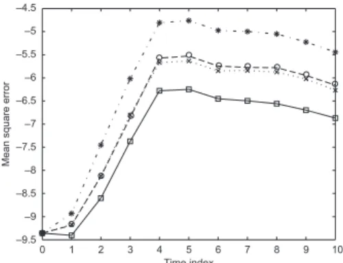
For instance, this can be achieved by applying the standard bootstrap filter with multinomial resampling. Using this approach, we computed again MSE values for the bootstrap filter, the standard SSAPF based on generic weights, the fully adapted SSAPF, and the (approximate) optimal first-stage weight SSAPF, the lat-ter using the optimal proposal kernel. Each algorithm used 10,000 particles and the number of particles in the prefatory pass was set to R = N/10 = 1000, im-plying only a minor additional computational work. An imitation of the true fil-ter means was obtained by running the bootstrap filfil-ter with as many as 500,000 particles. In compliance with the foregoing, we considered the case of informa-tive (Figure 4 (a)) as well as non-informainforma-tive (Figure 4 (b)) observations, cor-responding to (β0, β1, σv) = (9, 5, 1) and (β0, β1, σv) = (0.1, 1, 3), respectively.
Since ˜σk(x) ≈ σv, ˜mk(x) ≈ yk+1in the latter case, we should, in accordance with the previous discussion, again expect the fully adapted filter to be close to that
based on optimal first-stage weights. This is also confirmed in the plot. For the for-mer parameter set, the fully adapted SSAPF exhibits an MSE performance close to that of the bootstrap filter, while the optimal first-stage weight SSAPF is clearly superior.
Figure 4. Plot of MSE perfomances (on log-scale) of the bootstrap particle filter (∗), the SSAPF based on optimal weights (¤), the SSAPF based on the generic weights tP&S
k (◦), and the fully
adapted SSAPF (×) for the ARCH model in Section 5.3. The MSE values are computed using 10,000 particles and 400 runs of each algorithm
5.4. Stochastic volatility. As a final example let us consider the canonical discrete-time stochastic volatility (SV) model [10] given by
Xk+1 = φXk+ σWk+1, Yk = β exp(Xk/2)Vk,
where X = R, and {Wk}∞k=1 and {Vk}∞k=0 are as in Example 5.1. Here X and Y
are log-volatility and log-returns, respectively, where the former are assumed to be stationary. Also this model was treated by Pitt and Shephard [17], who discussed approximate full adaptation of the particle filter by means of a second order Taylor approximation of the concave function x0 7→ log g
k+1(x0). More specifically, by
multiplying the approximate observation density obtained in this way with q(x, x0),
(x, x0) ∈ R2, yielding a Gaussian approximation of the optimal kernel density,
nearly even second-stage weights can be obtained. We proceed in the same spirit, approximating however directly the (log-concave) function x0 7→ g
k+1(x0)q(x, x0)
by means of a second order Taylor expansion of x0 7→ log[g
k+1(x0)q(x, x0)] around
the mode ¯mk(x) (obtained using Newton iterations) of the same:
gk+1(x0)q(x, x0) ≈ rku(x, x0) , gk+1[ ¯mk(x)]q[x, ¯mk(x)] exp ½ − 1 2¯σ2 k(x) [x0− ¯mk(x)]2 ¾ ,
with (we refer to [2], pp. 225–228, for details) ¯σ2
k(x) being the inverted negative
Thus, by letting, for (x, x0) ∈ R2, rk(x, x0) = ruk(x, x0)/
R
Rruk(x, x00)dx00, we obtain (5.6) gk+1(xk+1) dQ(xk, ·) dRk(xk, ·) (xk+1) ≈R
R ruk(xk, x0) dx0 ∝ ¯σk(xk)gk+1[ ¯mk(xk)]q[xk, ¯mk(xk)],and letting, for x0:k∈ Rk+1, tk(x0:k) = ¯σk(xk)gk+1[ ¯mk(xk)]q[xk, ¯mk(xk)] will
imply a nearly fully adapted particle filter. Moreover, by applying the approximate relation (5.6) to the expression (4.1) of the optimal weights, we get (cf. (5.5))
(5.7) t∗k[πk+1](x0:k) ≈
R
R ruk(xk, x0)dx0 rR
R Φ2 k+1[πk+1](x)Rk(xk, dx) ∝ q ¯ σ2 k(xk) + ¯m2k(xk) − 2 ¯mk(xk)φk+1πk+1+ φ2k+1πk+1 × ¯σk(xk)gk+1[ ¯mk(xk)]q[xk, ¯mk(xk)]. In this setting, a numerical experiment was conducted where the two filters above were run, again together with the bootstrap filter and the auxiliary filter based on the generic weights tP&Sk , for parameters (φ, β, σ) = (0.9702, 0.5992, 0.178) (estimated by Pitt and Shephard [18] from daily returns on the U.S. dollar against the U. K. pound stearling from the first day of trading in 1997 and for the next 200 days). To make the filtering problem more challenging, we used a simulated record y0:10of observations arising from the initial state x0= 2.19, being abovethe 2% quantile of the stationary distribution of X, implying a sequence of rel-atively impetuously fluctuating log-returns. The number of particles was set to
N = 5000 for all filters, and the number of particles used in the prefatory filtering
Figure 5. Plot of MSE perfomances (on log-scale) of the bootstrap particle filter (∗), the SSAPF based on optimal weights (¤), the SSAPF based on the generic weights tP&S
k (◦), and the fully
adapted SSAPF (×) for the SV model in Section 5.4. The MSE values are computed using 5000 particles and 400 runs of each algorithm
pass (in which a rough approximation of φk+1πk+1 in (5.7) was computed using
the bootstrap filter) of the SSAPF filter based on optimal first-stage weights was set to R = N/5 = 1000; thus, running the optimal first-stage weight filter is only marginally more demanding than running the fully adapted filter. The outcome is displayed in Figure 5. It is once more obvious that introducing approximate optimal first-stage weights significantly improves the performance also for the SV model, which is recognised as being specially demanding as regards state estimation.
6. APPENDIX — PROOFS
6.1. Proof of Theorem 3.1. Let us recall the updating scheme described in Algorithm 1 and formulate it in the following four isolated steps:
(6.1) {(ξN,i0:k, 1)}Ni=1−−−−−→ {(ξI: Weighting N,i0:k, τkN,i)}Ni=1→
II: Resampling (1st stage)
−−−−−−−−−−−→ {(ˆξN,i0:k, 1)}MN
i=1
III: Mutation
−−−−−→ {(˜ξN,i0:k+1, ˜ωk+1N,i)}MN
i=1 →
IV: Resampling (2nd stage)
−−−−−−−−−−−−→ {(ξN,i0:k+1, 1)}Ni=1,
where we have set ˆξN,i0:k , ξN,IkN,i
0:k , 1 ¬ i ¬ MN. Now, the asymptotic properties
stated in Theorem 3.1 are established by a chain of applications of Theorems 1–4 in [5]. We will proceed by induction: assume that the uniformly weighted particle sample {(ξN,i0:k, 1)}N
i=1is consistent for [L1(Xk+1, φk), φk] and asymptotically
nor-mal for [φk, Ak, L1(Xk+1, φ
k), σk, φk, {
√ N }∞
N =1], with Akbeing a proper set and
σksuch that σk(af ) = |a|σk(f ), f ∈ Ak, a ∈ R. We prove, by analysing each of
the steps I–IV, that this property is preserved through one iteration of the algorithm. I. Define the measure
µk(A) , φkφ(tk1A)
ktk , A ∈ X
⊗(k+1).
Using Theorem 1 of [5] for R(x0:k, ·) = δx0:k(·), L(x0:k, ·) = tk(x0:k) δx0:k(·),
µ = µk, and ν = φk, we conclude that the sample {(ξN,i0:k, τkN,i)}Ni=1is consistent
for [{f ∈ L1(Xk+1, µ
k) : tk|f | ∈ L1(Xk+1, φk)}, µk] = [L1(Xk+1, µk), µk]. Here
the equality is based on the fact that φk(tk|f |) = µk|f | φktk, where the second
fac-tor on the right-hand side is bounded by Assumption (A1). In addition, by applying Theorem 1 of [5] we conclude that {(ξN,i0:k, τkN,i)}N
i=1is asymptotically normal for
(µk, AI,k, WI,k, σI,k, γI,k, {√N }∞
N =1), where
AI,k , {f ∈ L1(Xk+1, µk) : tk|f | ∈ Ak, tkf ∈ L2(Xk+1, φk)}
= {f ∈ L1(Xk+1, µk) : tkf ∈ Ak∩ L2(Xk+1, φk)}, WI,k , {f ∈ L1(Xk+1, µk) : t2k|f | ∈ L1(Xk+1, φk)}
are proper sets, and σ2I,k(f ) , σ2k · tk(f − µkf ) φktk ¸ = σ 2 k[tk(f − µkf )] (φktk)2 , f ∈ AI,k, γI,kf , φk(t2kf ) (φktk)2 , f ∈ WI,k.
II. By Theorems 3 and 4 of [5], {(ˆξN,i0:k, 1)}MN
i=1 is consistent and asymptotically
normal for [L1(Xk+1, µ
k), µk] and [µk, AII,k, L1(Xk+1, µk), σII,k, βµk, {
√ N }∞ N =1], respectively, where AII,k , {f ∈ AI,k : f ∈ L2(Xk+1, µk)} = {f ∈ L2(Xk+1, µk) : tkf ∈ Ak∩ L2(Xk+1, φk)}
is a proper set, and
σII,k2 (f ) , βµk[(f − µkf )2] + σI,k2 (f ) = βµk[(f − µkf )2] +
σ2
k[tk(f − µkf )]
(φktk)2 , f ∈ AII,k.
III. We argue as in step I, but this time for ν = µk, R = Rkp, and L(·, A) =
Rpk(·, wk+11A), A ∈ X⊗(k+2), providing the target distribution
(6.2) µ(A) = µkR p k(wk+11A) µkRpkwk+1 = φkHu k(A) φkHku(Xk+2) = φk+1(A), A ∈ X ⊗(k+2).
This yields, applying Theorems 1 and 2 of [5], that {(˜ξN,ik+1, ˜ωN,ik+1)}MN
i=1 is consistent
for
(6.3) [{f ∈ L1(Xk+2, φk+1), Rpk(·, wk+1|f |) ∈ L1(Xk+1, µk)}, φk+1] = [L1(Xk+2, φk+1), φk+1], where (6.3) follows, since µkRkp(wk+1|f |) φktk = φkHu
k(Xk+2) φk+1|f |, from
(A1), and asymptotically normal for (φk+1, AIII,k+1, WIII,k+1, σIII,k+1, γIII,k+1, {√N }∞ N =1). Here AIII,k+1, {f ∈ L1(Xk+2, φk+1) : Rpk(·, wk+1|f |) ∈ AII,k, Rpk(·, w2k+1f2) ∈ L1(Xk+1, µk)} = {f ∈ L1(Xk+2, φk+1) : Rpk(·, wk+1|f |) ∈ L2(Xk+1, µk), tkRpk(·, wk+1|f |) ∈ Ak∩ L2(Xk+1, φk), Rpk(·, w2k+1f2) ∈ L1(Xk+1, µk)} = {f ∈ L1(Xk+2, φk+1) : Rpk(·, wk+1|f |)Hku(·, |f |) ∈ L1(Xk+1, φk), Hku(·, |f |) ∈ Ak∩ L2(Xk+1, φk), wk+1f2 ∈ L1(Xk+2, φk+1)}
and
WIII,k+1, {f ∈ L1(Xk+2, φk+1) : Rkp(·, w2k+1|f |) ∈ L1(Xk+1, µk)} = {f ∈ L1(Xk+2, φk+1) : wk+1f ∈ L1(Xk+2, φk+1)} are proper sets. In addition, from the identity (6.2) we obtain
µkRkp(wk+1Φk+1[f ]) = 0, where Φk+1is defined in (3.1), yielding, for f ∈ AIII,k+1, σ2III,k+1(f ) , σII,k2 ½ Rpk(·, wk+1Φk+1[f ]) µkRpkwk+1 ¾ +βµkR p k ¡ {wk+1Φk+1[f ] − Rpk(·, wk+1Φk+1[f ])}2 ¢ (µkRpkwk+1)2 = βµk ¡ {Rpk(wk+1Φk+1[f ])}2¢ (µkRpkwk+1)2 +σ 2 k{tkRpk(·, wk+1Φk+1[f ])} (φktk)2(µkRpkwk+1)2 +βµkR p k ¡ {wk+1Φk+1[f ] − Rkp(·, wk+1Φk+1[f ])}2 ¢ (µkRpkwk+1)2 .
Now, applying the equality
{Rpk(·, wk+1Φk+1[f ])}2+ Rkp¡·, {wk+1Φk+1[f ] − Rpk(·, wk+1Φk+1[f ])}2¢ = Rpk(·, w2k+1Φ2k+1[f ]) provides, for f ∈ AIII,k+1, the variance
(6.4) σ2III,k+1(f ) = βφk{tkR
p
k(·, w2k+1Φ2k+1[f ])} φktk+ σk2{Hku(·, Φk+1[f ])}
[φkHku(Xk+2)]2 .
Finally, for f ∈ WIII,k+1,
γIII,k+1f , βµkRpk(w2 k+1f ) (µkRpkwk+1)2 = βφk+1(wk+1f ) φktk φkHu k(Xk+2) .
IV. The consistency for [L1(Xk+2, φ
k+1), φk+1] of the uniformly weighted
particle sample {(ξN,i0:k+1, 1)}N
i=1follows from Theorem 3 in [5]. In addition,
ap-plying Theorem 4 of [5] yields that the same sample is asymptotically normal for [φk+1, AIV,k+1, L1(Xk+2, φk+1), σIV,k+1, φk+1, { √ N }∞ N =1], with AIV,k+1, {f ∈ AIII,k+1: f ∈ L2(Xk+2, φk+1)} = {f ∈ L2(Xk+2, φk+1) : Rpk(·, wk+1|f |)Hku(·, |f |) ∈ L1(Xk+1, φk), Hku(·, |f |) ∈ Ak∩ L2(Xk+1, φk), wk+1f2∈ L1(Xk+2, φk+1)}
being a proper set, and, for f ∈ AIV,k+1,
σ2IV,k+1(f ) , φk+1Φ2k+1[f ] + σ2III,k+1(f ),
with σ2
III,k+1(f ) being defined by (6.4). This concludes the proof of the theorem. 6.2. Proof of Corollary 3.1. We pick f ∈ L2(Xk+2, φk+1) and prove that the
constraints of the set Ak+1 defined in (3.2) are satisfied under Assumption (A3).
Firstly, by Jensen’s inequality,
φk[Rpk(·, wk+1|f |)Hku(·, |f |)] = φk{tk[Rpk(·, wk+1|f |)]2}
¬ φk[tkRpk(·, w2k+1f2)] = φkHku(wk+1f2)
¬ kwk+1kXk+2,∞φkHku(Xk+2) φk+1(f2) < ∞, and, similarly,
φk{[Hku(·, |f |)]2} ¬ kgk+1kX,∞φkHku(Xk+2) φk+1(f2) < ∞.
From this, together with the bound
φk+1(wk+1f2) ¬ kwk+1kXk+2,∞φk+1(f2) < ∞, we conclude that Ak+1= L2(Xk+2, φ
k+1).
To prove L2(Xk+1, φ
k) ⊆ ˜Ak, note that Assumption (A3) implies the equality
˜
Wk= L1(Xk+1, φ
k) and repeat the arguments above.
6.3. Proof of Theorem 3.3. Define, for r ∈ {1, 2} and RN(r) as determined
in Theorem 3.3, the empirical measures
φNk(A) , 1 N N X i=1 δξN,i 0:k, ˜ φNk(A) , RNX(r) i=1 ˜ ωkN,i ˜ ΩN k δ˜ ξN,i0:k(A), A ∈ X ⊗(k+1),
playing the role of approximations of the smoothing distribution φk. Let us define
F0, σ(ξN,i0 ; 1 ¬ i ¬ N ); then the particle history up to the different steps of loop m + 1, m 0, of Algorithm r, r ∈ {1, 2}, is modeled by the filtrations ˆFm ,
Fm∨ σ[ImN,i; 1 ¬ i ¬ RN(r)], ˜Fm+1 , Fm∨ σ[˜ξN,i0:m+1; 1 ¬ i ¬ RN(r)], and
Fm+1, ( ˜ Fm+1∨ σ(Jm+1N,i ; 1 ¬ i ¬ N ) for r = 1, ˜ Fm+1 for r = 2,
respectively. In the coming proof we will describe one iteration of the APF algo-rithm by the following two operations:
{(ξN,i0:k, ωN,ik )}Ni=1 Sampling from ϕNk+1
−−−−−−−−−−−−−−→{(˜ξN,i0:k+1, ˜ωk+1N,i)}Ri=1N(r)→ r = 1: Sampling from ˜φN
0:k+1
where, for A ∈ X⊗(k+2),
ϕNk+1(A) , P(˜ξN,i0:k+10 ∈ A|Fk)
= N X j=1 ωkN,jτkN,j XN `=1ω N,` k τkN,` Rpk(ξN,j0:k, A) = φ N k[tkRpk(·, A)] φN ktk (6.5)
for some index i0 ∈ {1, . . . , RN(r)} (given Fk, the particles ˜ξN,i0:k+1, 1 ¬ i ¬ RN(r), are i.i.d.). Here the initial weights {ωN,ik }Ni=1are all equal to one for r = 1.
The second operation is valid since, for any i0 ∈ {1, . . . , N },
P(ξN,i0 0:k+1 ∈ A| ˜Fk+1) = RNX(r) j=1 ˜ ωk+1N,j ˜ ΩN k+1 δ˜ ξN,j0:k+1(A) = ˜φ N 0:k+1(A), A ∈ X⊗(k+2).
The fact that the evolution of the particles can be described by two Monte Carlo operations involving conditionally i.i.d. variables makes it possible to analyse the error using the Marcinkiewicz–Zygmund inequality (see [16], p. 62).
Using this, set, for 1 ¬ k ¬ n, (6.6) αNk(A) ,
R
A dαNk dϕN k (x0:k)ϕNk(dx0:k), A ∈ X⊗(k+1), with, for x0:k ∈ Xk+1, dαNk dϕN k (x0:k) , wk(x0:k)Hu k. . . Hn−1u (x0:k, Xn+1) φNk−1tk−1 φN k−1Hk−1u . . . Hn−1u (Xn+1) .Here we apply the standard convention Hu
` . . . Hmu , Id if m < `. For k = 0 we define α0(A) ,
R
A dα0 dς (x0)ς(dx0), A ∈ X , with, for x0 ∈ X, dα0 dς (x0) , w0(x0)H0u. . . Hn−1u (x0, Xn+1) ν[g0H0u. . . Hn−1u (·, Xn+1)] .Similarly, put, for 0 ¬ k ¬ n − 1, (6.7) βkN(A) ,
R
A dβN k d ˜φN k (x0:k) ˜φNk(dx0:k), A ∈ X⊗(k+1), where, for x0:k∈ Xk+1, dβN k d ˜φN k (x0:k) , Hu k. . . Hn−1u (x0:k, Xn+1) ˜ φN kHku. . . Hn−1u (Xn+1) .The following powerful decomposition is an adaption of a similar one derived by Olsson et al. [14], Lemma 7.2 (the standard SISR case), being in turn a refine-ment of a decomposition originally presented by Del Moral [4].
LEMMA6.1. Let n 0. Then, for all f ∈ Bb(Xn+1), N 1, and r ∈ {1, 2},
(6.8) φ˜N0:nf − φnf = n X k=1 ANk(f ) +1{r = 1}n−1X k=0 BNk(f ) + CN(f ), where ANk(f ) , XRN(r) i=1 (dαNk/dϕNk)(˜ξ N,i 0:k)Ψk:n[f ](˜ξN,i0:k) XRN(r) j=1 (dαNk/dϕNk)(˜ξ N,j 0:k) − αNkΨk:n[f ], BkN(f ) , XN
i=1(dβkN/d ˜φNk)(ξN,i0:k)Ψk:n[f ](ξN,i0:k)
XN j=1(dβkN/d ˜φNk)(ξ N,j 0:k) − βkNΨk:n[f ], CN(f ) , XN i=1(dβ0|n/dς)(ξ N,i 0 )Ψ0:n[f ](ξN,i0 ) XN j=1(dβ0/dς)(ξ N,i 0 ) − φnΨ0:n[f ],
and the operators Ψk:n: Bb(Xn+1) → B
b(Xn+1), 0 ¬ k ¬ n, are, for some fixed points ˆx0:k∈ Xk+1, defined by Ψk:n[f ] : x0:k7→ H u k. . . Hn−1u f (x0:k) Hu k. . . Hn−1u (x0:k, Xn+1) − H u k. . . Hn−1u f (ˆx0:k) Hu k. . . Hn−1u (ˆx0:k, Xn+1) .
P r o o f. Consider the decomposition
˜ φN0:nf − φnf = Xn k=1 " ˜ φN kHku. . . Hn−1u f ˜ φN kHku. . . Hn−1u (Xn+1) − φ N k−1Hk−1u . . . Hn−1u f φN k−1Hk−1u . . . Hn−1u (Xn+1) # +1{r = 1}n−1X k=0 " φN kHku. . . Hn−1u f φN kHku. . . Hn−1u (Xn+1) − φ˜ N kHku. . . Hn−1u f ˜ φN kHku. . . Hn−1u (Xn+1) # + φ˜ N 0 H0u. . . Hn−1u f ˜ φN 0 H0u. . . Hn−1u (Xn+1) − φnf.
We will show that the three parts of this decomposition are identical with the three parts of (6.8). For k 1, using the definitions (6.5) and (6.6) of ϕN
respectively, and following the lines of Olsson et al. [14], Lemma 7.2, we obtain φNk−1Hk−1u . . . Hn−1u Hn−1u f φN k−1Hk−1u . . . Hn−1u (Xn+1) = ϕNk · wk(·)Hku. . . Hn−1u f (·)(φNk−1tk−1) φN k−1Hk−1u . . . Hn−1u (Xn+1) ¸ = αNk · Ψk:n[f ](·) + Hu k. . . Hn−1u f (ˆx0:k) Hu k. . . Hn−1u (ˆx0:k, Xn+1) ¸ = αNkΨk:n[f ] + H u k. . . Hn−1u f (ˆx0:k) Hu k. . . Hn−1u (ˆx0:k, Xn+1) .
Moreover, by definition, we get ˜ φN kHku. . . Hn−1u f ˜ φN kHku. . . Hn−1u (Xn+1) = XRN(r) i=1 (dαNk /dϕNk)(˜ξ N,i 0:k)Ψk:n[f ](˜ξN,i0:k) XRN(r) j=1 (dαNk/dϕNk)(˜ξ N,j 0:k) + H u k. . . Hn−1u f (ˆx0:k) Hu k. . . Hn−1u (ˆx0:k, Xn+1), which yields ˜ φN kHku. . . Hn−1u f ˜ φN k Hku. . . Hn−1u (Xn+1) − φ N k−1Hk−1u . . . Hn−1u f φN k−1Hk−1u . . . Hn−1u (Xn+1) ≡ ANk(f ).
Similarly, for r = 1, using the definition (6.7) of βN k, ˜ φN 0:kHk−1u . . . Hn−1u f ˜ φN 0:kHk−1u . . . Hn−1u (Xn+1) = βNk · Hku. . . Hn−1u f (·) Hu k. . . Hn−1u (Xn+1) ¸ = βNk · Ψk:n[f ](·) + Hu k. . . Hn−1u f (ˆx0:k) Hu k. . . Hn−1u (ˆx0:k, Xn+1) ¸ = βNk Ψk:n[f ] + H u k. . . Hn−1u f (ˆx0:k) Hu k. . . Hn−1u (ˆx0:k, Xn+1) ,
and applying the obvious relation
φNkHku. . . Hn−1u f φN
kHku. . . Hn−1u (Xn+1)
= XN
i=1(dβNk/d ˜φNk)(ξN,i0:k)Ψk:n[f ](ξN,i0:k)
XN j=1(dβkN/d ˜φNk)(ξN,j0:k) + H u k. . . Hn−1u f (ˆx0:k) Hu k. . . Hn−1u (ˆx0:k, Xn+1),
we obtain the identity
φN kHku. . . Hn−1u f φN kHku. . . Hn−1u (Xn+1) − φ˜ N kHku. . . Hn−1u f ˜ φN kHku. . . Hn−1u (Xn+1) ≡ BNk (f ).
![Figure 1. Plot of MSE perfomances (on log-scale) of the bootstrap particle filter (∗), the SSAPF based on optimal weights (¤), and the SSAPF based on the generic weights t P&S k of Pitt and Shep-hard [17] (◦)](https://thumb-eu.123doks.com/thumbv2/123doknet/12278994.322296/16.892.167.709.177.412/figure-perfomances-bootstrap-particle-optimal-weights-generic-weights.webp)