Série Scientifique
Scientific Series
2002s-07A Structural Analysis of the
Correlated Random Coefficient
Wage Regression Model
Christian Belzil, Jörgen Hansen
CIRANO
Le CIRANO est un organisme sans but lucratif constitué en vertu de la Loi des compagnies du Québec. Le financement de son infrastructure et de ses activités de recherche provient des cotisations de ses organisations-membres, d’une subvention d’infrastructure du ministère de la Recherche, de la Science et de la Technologie, de même que des subventions et mandats obtenus par ses équipes de recherche.
CIRANO is a private non-profit organization incorporated under the Québec Companies Act. Its infrastructure and research activities are funded through fees paid by member organizations, an infrastructure grant from the Ministère de la Recherche, de la Science et de la Technologie, and grants and research mandates obtained by its research teams.
Les organisations-partenaires / The Partner Organizations
•École des Hautes Études Commerciales •École Polytechnique de Montréal •Université Concordia
•Université de Montréal
•Université du Québec à Montréal •Université Laval
•Université McGill
•Ministère des Finances du Québec •MRST
•Alcan inc. •AXA Canada •Banque du Canada
•Banque Laurentienne du Canada •Banque Nationale du Canada •Banque Royale du Canada •Bell Canada
•Bombardier •Bourse de Montréal
•Développement des ressources humaines Canada (DRHC) •Fédération des caisses Desjardins du Québec
•Hydro-Québec •Industrie Canada
•Pratt & Whitney Canada Inc. •Raymond Chabot Grant Thornton •Ville de Montréal
© 2002 Christian Belzil et Jörgen Hansen. Tous droits réservés. All rights reserved. Reproduction partielle permise
avec citation du document source, incluant la notice ©.
Short sections may be quoted without explicit permission, if full credit, including © notice, is given to the source.
Ce document est publié dans l’intention de rendre accessibles les résultats préliminaires de la recherche effectuée au CIRANO, afin de susciter des échanges et des suggestions. Les idées et les opinions émises sont sous l’unique responsabilité des auteurs, et ne représentent pas nécessairement les positions du CIRANO ou de ses partenaires.
This paper presents preliminary research carried out at CIRANO and aims at encouraging discussion and comment. The observations and viewpoints expressed are the sole responsibility of the authors. They do not necessarily represent positions of CIRANO or its partners.
A Structural Analysis of the Correlated Random Coefficient
Wage Regression Model
*Christian Belzil
†and Jörgen Hansen
‡We estimate a finite mixture dynamic programming model of schooling decisions in which the log wage regression function is set in a random coefficient framework. The model allows for absolute and comparative advantages in the labor market and assumes that the population is composed of 8 unknown types. Overall, labor market skills (as opposed to taste for schooling) appear to be the prime factor explaining schooling attainments. The estimates indicate a higher cross-sectional variance in the returns to experience than in the returns to schooling. From various simulations, we find that the sub-population mostly affected by a counterfactual change in the utility of attending school is composed of individuals who have any combination of some of the following attributes; absolute advantages in the labor market, high returns to experience, low utility of attending school and relatively low returns to schooling. Unlike what is often postulated in the average treatment effect literature, the weak correlation (unconditional) between the returns to schooling and the individual reactions to treatment is not sufficient to reconcile the discrepancy between OLS and IV estimates of the returns to schooling often found in the literature.
Nous estimons un modèle de programmation dynamique des choix en éducation dans lequel la fonction de régression logarithmique du salaire dépend de coefficients aléatoires. Ce modèle permet de tenir compte des avantages absolus et comparés des individus sur le marché de l’emploi et part du principe que la population est composée de huit types inconnus. Dans l’ensemble, les qualifications sur le marché du travail (par opposition au goût de s’instruire) semblent être le principal facteur permettant d’expliquer les niveaux de scolarité. Nos estimations indiquent une plus forte variance transversale dans les rendements de l’éducation. À partir de plusieurs simulations, nous trouvons que la sous-population qui se trouve le plus affecté par un changement contrefactuel dans le niveau d’utilité de la fréquentation scolaire est celle composée d’individus possédant une combinaison des attributs suivants : avantage absolu sur le marché du travail, rendements élevés de l’expérience, faible niveau d’utilité par rapport à la fréquentation scolaire et rendements de l’éducation relativement bas. Contrairement à ce qui est souvent postulé dans la littérature, la corrélation faible (non conditionnelle) entre les rendements de l’éducation et les réactions individuelles aux traitements n’est pas une condition suffisante pour réconcilier les différences que l’on retrouve souvent dans la littérature entre les résultats des estimations par MCO et par VI des rendements de l’éducation.
Mots clés : Coefficients aléatoires, Rendements de l’éducation, Avantages comparés, Programmation
dynamique, Auto-sélection dynamique
Keywords : Random Coefficient, Returns to Schooling, Comparative Advantages, Dynamic
Programming, Dynamic Self-Selection
JEL Classification : J2-J3
1
Introduction and Objectives
In this paper, we investigate the empirical properties of the correlated random co-e±cient wage regression model (CRCWRM) using a structural dynamic program-ming model.1 The term \correlated random coe±cient wage regression model"
refers to the standard Mincerian log wage regression function in which the coef-¯cients may be arbitrarily correlated with the regressors (education and experi-ence). While the comparative advantages representation of the labor market is far from being new (Roy, 1951, Becker and Chiswick, 1966 and Willis and Rosen, 1979), economists have only recently paid particular attention to the speci¯cation and the estimation of linear wage regression models set in a random coe±cient framework (Heckman and Vitlacyl (1998, 2000), Wooldridge (1997, 2000), Angrist and Imbens (1994), Card (2000) and Meghir and Palme (2001)). In this branch of the literature, it is customary to estimate the log wage regression function using Instrumental Variable (IV) techniques and interpret the estimates in a framework where the returns to schooling are individual speci¯c. This surge of new research is understandable. In a context where schooling is understood as the outcome of individual decision making within a dynamic framework, rational individuals base their schooling decisions partly on absolute and comparative advantages in the labor market and partly on their taste for schooling. As a consequence, the random coe±cients (the returns to schooling and experience), as opposed to only the individual speci¯c intercept terms, will normally be correlated with individual schooling attainments.
Estimating the returns to schooling within a random coe±cient framework is di±cult. In general, the use of IV techniques requires linear separability between the instruments and the error term in the treatment (schooling) equation. Very often, estimates of the return to schooling are only obtained for a sub-population (i.e. the e®ect of treatment on the treated) and those who use standard IV techniques are faced with the consequences of using \weak instruments" (see Staiger and Stock, 1997).
In a linear wage regression, individual di®erences in the intercept term rep-resent a measure of absolute advantage in the labor market while di®erences in slopes re°ect individual comparative advantages in human capital acquisition via schooling and experience. While it might be tempting to focus solely on heterogeneity in the returns to schooling (and assume homogeneous returns to experience), this approach is likely to be unsatisfactory. If the returns to school-ing and experience are truly correlated, ignorschool-ing individual di®erences in the return to labor market experience is likely to a®ect the estimates of the returns to schooling as well as the causal link between labor market ability and school-ing (dynamic self-selection). Modelschool-ing wage regressions in a random coe±cient
1The term \correlated random coe±cient wage regression model" is also used in Heckman
framework therefore requires the allowance for heterogeneity in the returns to experience.2 As it stands, very little is known about the empirical properties of
the CRCWRM. Those interested in estimating the returns to schooling by IV techniques usually ignore higher moments such as the variance of the returns to schooling and experience, or use a reduced-form framework which cannot disclose the covariances between realized schooling and the individual speci¯c coe±cients. However, these quantities are important. They may shed light on the importance of comparative advantages in the labor market and help comprehend the deter-minants of individual schooling attainments. Finally, they may help quantify the \Ability Bias" (OLS bias) arising in estimating the returns to schooling using regression techniques.
Despite the recent interest in the random coe±cient speci¯cation shown by labor economists and applied econometricians, there is no obvious reason to be-lieve that the CRCWRM is superior to other potential speci¯cations of the wage regression function. The comparative advantages representation of the wage re-gression function is one possible way to introduce heterogeneity in the returns to schooling. It is well known that heterogeneity in the realized returns to schooling may also arise if the local returns change with the level of schooling. In a recent paper, Belzil and Hansen (2001a) used a structural dynamic programming model to obtain °exible estimates of the wage regression function from the National Longitudinal Survey of Youth (NLSY). They found that the log wage regression is highly convex and found returns to schooling much lower than what is usually reported in the existing literature although the local returns may °uctuate be-tween 1% (or less) and 13% per year.3 However, as the model estimated in Belzil
and Hansen (2001a) is set in a classical framework where market skill heterogene-ity is captured solely in the intercept term of the wage regression, it is di±cult to say if the high degree of convexity is explained by a composition e®ect (i.e.; the local returns at high levels of schooling are estimated from a sub-population which has higher returns to schooling than average) and if the low returns re-ported are explained by an absence of control for heterogeneity in the returns to schooling (and experience).
While both hypotheses (skill heterogeneity and non-linearities) are not mu-tually exclusive, they are di±cult to confront simultaneously because in most panel data sets, individual wages are observed for a given level of schooling. The non-linearity speci¯cation and the skill heterogeneity (random coe±cient) spec-i¯cation should be regarded as non-nested models. Nevertheless, a random
co-2Individual di®erences in the return to experience may be explained by comparative
advan-tages in on-the-job training, learning on the job, job search or any other type of post-schooling activities enhancing market wages. Allowing for heterogeneity in the returns to experience is especially important if individual post-schooling human capital investments are unobserved (which is the case in most data sets).
3The model also implies a positive correlation between market ability and realized schooling
e±cient regression model provides a realistic framework to evaluate the relative importance of labor markets skills and taste for schooling in explaining cross-sectional di®erences in schooling attainments, and to illustrate the importance of comparative advantages. For this reason, it deserves some attention.
Our main objective is to investigate the empirical properties of the CRCWRM. These include the population average returns to schooling and experience, the relative dispersions in the returns to schooling and experience, and the relative importance of labor market skills and individual speci¯c taste for schooling in explaining cross-sectional di®erences in schooling attainments. We estimate a ¯-nite mixture structural dynamic programming model of schooling decisions with 8 unknown types of individuals, where each type is characterized by a speci¯c log wage regression function (linear) as well as a speci¯c utility of attending school. The estimation of a mixed likelihood function has two main advantages. It can capture any arbitrary correlation between any of the heterogeneity components and it obviates the need to incorporate all parents' background variables in each single heterogeneity component or to select, somewhat arbitrarily, which het-erogeneity components are correlated with household background variables and which ones are not.
A second objective is to illustrate the importance of population heterogene-ity and, more speci¯cally, to analyze the characteristics of the sub-population (s) most a®ected by an exogenous change in the utility of attending school. This is an important issue. In the literature, estimates of the returns to schooling obtained using instrumental variable techniques are often higher than OLS estimates.4 It
is often postulated that these results are explained by the fact that those indi-viduals more likely to react to an exogenous increase in the utility of attending school must have higher returns to schooling than average. As far as we know, this claim has neither been proved nor veri¯ed empirically in any direct fashion. To do so, we investigate how individual speci¯c reactions to a generous coun-terfactual college attendance subsidy are correlated with individual absolute and comparative advantages.
A third and ¯nal objective is to investigate the notion of \Ability Bias" in a context where the notion is much deeper than the usual correlation between the individual speci¯c intercept terms of the wage regression and realized schooling attainments. As market ability heterogeneity is multi-dimensional in our model, our estimate of the Ability Bias (OLS bias) is not only explained by the corre-lation between the individual speci¯c intercept term and realized schooling but also by the simultaneous correlations between schooling and experience and the individual speci¯c deviations from population average returns to schooling and experience.
4At the same time, empirical evidence also suggests that standard wage regressions
aug-mented with observable measures of ability (such as test scores and the like) lead to a decrease in the estimated returns to schooling.
The model is implemented on a panel of white males taken from the National Longitudinal Survey of Youth (NLSY). The panel covers a period going from 1979 until 1990. The main results are as follows. Consistent with the results reported in Belzil and Hansen (2001a), we ¯nd population average returns to schooling which are much below those reported in the existing literature. Our estimates are also much lower than those obtained using standard OLS techniques. The average return to experience upon entering the labor market (0.0863) exceeds the average return to schooling (0.0576) and we ¯nd more cross-sectional variability in the returns to experience than in the returns to schooling. The returns to schooling and experience are found to be positively correlated. Not surprisingly, the correlated random coe±cient wage regression model ¯ts wage data very well. It can explain as much as 78.5% of the variation in realized wages. Overall, the dynamic programming model indicates that labor market skills are the prime fac-tor explaining schooling attainments as 82% of the explained variation is indeed explained by individual comparative and absolute advantages in the labor market and only 18% is explained by individual di®erences in taste for schooling. More-over, realized schooling attainments are more strongly correlated with individual di®erences in returns to experience than in returns to schooling.
The importance of individual speci¯c returns to experience is well illustrated by the di®erent reactions to a common post-high school education subsidy. In particular, those types more likely to obtain a high level of schooling appear par-ticularly una®ected by this subsidy. This illustrates the fundamental weakness of various estimation methods based on \exogenous instruments". As only a sub-set of the population is a®ected by this exogenous policy change, standard IV estimates would be based on individuals who have a low propensity to acquire schooling. It is therefore di±cult to conduct reliable inference about the popu-lation returns to schooling. We ¯nd that the sub-popupopu-lation mostly a®ected is composed of individuals who have any combination of some of the following at-tributes; absolute advantages in the labor market, high returns to experience, low utility of attending school and, relatively low returns to schooling. Unlike what is often postulated in the average treatment e®ect literature, the weak correlation (unconditional) between the returns to schooling and the individual reactions to treatment is not su±cient to reconcile the discrepancy between OLS and IV estimates of the returns to schooling often found in the literature.
The paper is structured as follows. The empirical dynamic programming model is exposed in Section 2. The goodness of ¯t is evaluated in Section 3. A discussion of the estimates of the return to schooling and experience are found in Section 4. In Section 5, we illustrate the links between labor market skills and dynamic self-selection. In Section 6, we analyze the determinants of the individ-ual speci¯c reactions to a college attendance subsidy and examine a proposition often claimed in the \Average Treatment E®ects" literature; that the discrepancy between OLS and IV estimates of the returns to schooling may be explained by the relatively higher returns experienced by those a®ected by exogenous policy
changes. In Section 7, we discuss the links between our estimates and those reported in the literature and re-examine the notion of Ability Bias in a con-text where the regression function allows for a rich speci¯cation of absolute and comparative advantages. The conclusion is in Section 8.
2
An Empirical Dynamic Programming Model
of Schooling Decisions with Comparative
Ad-vantages
In this section, we introduce the empirical dynamic programming model. While the theoretical structure of the problem solved by a speci¯c agent is similar to the model found in Belzil and Hansen (2001a), the di®erent stochastic speci¯cation and, especially, the allowance for a rich speci¯cation of absolute and comparative advantages requires a full presentation.
Young individuals decide sequentially whether it is optimal or not to enter the labor market or continue accumulate human capital. Individuals maximize discounted expected lifetime utility over a ¯nite horizon T and have identical preferences. Both the instantaneous utility of being in school and the utility of work are logarithmic. The control variable, dit; summarizes the stopping rule.
When dit = 1; an individual invests in an additional year of schooling at the
beginning of period t. When dit = 0, an individual leaves school at the beginning
of period t (to enter the labor market). Every decision is made at the beginning the period and the amount of schooling acquired by the beginning of date t is denoted Sit:
2.1
The Utility of Attending School
The instantaneous utility of attending school, Us(:); is formulated as the following
equation5
Us(:) = Ã(Sit) + À»i + " »
it (1)
in which "»it » i:i:d N(0; ¾»2) represents a stochastic utility shock, the term À » i
rep-resents individual heterogeneity (ability) a®ecting the utility of attending school and Ã(:) captures the co-movement between the utility of attending school and grade level.
We assume that individuals interrupt schooling with exogenous probability ³ and, as a consequence, the possibility to take a decision depends on a state
5The utiliy of school could be interpreted as the monetary equivalent (on a per hour basis)
variable Iit:6 When Iit = 1; the decision problem is frozen for one period. If
Iit = 0; the decision can be made. When an interruption occurs, the stock of
human capital remains constant over the period.7
2.2
The Utility of Work
Once the individual has entered the labor market, he receives monetary income ~
wt; which is the product of the yearly employment rate, et; and the wage rate,
wt: The instantaneous utility of work, Uw(:)
Uw(:) = log( ~wt) = log(et¢ wt)
2.3
The Correlated Random Coe±cient Wage Regression
Model
The log wage received by individual i, at time t, is given by
log wit = '1i¢ Sit+ ¸i¢ ('2¢ Experit+ '3¢ Exper2it) + Àiw+ "wit (2)
where '1i is the individual speci¯c wage return to schooling and ¸i is an
indi-vidual speci¯c factor multiplying the e®ect of experience ('2) and the e®ect of experience squared ('3). The term Àw
i represents an individual speci¯c intercept
term. We assume that
'1i = ¹'1+ !1i
¸i = ¹¸ + !2i
where ¹'1 and ¹¸ represent population averages. Following the convention used in the literature, it is convenient to specify the wage regression as a heteroskedastic regression function
log wit= ¹'1¢ Sit+ ¹'¤2:¢ Experit+ ¹'¤3:¢ Exper2it+ »it (3)
where
¹
'¤2 = ¹¸¢ '2
6The interruption state is meant to capture events such as illness, injury, travel, temporary
work, incarceration or academic failure.
7The NLSY does not contain data on parental transfers and, in particular, does not allow
a distinction in income received according to the interruption status. As a consequence, we ignore the distinction between income support while in school and income support when school is interrupted. In the NLSY, we ¯nd that more than 85% of the sample has never experienced school interruption.
¹
'¤3 = ¹¸¢ '3
»it = Àwi + !1i¢ Sit+ !2i¢ ('2¢ Experit+ '3:¢ Exper2it) + "wit
Estimating the population average returns to schooling and experience ( ¹'1,
¹ '¤
2 and ¹'¤3 ) is rendered di±cult by the fact that typically
Corr( »it; Sit)6= 0
Corr( »it; Experit)6= 0
and also by the fact that Ài» and Sit cannot be separated linearly.8
2.4
The Employment Rate
The employment rate, eit; is also allowed to depend on accumulated human capital
(Sit and Experit) so that
ln e¤it= ln 1 eit
= Àie+ ·1¢ Sit+ ·2 ¢ Experit + ·3¢ Exper2it+ "eit (4)
where Àie is an individual speci¯c intercept term, ·1 represents the employment
security return to schooling, both ·2 and ·3 represent the employment security
return to experience.9 The random shock "e
itis normally distributed with mean 0
and variance ¾2
e: All random shocks (" »
it; "wit; "eit) are assumed to be independent.
2.5
The Value Functions
We only model the decision to acquire schooling beyond 6 years (as virtually every individual in the sample has completed at least six years of schooling). We set T to 65 years and the maximum number of years of schooling to 22. Dropping the individual subscript, the value function associated with the decision to remain in school, given accumulated schooling St , denoted Vts(St; ´t); can be expressed as
Vts(St; ´t) = ln(»t) + ¯f³ ¢ EVt+1I (St+1; ´t+1) (5)
+(1¡ ³) ¢ EMax[Vs
t+1(St+1; ´t+1); Vt+1w (St+1; ´t+1)]g
8See Heckman and Vytlacil (1998), Rosenzweig and Wolpin (2000) and Belzil and Hansen
(2001a) for a discussion of these correlations.
9It follows that the expected value and the variance of the employment rate are given by
where VI
t+1(St+1; ´t+1) denotes the value of interrupting schooling acquisition.
Since we cannot distinguish between income support while in school and income support when school is interrupted, the value of interrupting schooling acquisition is identical to the value of attending school. VI
t+1(St+1; ´t+1); can be expressed
as follows.
Vt+1I (St+1; ´t+1) = log(»t+1) + ¯f³ ¢ EVt+2I (St+2; ´t+2)
+(1¡ ³) ¢ EMax[Vs
t+2(St+2; ´t+2); Vt+2w (St+2; ´t+2)]g (6)
The value of stopping school (that is entering the labor market), Vw
t (St; ´t), is
given by
Vtw(St; ´t) = ln(wit¢ eit) + ¯E(Vt+1j dt= 0) (7)
where E(Vt+1j dt= 0) is simply
E(Vt+1j dt = 0) = T X j=t+1 ¯j¡(t+1)(¡ exp(¹j+ 1 2¾ 2 e)+'1(Sj)+¸¢['2:Experj+'3:Experj2])
is simply the expected utility of working from t + 1 until T . Using the termi-nal value and the distributiotermi-nal assumptions about the stochastic shocks, the probability of choosing a particular sequence of discrete choices can readily be expressed in closed form.
2.6
Unobserved Ability in School and in the Labor
Mar-ket
We assume that there are K types of individuals. Each type (k) is endowed with a vector (À»k; Àw
k; Àek; '1k; ¸k) for k = 1; 2:::K . The results reported in this paper
are for the case K = 8. The probability of belonging to type k; pk; is estimated
using logistic transform
pk =
exp(qk)
P8
j=1exp(qj)
and with the restriction that q8 = 0.10
10As discussed in Belzil and Hansen (2001a), identi¯cation of most parameters is relatively
straightforward. However, in order to reduce the degree of identi¯cation, we ¯xed the discount rate to 3% per year (an estimate practically identical to the estimate found in Belzil and Hansen (2001a). The degree of under-identi¯cation arising in estimating structural dynamic programming models is discussed in details in Rust (1994) and Magnac and Thesmar (2001).
2.7
The Likelihood Function
Constructing the likelihood function (for a given type k) is relatively straightfor-ward. It has three components; the probability of having spent at most ¿ years in school (L1k), the probability of entering the labor market in year ¿ + 1; at
observed wage w¿ +1 (denoted L2k) and the density of observed wages and
em-ployment rates from ¿ + 2 until 1990 (denoted L3k): L1k can easily be evaluated
using (5) and (6), while L2kcan be factored as the product of a normal conditional
probability times the marginal wage density. Finally L3k is just the product of
wage densities and employment densities. For a given type k, the likelihood is therefore Lk = L1k¢ L2k¢ L3k and the log likelihood function to be maximized is
log L = log
8
X
k=1
pk¢ Lk (8)
where each pk represents the population proportion of type k.
3
Accuracy of Predicted Schooling and Predicted
Wages
Evidence presented in Table 1A shows clearly that the model is capable of ¯tting the data quite well. A comparison between actual and predicted frequencies reveals that, except for the very low levels of schooling, our model predicts a pattern which is practically identical to the one found in the data. In particular, we are able to predict the large frequencies at 12 years and 16 years. The ¯t is comparable to what is found in Belzil and Hansen (2001a and 2001b), in which data on household background (parents' education and income, number of siblings and the like) are used explicitly in the utility of attending school as well as in the wage regression.
Using the structural estimates, it is easy to compute a type speci¯c expected schooling attainments. These are reported in Table 1B. The type speci¯c attain-ments range from 9.4 years (type 4) to 13.7 years (type 3). An in-depth analysis of the links between schooling and individual speci¯c absolute and comparative advantages is delayed to Section 5.
It is also straightforward to use the simulated values of schooling and experi-ence to simulate series of realized lifetime wages. These series can be used to infer the fraction of the variance of realized wages which is explained by the individual speci¯c regression functions. To investigate the goodness of ¯t, we have simu-lated wages for a cohort of individuals aged 30 in 199011. The results reported in
Table 1C indicate that random coe±cient model explains 78.9% of the observed (realized) variation in wages. This is much larger than what is usually reported
in the literature, in which standard OLS regressions of wages on schooling and experience typically result in values of R2 ranging between 0.20 and 0.25 (see
Card, 2000).
4
Absolute and Comparative Advantages in the
Labor Market: Some Estimates
In this section, we discuss of the estimates of the return to schooling and expe-rience. Note that he estimation of a ¯nite mixture dynamic programming model not only allows us to estimate the population average returns to schooling and experience but also the cross-sectional variability in the returns. This is a novel feature. As far as we know, no one has ever been able to obtain estimates of the variances of the returns to schooling and experience.12
The individual speci¯c estimates of the wage regression function (the returns to schooling and experience as well as the individual speci¯c intercept terms measuring absolute advantages in the labor market) are found in Table 2A. Our estimates of the returns to schooling range from 0.0265 (type 7) to 0.0879 (type 2) while our estimates of the individual speci¯c ¸0s (ranging from 0.1453 to 1.0866)
imply that the returns to experience upon entrance in the labor market range from 0.0197 (type 6) to 0.1477 (type 5). Given the estimates for '2 (0.1359) and
'3 (-0.0040), the ordering based on the ¸0s is identical to the ordering based on
the product of ¸ and '2 for the most part of the life cycle and, especially, for the early post-schooling period. As an illustration, the individual speci¯c returns to experience measured after 8 years of experience (a level higher than the average level of experience measured in 1990) are 0.0719 (type 1), 0.0222 (type 2), 0.0141 (type 3), 0.0191 (type 4), 0.0781 (type 5), 0.0105 (type 6), 0.0690 (type 7) and 0.0246 (type 8).
Overall, and as reported in Belzil and Hansen (2001a), our estimates of the re-turn to schooling are much lower than those reported in the existing literature.13
The population average return to schooling (0.0575) is smaller than the popu-lation average return to experience upon entrance in the labor market (0.0863). Interestingly, the high degree of dispersion in ¸ implies a higher standard de-viation in the returns to experience (0.0527) than in the returns to education (0.0218). Upon reviewing the estimated ¸0s and the '01s; it is also noticeable, al-though not surprising, that the returns to schooling and experience are positively correlated. The correlation between '1i and ¸i is around 0.11 and is discussed in
12Very often, those who focus on the return to schooling use a proxy variable for experience.
Rosenzweig and Wolpin (2000) present a critical analysis of empirical work devoted to the estimation of the returns to schooling, which ignores post-schooling human capital investment.
13However, in Belzil and Hansen (2001a), the wage regression function is estimated °exibly
using spline techniques. There are 8 di®erent local returns which range 0.4% per year to 12.0% per year.
more details below (Section 6). It may be explained by the fact that labor market skills which enhance wage growth (job training, job search, etc..) are positively correlated with academic skills which are rewarded in the labor market. This result has clear impact for the nature of dynamic self-selection. Those endowed with high returns to education will not necessarily obtain a high level of schooling because they will be facing a higher opportunity cost of attending school.
While it is di±cult to evaluate the relative degree of heterogeneity in taste for schooling and in the returns to human capital without performing simulations, it is nevertheless informative to examine the estimates of the intercept terms of the utility of attending school (reported in Table 2B). Clearly, individual di®erences in the intercept terms of the taste for schooling appear as important as di®erences in the intercept terms of the wage equation. The intercept terms for the utility of attending school range from -1.7791 (type 2) to -0.6397 (type 7). Interestingly, even after allowing for 8 types, the high degree of variability (as well as the signi¯cance level) of the spline estimates shows that the utility of attending school undoubtedly varies with school level.
Table 3 summarizes the type speci¯c rankings according to all heterogeneity dimensions as well as the level of expected schooling. In an empirical model char-acterized by a rich speci¯cation for skill heterogeneity, the self-selection process is intricate. Individuals take optimal schooling decisions based on their individ-ual speci¯c taste for schooling and their absolute and comparative advantages in the labor market. While some individuals are endowed with a high taste for schooling (as can be seen from Table 2B), schooling decisions are largely a®ected by the combination of comparative advantages (returns to schooling and expe-rience) and absolute advantages (intercept terms of the wage regression). As a consequence, it will be impossible to associate a de¯nite set of attributes (say, high or low return to human capital) to each speci¯c type on the basis of their sole expected schooling attainments. Nevertheless, our model is su±ciently rich to capture di®erences in comparative advantages among types of individuals that might obtain similar levels of schooling.
To illustrate this, consider the set of individuals (type 1, type 2, type 4 and type 7) who are predicted to obtain a relatively lower level of schooling than the rest of the population. Type 7 individuals obtain a low level of schooling because they have a low return to schooling and a high return to experience, despite a very high taste for schooling. At the same time, type 2 individuals, who also obtain a low level of schooling, are endowed with high return to schooling and experience. However, these individuals are endowed with a very high wage intercept (high market ability) and a low utility of attending school.
The mechanics of the model can also be illustrated at the higher end of the schooling spectrum. Both type 3 and type 8 individuals are predicted to attain a high level of schooling (13.7 years and 12.6 respectively). While both types face relatively similar returns to schooling and experience, they di®er substantially in terms of the utility of attending school and the wage intercept. Basically, type
8 individuals choose a high level of schooling because they have a high utility of attending school and type 3 individuals choose a high level of schooling because of a very low level of market ability (wage intercept). A more formal analysis of the link between individual speci¯c heterogeneity (comparative advantages) and schooling attainments is performed in the next section.
At this stage, it is informative to examine the estimated correlations between the returns to schooling and other heterogeneity components (taste for schooling, returns to experience and wage intercept). In a standard regression framework where market skill heterogeneity is only intercept based, a positive Ability Bias is easily explained. It arises because the wage intercept term is simultaneously (and positively) correlated with taste for schooling and schooling attainments. However, in the model analyzed therein, self-selection is more complex. The correlation patterns displayed in Table 4 indicate that those who have a high return to schooling also tend to have a high return to experience although the measured correlation (0.1030) is relatively weak. The correlation between the wage intercept and the returns to schooling is also positive (0.2553). This positive correlation indicates that those who tend to have higher wages will also tend to have comparative advantages in schooling and therefore conforms to standard intuition. Interestingly, taste for schooling is found to be positively correlated with the returns to experience (0.2882) but not with the returns to schooling. The link between these correlations and the treatment e®ects of an increase in the utility of attending school will be discussed later.
5
Explaining Individual Schooling Attainments:
Absolute and Comparative Advantages in the
Labor Market vs Taste for Schooling
To investigate formally the determinants of individual schooling attainments im-plied by our estimates, we simulated our model and generated 200,000 obser-vations on schooling attainments. Using standard regression techniques, we es-timated the e®ects of each individual speci¯c components (taste for schooling, wage intercept, return to schooling and return to experience) on schooling at-tainments. As the exact form of the relationship between realized schooling and the determinants of the model is unknown, we searched for the best speci¯cation. We started by including all elements and their squared terms, and gradually re-moved all those that were found insigni¯cant. We also experimented with log schooling as well as schooling. The resulting regressions are found in Table 5.
As expected, individual schooling attainments increase with individual speci¯c returns to schooling and taste for schooling but decrease with respect to the wage intercept and the return to experience. In total, individual di®erences in labor market skills and taste for schooling explain 35% of the total cross-sectional
variation in schooling. The remaining 65% is explained by pure random wage and utility shocks. When taste for schooling is excluded from the regression (column 2), labor market skills explain 28% of the total variation in schooling attainments. This is interesting. It means that 82% of the explained variations in schooling attainments are explained by labor market skill endowments and only 18% by individual di®erences in taste for schooling.
While this does not necessarily contradict results recently reported in the literature, it nevertheless o®ers a di®erent way of characterizing schooling at-tainments. For instance, Keane and Wolpin (1997), Eckstein and Wolpin (1999) and Belzil and Hansen (2001a) all ¯nd that individual schooling attainments are largely explained by di®erences in individual taste for schooling. These di®erences are either caused by individual abilities or household human capital. However, in all of these papers, individual di®erences in labor market skills are captured in the intercept term of the wage function. The large e®ects attributed to di®erences in the utility of attending school may therefore be explained by the restricted level of heterogeneity in labor market skills.14
6
Skill Heterogeneity and the Treatment E®ects
of an Exogenous Increase in the Utility of
At-tending School
The importance of type speci¯c endowments can also be used to learn about the individual speci¯c reactions to some \exogenous policy change". As an example, an increase in the utility of attending school, following the introduction of a post high-school education subsidy, will shift the value functions associated to school attendance while leaving the value of entering the labor market unchanged.15
Obviously, this exogenous increase in the utility of attending school will primarily a®ect those who tend to obtain a low level of schooling, namely those who have a low taste for schooling and/or those who have a particularly high value of entering the labor market (those with a high wage intercept and those with a high return to experience). In other words, the individual reactions to this counterfactual experiment should decrease with Àk» and '1k but increase with Àw
k and ¸k:
In order to verify this claim, we have computed the type speci¯c change in
14However, in Keane and Wolpin (1997), the return to schooling varies across broadly de¯ned
occupation types. In Belzil and Hansen (2001b), both the utility of attending school and labor market ability are function of household background variables. The authors decompose schooling attainments into 2 orthogonal sources, parents' human capital and residual school and market abilities. They ¯nd that parents' human capital variables are more important than residual ability.
15Technically speaking, this is true only if the model has an optimal stopping structure.
However, as most people entering the labor market never return to school, this is virtually true empirically.
expected schooling following a subsidy to post high-school education equivalent to $1000 per year. In order to perform this simulation, we interpret the util-ity of attending school as the logarithm of the net income while in school and assume that a standard full-time year of work contains 2000 hours. On a per hour basis, this is equivalent to a $0.50 subsidy. As our objective is to measure the determinants of the individual speci¯c reactions, the level of the subsidy is immaterial.16
The changes in mean schooling for each type are found in Table 6A. There is substantial heterogeneity across types. The average increase is around 4.0 years but the standard deviation is around 2.3. In particular, those obtaining a high level of schooling (type 3 and type 8 especially) appear particularly una®ected by this subsidy. This illustrates the fundamental weakness of various estimation methods based on \exogenous instruments". As only a subset of the population is a®ected by this exogenous policy change, IV estimates would be based on individuals who have a low propensity to acquire schooling. It is therefore di±cult to conduct reliable inference about the population return to schooling. Indeed, the weakness of this approach is widely recognized (Card, 2001 and Heckman and Vitlacyl, 1998).
To investigate the determinants of the individual speci¯c reactions, we also computed OLS regressions of the change in schooling on all measures of skill heterogeneity. The regressions are in Table 6B. The results reported in column 1 (when all heterogeneity components are included) illustrate the arguments pre-sented above. The counterfactual change in years of schooling decreases with the instantaneous utility of attending school (À»k) but increases with the level of the wage intercept (Àw
k) and the returns to experience (¸k). More importantly, the
e®ect of the school subsidy decreases, ceteris paribus, with the individual speci¯c returns to schooling ('1k). In words, our model indicates that college subsidies are e®ective in preventing those who have absolute advantage in the labor market to enter the labor market too early.
This is interesting. Those interested in estimating average treatment e®ects using standard IV techniques, often claim that their estimates, only valid for a sub-population, are higher than OLS estimates simply because they re°ect the average returns of a sub-population a®ected by some exogenous policy change which has higher returns than the population average (Card, 2000). As far as we know, this claim has neither been proved nor veri¯ed empirically. While the results reported in column 1 of Table 6B cast some doubts on the validity of this claim, they must be interpreted as the marginal e®ects of each particular heterogeneity component holding other components constant and, as such, they do not rule out the possibility that the unconditional distribution of the returns
16As our model is set in a partial equilibrium framework, this simulation ignores the potential
general equilibrium e®ects of this policy change and may well exaggerate the e®ects of treatment. However, as our objective is to examine how various types react to an identical change, the relative reactions are most likely una®ected by the magnitude of the treatment.
to schooling is positively correlated with the individual speci¯c reactions to a policy change. In order to solve the puzzle resulting from the enormous discrep-ancy between OLS and IV estimates, the correlation would however need to be very large. Furthermore, this positive correlation would need to be explained by a combination of some of the following; a large positive correlation between returns to schooling and experience, a large positive correlation between the wage intercept and the return to schooling or a large negative correlation between the utility of attending school and the returns to schooling.
Altogether, it is not possible to say whether this correlation pattern (found in Table 4) is su±cient to generate a large positive correlation between individual speci¯c treatment reactions and the returns to schooling. One simple and direct way to investigate the unconditional distribution of the returns to schooling is to confront the returns by type, originally found in Table 2A and re-printed in Table 6A, when types are ordered by their level of reactions (treatment e®ects). A brief review of these returns indicates that type 3 individuals (those more likely to react to this policy change) are endowed with a return to schooling (0.059) practically identical to (just slightly over) the population average (0.058). Furthermore, type 2 and type 7 individuals, who have practically the same reaction to this experiment, are endowed with returns to schooling that are completely opposite; type 2 have high returns (0.088) while type 7 have very low returns (0.026).
Another approach is to use the simulation results and regress the returns to schooling on the individual reactions in order the investigate the unconditional relationship between the reactions to treatment and schooling. The results, found in column 4 of Table 6B, indicate a weak positive correlation. The parameter estimate, 0.08, indicates that a change of one percentage point in the returns to schooling is associated with a treatment e®ect of less than 0.1 year of schooling. This result does not support the hypothesis that the returns to schooling of those who are more likely to react to an exogenous change in the utility of attending school are overwhelmingly superior to the population average. While there is a slight positive correlation between the individual speci¯c returns to schooling and the individual speci¯c propensity to react to a post high-school education subsidy, the correlation is much too weak to explain the huge discrepancy between OLS and IV estimates reported in the literature. Other explanations need to be advanced.17
On a ¯nal note, in a case where the policy change would consist of an insti-tutional reform in compulsory schooling, such as those analyzed in Angrist and Krueger (1990) and Meghir and Palme (2001), the conclusion is identical. Our estimates indicate that the types who obtain a low level of schooling would
triv-17Belzil and Hansen (2001a) argue that one of reasons for the very large returns to schooling
found in the existing literature may be the mis-speci¯cation of the wage regression function forced to be linear in schooling. The co-existence of very large and very low local returns to schooling is consistent with this hypothesis. Rosenzweig and Wolpin (2000) investigate other reasons related to the links between schooling attainments and accumulated experience.
ially be a®ected by these kinds of reforms and, furthermore, that they do not experience substantially higher returns to schooling than the population average.
7
The Correlated Random Coe±cient Wage
Re-gression Model and the Ability Bias
In the existing literature, it is customary to investigate the ability bias indirectly by comparing OLS and IV estimates of the return to schooling. As in Belzil and Hansen (2001a), the orthogonality of the cross-sectional error term in the CRCWRM may be investigated directly using simulations. Furthermore, in a context where market ability heterogeneity is multi-dimensional, the notion of ability bias is much deeper than the usual correlation between individual spe-ci¯c intercept terms of the wage regression and realized schooling attainments. Clearly, the asymptotic OLS bias may be expressed as
As: bias = plim( ^¯ols¡ ¯) = plim(
W0W N ) ¡1¢ plimW0» N where ² ¯ = ( ¹'1; ¹'¤2:; ¹'¤3)0 ² W = [St; Expert; Exper2t] ² N=sample size ² » = Àw+ !0 1 ¢ St+ !20 ¢ ('2¢ Expert+ '3:¢ Exper2t) + "wt .
Note that W is a Nx3 matrix of endogenous variables measured at t and that the terms St; Expert; Exper2t; »; !1; !2; Àw are all Nx1 vectors. Obviously, the
asymptotic bias will only be equal to 0 if plimWN0»=0. Furthermore, given that the vector of individual speci¯c error terms » is not centered at 0 and that W0W is not, in general, a diagonal matrix, it is impossible to express the asymptotic bias in terms of a simple correlation (as in Card, 2000). The components of the vector plimWN0» as well as the resulting bias may easily be computed using the sample created in Section 5. The estimates (along with their p-values) are found in Table 7A. In Table 7B, we also report the correlation matrix of W:
There is clear evidence that accumulated human capital W is not orthogonal to the error term » (Table 7A) and that the degree of non-orthogonality between the vectors of W is important (Table 7B).18 The product of the probability limit
18Rosenzweig and Wolpin (2000) discuss the non-orthogonality between accumulated
expe-rience and ability which may arise when individuals keep optimizing (by choosing the optimal number of hours of work) after having entered the labor market.
of the inverse of the moment matrix and the probability limit of WN0» imply that OLS estimates will seriously over-estimate the return to education and the e®ect of experience2 and seriously under-estimate the returns to experience. This may
be veri¯ed easily by estimating the wage regression by OLS using various cross-sections of the NLSY or applying OLS on the entire panel. Obviously, the OLS estimates for education, experience and experience2will °uctuate according to the
speci¯c cross-section (year) chosen (see Belzil and Hansen, 2001a). To summarize, for the largest cross-sections in the NLSY (88, 89 and 90), the OLS estimate for education will typically °uctuate between 8.5% and 10% per year while the returns to experience will be between 3% and 6% per year.
This illustrates another possible explanation for the di±culties encountered by those interested in estimating these parameters by IV. In absence of data on entry wages, estimates based on regressions that ignore the endogeneity of accumulated experience may su®er serious mis-speci¯cation.
8
Conclusion
We have investigated some of the most interesting properties of the correlated random coe±cient wage regression model using a structural dynamic program-ming model. In our model, individuals make schooling decisions according to their individual speci¯c taste for schooling as well as their individual speci¯c la-bor market skills and, as opposed to the approach proposed in a previous paper (Belzil and Hansen, 2001a), heterogeneity in realized returns is interpreted as pure cross-sectional heterogeneity.
We ¯nd that the average return to experience upon entrance in the labor market (0.0863) exceeds the average return to schooling (0.0576) and we ¯nd more variability in the returns to experience than in the returns to schooling. The returns to schooling and experience are found to be positively correlated. Not surprisingly, the correlated random coe±cient wage regression model ¯ts wage data very well. It can explain as much as 78.5% of the variation in realized wages.
Interestingly, labor market skills appear to be the prime factor explaining schooling attainments as 82% of the explained variations are indeed explained by individual comparative and absolute advantages in the labor market while 18% only are explained by di®erences in taste for schooling. Moreover, realized schooling attainments are more strongly correlated with individual di®erences in returns to experience than in returns to schooling.
The importance of individual speci¯c returns to experience is well illustrated by the di®erent reactions to a common post-high school education subsidy. Those types more likely to obtain a high level of schooling appear particularly una®ected by this counterfactual policy. This illustrates the fundamental weakness of various estimation methods based on \exogenous instruments" and the di±culty to
con-duct reliable inference about the population returns to schooling. From various simulations, we ¯nd that the sub-population mostly a®ected by a counterfactual change in the utility of attending school is composed of individuals who have absolute advantages in the labor market, have high returns to experience, low utility of attending school and relatively low returns to schooling. Unlike what is often postulated in the average treatment e®ect literature, the weak correlation (unconditional) between the returns to schooling and the individual reactions to treatment is not su±cient to reconcile the discrepancy between OLS and IV estimates of the returns to schooling often found in the literature.
Finally, the evidence presented in this paper is in accordance with the results presented in Belzil and Hansen (2001a). Although, in the current paper, het-erogeneity in the returns to schooling are interpreted as purely cross-sectional and the returns do not change with schooling level, our estimates are still much smaller than those reported in the literature. Altogether, the results reported therein, along with those reported in Belzil and Hansen (2001a), point out to the complexities involved in estimating the returns to schooling. The wage regres-sion function is perhaps a highly non-linear (convex) function and the degree of convexity most likely depends on individual speci¯c comparative advantages. At this stage, it is impossible to say whether skill heterogeneity is more important than non-linearities. Only further work will clarify this rather fundamental issue.
References
[1] Angrist, Joshua and Alan B. Krueger (1991) \Does Compulsory School At-tendance A®ect Schooling and Earnings" Quarterly Journal of Economics", 106, 979-1014.
[2] Becker, Gary and B. Chiswick (1966) \Education and the Distribution of Earnings" American Economic Review, 56, 358-69.
[3] Belzil, Christian and Hansen, JÄorgen (2001a) \Unobserved Ability and the Return to Schooling" forthcoming in Econometrica.
[4] Belzil, Christian and Hansen, JÄorgen (2001b) \The Intergenerational Edu-cation Correlation and the Rate of Time Preference" Working Paper, Con-cordia University and Cirano.
[5] Cameron, Stephen and Heckman, James (1998) "Life Cycle Schooling and Dynamic Selection Bias: Models and Evidence for Five Cohorts of American Males" Journal of Political Economy, 106 (2), 262-333.
[6] Card, David (2001) \The Causal E®ect of Education on Earnings" Handbook of Labor Economics, edited by David Card and Orley Ashenfelter, North-Holland Publishers..
[7] Eckstein, Zvi and Kenneth Wolpin (1999) \Youth Employment and Acad-emic Performance in High School", Econometrica 67 (6,)
[8] Heckman, James and E. Vytlacil (1999) \Local Instrumental variables and Latent Variable Models for Identifying and Bounding Treatment E®ects", Working paper, Department of Economics, University of Chicago.
[9] Heckman, James and E. Vytlacil (2000) \Instrumental Variables Methods for the Correlated Random Coe±cient Model", Journal of Human Resources, Volume 33, (4), 974-987.
[10] Imbens, Guido and J. Angrist (1994) \Identi¯cation and Estimation of Local Average Treatment E®ects", Econometrica, 62, 4,467-76.
[11] Keane, Michael P. and Wolpin, Kenneth (1997) "The Career Decisions of Young Men" Journal of Political Economy, 105 (3), 473-522.
[12] Magnac, T. and D. Thesmar (2001): \Identifying Dynamic Discrete Decision Processes," forthcoming in Econometrica.
[13] Manski, Charles and John Pepper (2000) \Monotone Instrumental Variables: with an Application to the Returns to Schooling" Econometrica, 68 (4), 997-1013
[14] Meghir, Costas and Marten Palme (2001) \The E®ect of a Social Experiment in Education" forthcoming in \American Economic Review".
[15] Rosenzweig Mark and K.Wolpin (2000) \Natural Natural Experiments in Economics" Journal of Economic Literature, December, 827-74.
[16] Roy, Andrew \Some thoughts on the Distribution of Earnings" Oxford Eco-nomic Papers, vol 3 (June), 135-146.
[17] Rust, John (1994) \Structural Estimation of Markov Decision Processes" in Handbook of Econometrics, ed. by R. Engle and D. McFadden. Amsterdam; Elsevier Science, North-Holland Publishers, 3081-4143.
[18] Rust, John (1987) "Optimal Replacement of GMC Bus Engines: An Empir-ical Analysis of Harold Zurcher" Econometrica, 55 (5), 999-1033.
[19] Sauer, Robert (2001) \Education Financing and Lifetime Earnings" Working Paper, Brown University.
[20] Staiger, Douglas and James H. Stock (1997),\Instrumental Variables Regres-sion with Weak Instruments" Econometrica, 65: 557-586.
[21] Taber, Christopher (1999) \The Rising College Premium in the Eighties: Return to College or Return to Unobserved Ability", forthcoming in Review of Economic Studies.
[22] Willis, R. and S. Rosen (1979) \Education and Self-Selection", Journal of Political Economy, 87, S-7-S36.
[23] Wooldridge, Je®rey M.(2000) \Instrumental Variable Estimation of the Av-erage Treatment E®ect in the Correlated Random Coe±cient Model", Work-ing Paper
[24] Wooldridge, Je®rey M. (1997) \On Two-Stage Least Squares estimation of the Average Treatment E®ect in a Random Coe±cient Model", Economic Letters (56): 129-133.
Table 1A
Model Fit: Actual vs Predicted Schooling Attainments Grade Level Predicted (%) Actual (%)
Grade 6 0.0% 0.3 % Grade 7 1.4% 0.6% Grade 8 3.4% 2.9% Grade 9 5.4% 4.7% Grade10 6.2% 6.0 % Grade11 7.5% 7.5 % Grade12 38.4% 39.6 % Grade13 7.5% 7.0 % Grade14 5.7% 7.7 % Grade15 2.7% 2.9 % Grade16 12.5% 12.9 % Grade17 2.2% 2.5 % Grade18 2.7% 2.4% Grade19 2.0% 1.3% Grade 20+ 1.1% 1.6%
Table 1B
Mean Schooling and Type Probabilities
Expected Type qk
Schooling Probabilities (pk) (st. error)
type 1 10.81 years 0.1375 -0.0122 (0.0895) type 2 10.43 years 0.0607 -0.8299 (0.0243) type 3 13.69 years 0.0951 -0.3808 (0.0314) type 4 9.41 years 0.0725 -0.6519 (0.0371) type 5 11.51 years 0.1630 0.1579 (0.0577) type 6 10.86 years 0.1260 -0.0992 (0.0584) type 7 10.57 years 0.2059 0.3916 (0.0760)
type 8 12.56 years 0.1392 0.0000 (normalized)
Note: The type probabilities are computed using a logistic transforms; pk =
exp(qk)
P8
j=1exp(qj)
Table 1C
Model Fit: Actual vs Predicted Wages
Variance of log 0.9597
predicted wages
variance of log 1.2164
realized wages
Explained Variance (%) 78.9%
Note: Log wages are generated under the assumption that all individuals are aged 30.
Table 2A
Absolute and Comparative Advantages in the Labor Market Parameter (st. error)
Wages Employment
Type Inter. Educ. Experience Inter.
Àw i '1i ¸i ¸i¢ '2 ¸i¢ '3 ·0i 1 1.5325 0.0858 1.0000 0.1359 -0.0040 -3.5753 (0.0308) (0.0052) - (0.0059) (0.0002) (0.0363) 2 1.5664 0.0879 0.3085 0.0419 -0.0012 -2.1070 (0.0153) (0.0050) (0.0409) (0.0213) 3 1.3699 0.0486 0.1958 0.0266 -0.0008 -1.5369 (0.0132) (0.0032) (0.0464) (0.0218) 4 1.8741 0.0595 0.2661 0.0362 -0.0011 -3.7817 (0.0321) 0.0040) (0.0474) (0.0296) 5 1.2028 0.0764 1.0866 0.1477 -0.0043 -3.4752 (0.0401) 0.0037) (0.0472) (0.0286) 6 1.5551 0.0629 0.1453 0.0197 -0.0006 -3.6752 (0.0206) (0.0041) (0.0447) (0.0369) 7 1.3622 0.0265 0.9602 0.1305 -0.0038 -3.4810 (0.0260) (0.0028) (0.0488) (0.0464) 8 1.2539 0.0400 0.3417 0.0464 -0.0014 -3.3763 (0.0156) (0.0031) (0.0352) (0.0400) ave. 1.4190 0.0576 0.6347 0.0863 -0.0025 -3.2559 S.d. 0.1810 0.0218 0.3878 0.0527 0.0016 0.6623
Note: .The estimates of the log inverse employment rate equation are -0.0623 (education), -0.0145 (experience) and 0.0001 (experience squared). The interrup-tion probability is around 7% per year and the log likelihood is -13.7347.
Table 2B
The Utility of Attending School Param. (st. error)
grade level Spline Type Intercept
Ã(:) (À») grade 7-9 0.0164- Type 1 -1.1296 (0.0080) (0.0540) grade 10 0.3665- Type 2 -1.7791 (0.0142) (0.0922) grade. 11 -1.0540- Type 3 -1.4172 (0.0203) (0.0384) grade 12 1.0894 Type 4 -0.8234 (0.0165) (0.0550) grade 13 -0.5309 Type 5 -1.2595 (0.0165) (0.0487) grade 14 0.5049 Type 6 -1.1255 (0.0159) ( 0.0424) grade 15 -0.8824 Type 7 -0.6397 (0.0196) (0.0326) grade 16 0.9443 Type 8 -0.9934 (0.0242) (0.0548) grade 17- -0.8023 -(0.0223)
Table 3
Absolute and Comparative Advantages: Type Speci¯c Rankings Rankings
Schooling Labor Market
Wages Employment
Predicted inter. Intercept return to return to intercept Schooling (abs. adv.) Education Experience term
À» Àw ' 1 ¸ ·0 type 1 5 5 4 2 2 3 type 2 7 8 2 1 5 7 type 3 1 7 5 6 7 8 type 4 8 2 1 4 6 1 type 5 3 6 8 3 1 5 type 6 4 4 3 5 8 2 type 7 6 1 6 8 3 4 type 8 2 3 7 7 4 6
Note: To compute the average return to experience, we used the return at 8 years of experience.
Table 4
Correlations between various heterogeneity components Correlations
wage returns to returns to taste for intercept schooling experience schooling
wage 1.000 0.2553 -0.4098 0.0272 intercept returns - 1.0000 0.1030 0.7175 to schooling returns to - - 1.000 0.2882 experience taste for - - - 1.000 schooling
Table 5
Estimates of the E®ects of Labor Market Skills and Taste for Schooling on Schooling Attainments
Parameter (st. error) (1) (2) (3) (4) intercept 4.6112 3.0602 1.9745 2.4369 (0.0844) (0.0254) (0.0038) (0.0011) Àw i -0.4317 -0.2286 - -(0.0630) (0.0337) (Àw i )2 -0.1611 -0.0726 - -(0.0173) (0.0113) '1i¤ 100 0.1096 0.0065 - -0.0049 (0.0024) (0.0003) (0.0002) ¸i -0.3422 -0.1130 - -(0.0029) (0.0002) ·0i 0.2344 0.0395 - -(0.0016) (0.0007) Ài» 0.7743 - -0.7035 -(0.0214) (0.0069) (Ài»)2 -0.0569 - -0.2582 -(0.0031) (0.0031) R2 0.3452 0.2821 0.0929 0.0042
Note: The regressions are performed on 200,000 simulated observations. The dependent variable is log schooling and, for convenience, the returns to schooling and experience are multiplied by 100. Similar results may be obtained using schooling (instead of log schooling).
Table 6A
A Type Speci¯c Analysis of the E®ects of an Exogenous Change in the Utility of Attending School
¢ in Schooling ¢ in Schooling returns to (per type) (ranking) schooling
Type 1 4.5 years 4/5 0.0858 Type 2 4.8 years 2 0.0879 Type 3 1.6 year 8 0.0486 Type 4 5.9 years 1 0.0595 Type 5 3.7 years 6 0.0764 Type 6 4.5 years 4/5 0.0629 Type 7 4.7 years 3 0.0265 Type 8 2.7 years 7 0.0400 average 4.0 years - 0.0576 (st. dev) (2.3) (0.0218)
Table 6B
The determinants of the individual speci¯c reactions to a college attendance subsidy
Parameter (st. error) (1) (2) (3) (4) intercept -26.9005 -5.6708 8.7420 3.5610 (0.8536) (0.2428) (0.0554) (0.0435) Àw i 9.4472 6.1173 - -(0.3859) (0.3191) (Àw i )2 0.5809 -0.4252 - -(0.1035) (0.1071) '1i¤ 100 -1.4005 -0.0439 - 0.0803 (0.0405) (0.0021) (0.0026) ¸i 4.3808 1.3036 - -(0.0029) (0.0144) ·0i -3.0223 -0.6009 - -(0.0515) (0.0079) À»i -11.3055 - 7.6421 -(0.0214) (0.1013) (À»i)2 0.1983 - 2.8048 -(0.0031) (0.0446) R2 0.2995 0.2424 0.0538 0.0057
Note: The regressions are performed on 200,000 simulated observations. The dependent variable is log schooling and, for convenience, the returns to schooling and experience are multiplied by 100. Similar results may be obtained using schooling (instead of log schooling).
Table 7A
Estimating the Asymptotic Bias Estimate (P. Value) plimWN0» plim( ^¯ols¡ ¯)
Education 6.04 0.04 (0.01) (0.01) Experience 2.09 -0.03 (0.01) (0.01) Experience2 15.27 0.0013 (0.01) (0.01)
Note: The OLS estimates for education, experience and experience2 will
°uctu-ate according to the speci¯c cross-section (year) chosen. The OLS estim°uctu-ate for education will typically lie between 8% and 10% per year while the returns to experience will be between 3% and 6% per year.
Table 7B Correlation Matrix of W 2 6 6 6 6 6 6 4
educ exp er exp er2
educ 1:0000 ¡0:5158 ¡0:5288 exp er ¡ 1:0000 0:9553 exp er2 ¡ ¡ 1:0000 3 7 7 7 7 7 7 5
Appendix 1 The Data
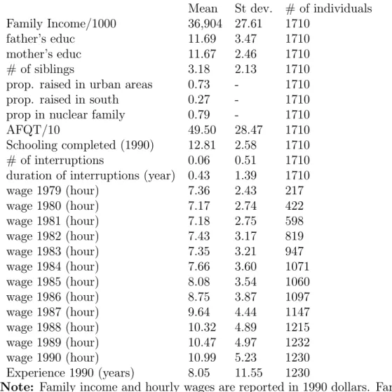
The sample used in the analysis is extracted from the 1979 youth cohort of the T he National Longitudinal Survey of Y outh (NLSY). The NLSY is a nationally representative sample of 12,686 Americans who were 14-21 years old as of January 1, 1979. After the initial survey, re-interviews have been conducted in each subsequent year until 1996. In this paper, we restrict our sample to white males who were age 20 or less as of January 1, 1979. We record information on education, wages and on employment rates for each individual from the time the individual is age 16 up to December 31, 1990.
The original sample contained 3,790 white males. However, we lacked infor-mation on family background variables (such as family income as of 1978 and parents' education). We lost about 17% of the sample due to missing informa-tion regarding family income and about 6% due to missing informainforma-tion regarding parents' education. The age limit and missing information regarding actual work experience further reduced the sample to 1,710.
Descriptive statistics for the sample used in the estimation can be found in Table 1. The education length variable is the reported highest grade completed as of May 1 of the survey year and individuals are also asked if they are currently enrolled in school or not.19 This question allows us to identify those
individ-uals who are still acquiring schooling and therefore to take into account that education length is right-censored for some individuals. It also helps us to iden-tify those individuals who have interrupted schooling. Overall, the majority of young individuals acquire education without interruption. The low incidence of interruptions (Table 1) explains the low average number of interruptions per in-dividual (0.22) and the very low average interruption duration (0.43 year) . In our sample, only 306 individuals have experienced at least one interruption. This represents only 18% of our sample and it is along the lines of results reported in Keane and Wolpin (1997).20 Given the age of the individuals in our sample, we
assume that those who have already started to work full-time by 1990 (94% of our sample), will never return to school beyond 1990. Finally, one notes that the number of interruptions is relatively small.
Unlike many reduced-form studies which use proxies for post-schooling labor market experience (see Rosenzweig and Wolpin), we use actual labor market experience. Actual experience accumulated is computed using the fraction of the year worked by a given individual. The availability of data on actual employment rates allows use to estimate the employment security return to schooling.
19This feature of the NLSY implies that there is a relatively low level of measurement error
in the education variable.
20Overall, interruptions tend to be quite short. Almost half of the individuals (45 %) who
experienced an interruption, returned to school within one year while 73% returned within 3 years.
The average schooling completed (by 1990) is 12.8 years. As described in Belzil and Hansen (2000), it is clear that the distribution of schooling attainments is bimodal. There is a large fraction of young individuals who terminate school after 12 years (high school graduation). The next largest frequency is at 16 years and corresponds to college graduation. Altogether, more than half of the sample has obtained either 12 or 16 years of schooling. As a consequence, one might expect that either the wage return to schooling or the parental transfers vary substantially with grade level. This question will be addressed below.
Table A1 - Descriptive Statistics
Mean St dev. # of individuals Family Income/1000 36,904 27.61 1710
father's educ 11.69 3.47 1710
mother's educ 11.67 2.46 1710
# of siblings 3.18 2.13 1710
prop. raised in urban areas 0.73 - 1710
prop. raised in south 0.27 - 1710
prop in nuclear family 0.79 - 1710
AFQT/10 49.50 28.47 1710
Schooling completed (1990) 12.81 2.58 1710
# of interruptions 0.06 0.51 1710
duration of interruptions (year) 0.43 1.39 1710
wage 1979 (hour) 7.36 2.43 217 wage 1980 (hour) 7.17 2.74 422 wage 1981 (hour) 7.18 2.75 598 wage 1982 (hour) 7.43 3.17 819 wage 1983 (hour) 7.35 3.21 947 wage 1984 (hour) 7.66 3.60 1071 wage 1985 (hour) 8.08 3.54 1060 wage 1986 (hour) 8.75 3.87 1097 wage 1987 (hour) 9.64 4.44 1147 wage 1988 (hour) 10.32 4.89 1215 wage 1989 (hour) 10.47 4.97 1232 wage 1990 (hour) 10.99 5.23 1230 Experience 1990 (years) 8.05 11.55 1230
Note: Family income and hourly wages are reported in 1990 dollars. Family income is measured as of May 1978. The increasing number of wage observations is explained by the increase in participation rates.