HAL Id: hal-00959373
https://hal.archives-ouvertes.fr/hal-00959373
Submitted on 14 Mar 2014
HAL is a multi-disciplinary open access
archive for the deposit and dissemination of
sci-entific research documents, whether they are
pub-lished or not. The documents may come from
teaching and research institutions in France or
abroad, or from public or private research centers.
L’archive ouverte pluridisciplinaire HAL, est
destinée au dépôt et à la diffusion de documents
scientifiques de niveau recherche, publiés ou non,
émanant des établissements d’enseignement et de
recherche français ou étrangers, des laboratoires
publics ou privés.
Quasi-static liquid-air drainage in narrow channels with
variations in the gap
Sandrine Geoffroy, Franck Plouraboué, Marc Prat, Olivier Amyot
To cite this version:
Sandrine Geoffroy, Franck Plouraboué, Marc Prat, Olivier Amyot. Quasi-static liquid-air drainage in
narrow channels with variations in the gap. Journal of Colloid and Interface Science, Elsevier, 2006,
vol. 294, pp. 165-175. �10.1016/j.jcis.2005.07.008�. �hal-00959373�
Quasi-static liquid–air drainage in narrow channels with
variations in the gap
S. Geoffroy, F. Plouraboué
∗, M. Prat, O. Amyot
Institut de Mécanique des Fluides de Toulouse, UMR CNRS-INPT/UPS 5502, Av. du Professeur Camille Soula, 31400 Toulouse, France
Abstract
This paper studies the shape of an air bubble quasi-statically flowing in the longitudinal direction of narrow channels. Two bottom topogra-phies are treated, i.e., linear and quadratic variations of the gap along the transverse direction. This work analyses the main characteristics of the gas–liquid interface with respect to the wedge aspect ratio. From the convergence of asymptotic, numerical and experimental analyses, we found simple dependences for the finger width and total curvature as a function of channel aspect ratio. These results provide simple and general expressions for the pressure drop needed to overcome capillary forces and push the air finger inside the channel.
Keywords: Drainage; Hele–Shaw; Singular; Capillarity; Microfluidic; Asymptotic; Thin films
1. Introduction
When uniformly pushing a wetting liquid with air (a non-wetting fluid) inside a channel, the air–liquid interface reaches a steady state after a transient regime. Such drainage process has a long history starting from Bretherton’s analysis of a long bubble motion inside a tube [1], while a simi-lar two-phase interface motion inside a Hele–Shaw cell has been revisited by Park and Homsy[2]. These seminal con-tributions focused on a flow regime for which the capillary number is extremely small. In similar flow regimes, more complex channel shapes were studied by Wong et al. who analysed either the static shape[3,4]or the dynamical behav-iour of the thin films left behind during the interface motion
[5,6]. These studies have shown that geometrical character-istics of the channels control the interface static shape[3,4]
as well as the dynamics of the thin fluid films[5]. To be more precise, the static interface shape is a prerequisite for under-standing dynamical behaviour[4,5].
* Corresponding author.
E-mail address:franck.plouraboue@imft.fr(F. Plouraboué).
This paper concentrates on narrow channels for which the aspect ratio between one dimension with respect to the two others is small. More precisely, given the maxi-mum gap h0 of the narrow channel and its total width 2ℓ,
we have focused on large aspect-ratio channels for which h0/ℓ≡ ǫ ≪ 1. These channels nevertheless differ from
sim-ple Hele–Shaw cells for they present spatially variable gaps (seeFig. 1). In the following we will call “linear channel” a channel for which the transverse gap varies linearly along the channel span as displayed inFig. 1a, while we will call “quadratic channel” every channel for which the transverse gap is locally quadratic at the centre of the transverse direc-tion, as displayed inFig. 1b (we will, for example, specifi-cally study a cosine profile in the experimental Section3). Non-intuitively, those simple topographical variations dras-tically change the properties of the static bubble shape, as will be detailed later in this introduction. In our case, the static shape depends on the channel aspect ratio ǫ while in the case of Hele–Shaw cell the static bubble interface shape is a ring, whose radius only depends on the gas volume and not on the Hele–Shaw aspect ratio (unless the bubble fills the span of the Hele–Shaw cell).
Fig. 1. (a) Perspective view of a sketch of the experimental linear narrow channel. The air bubble is entering from one side of the channel, while the liquid is pumped out from the other side. (b) The same conventions for a quadratic narrow channel.
To the best of our knowledge, quasi-static two-phase flows in this class of channel have not been studied yet, although they present a variety of interests [7]. First, they permit simple and precise experimental observations of the liquid–gas interface with direct optical methods. Secondly, the capillary pressure associated with a narrow channel can be rather large, for it is mainly dominated by the smallest channel dimension. This striking property of narrow chan-nels should receive particular emphasis in the context of im-bibition process[8]where the liquid first invades the chan-nel’s narrow corners. In this case, the narrower the channel, the larger the capillary pressure and the higher the imbi-bition velocity. The third interesting feature about narrow channels is that the static capillary shape determination turns out to be a new singularly perturbed problem. As a matter of fact, this paper describes how a two-dimensional study of the liquid–air interface finger inside a narrow channel leads to a singular perturbation problem associated with the channel’s aspect ratio small parameter ǫ, whereas the capillary pertur-bation problem can be considered as regular in this context.
Hence, we study the static shape interface of an air finger very slowly moving at velocity U in a perfectly wetting oil of dynamic viscosity µ inside a confined channel, as depicted inFig. 1.
In this limit, under perfectly wetting conditions, the gas– liquid interface confined between two solid surfaces dis-plays three distinct regions—a constant thin-film region in the vicinity of solid surfaces (region I,Fig. 2a), a meniscus region associated with the liquid–gas interface (region II,
Fig. 2a) and the clear original wetting fluid region (re-gion IIIl,Fig. 2a). These three regions are associated with
different dominant forces [1]. In region I, viscosity forces are dominant, because the curvature of the interface becomes equal to zero. In region II, capillary forces associated with the liquid–gas surface tension γ are dominant: the liquid– gas interface has a quasi-static quadratic shape that is locally controlled by perfectly wetting boundary conditions at the solid surface. In the third region, IIIl, the fluid flow is again
dominated by viscosity, so that the liquid flow field displays a simple local parabolic profile. The identification of these regions and their related dominant forces has provided the correct scalings for the characteristic dimensions, flow and pressure[1,2]. When the viscosity ratio between the gas and the liquid is considered negligible, these scalings are given using a single non-dimensional small parameter: the
cap-Fig. 2. (a) Lateral view of the bubble shape in the (O, x, z) plane. The origin of coordinates is taken at the bubble tip O. (b) Top view of the bubble shape in the (O, x, y) plane where the bubble horizontal position is denoted y(x).
illary number Ca= µU/γ . The perturbation expansion in this small parameter of this problem is known to be singular, so that matched expansion techniques are needed to relate the interface curvature in the static meniscus region II to thin-film region I. In the case of two-phase flows in a Hele– Shaw cell such matching shows that the thin-film thickness δ left behind the displaced meniscus asymptotically varies as δ= 1.337h0Ca2/3, where h0is the Hele–Shaw cell
thick-ness.
Park and Homsy have found corrections to this formula from a double asymptotic expansion in the small parameter Ca1/3 and the aspect ratio between the interface transver-sal modulation w and the Hele–Shaw gap that we shall not discuss here. But, we shall extensively use the relation they have derived for the pressure drop between regions IIIg and
IIIl. Considering small transversal variations of the interface
along the longitudinal coordinate x, x= y−1(y)≡ g(y), Park and Homsy have focused on situations where dg/dy∼ O(ǫ′)≪ 1, where ǫ′ is the ratio between the Hele–Shaw half-width h0/2 and the transversal interface variations w,
ǫ′= h0/2w. In this case, they have been able to derive an
O(ǫ′ 2) correction to the pressure drop between the gas in region IIIgand the liquid in IIIlthat reads
Pg− Pl= 1P (1) = γµ 2 h0 (1+ 3.80 Ca2/3)−π 4 d2g dy2 ¶ .
The pressure needed to push the gas inside the channel in-creases with the capillary number to the power of 2/3 due to the viscous dissipation in the liquid films between re-gions I and II. This O(Ca2/3)term is spatially uniform in regions IIIg and IIIl. There is moreover an additional term
which is the above mentioned O(ǫ′ 2)correction that comes from the interface curvature in the (x, y) plane, expressed here in dimensional form. Further generalisation has been
discussed by other authors such as[9–11]who considered a confined bubble in a Hele–Shaw type situation. When the (x, y) plane interface slope is not small, it has been shown that the additional term is indeed the in-plane inter-face curvature multiplied by π/4 [9–11]. Moreover, in the case where the interface displacements are not locally per-pendicular to the interface one should consider the normal velocity Unof the air–liquid interface so that a normal
capil-lary number Can= µUn/γmust be used instead of Ca in(1)
[9–11]. Reinelt also found an additional perturbative term to the above pressure drop relation associating the viscous capillary dissipation and the in-plane curvature [9,10]. Fi-nally, it is also possible to generalise the results obtained by Park and Homsy, Reinelt, and Burgess and Forster to Hele– Shaw cell geometries with quasi-parallel walls[12]. One can summarise this discussion by rewriting the pressure drop be-tween regions IIIgand IIIl as
1P = γ µ 2 h(y)¡1 + 3.80 Ca 2/3 n ¢ (2) −µ π 4 − 4.07 Ca 2/3 n ¶ d2y dx2 1 (1+ (dy/dx)2)3/2 ¶ . It should be borne in mind that this relation holds in the limit of vanishing capillary number, so that higher-order capil-lary corrections O(Ca, Ca4/3)should be expected when the interface velocity is increased. In the following we shall con-centrate on the limit of very small capillary number Ca≪ 1, so that we shall not consider these higher-order corrections. In the frame of this approximation (x, y) variations of the pressure field are not considered for they are of O(Ca) (see, for example,[11]). Hence the pressure in the liquid and in the gas are spatially uniform when only O(Ca2/3) correc-tions are included. Hence the pressure drop between the gas and the liquid is also uniform. The interface curvature adapts its shape so as to respond to the dynamical capillary varia-tions associated with the in-plane interface small variavaria-tions. At this point, this paper will neither discuss the establish-ment of the asymptotic pressure drop relation(2) any fur-ther nor will it discuss its relation with thin liquid viscous films along the solid surfaces. It will merely describe the liquid–air interface from its two-dimensional shape y(x)— see Fig. 2b—in the (x, y) plane of a narrow channel, and its relation to the channel geometrical properties. Moreover, this paper mainly focuses on regimes in which gravity forces have no influence. As previously mentioned, the channels that are considered in this study present slow variations in the gap. Even small, those variations control the static shape that differs from those obtained in a simple Hele–Shaw cell. Since the capillary statics problem means constant mean cur-vature for the interface, the question is how the interface is geometrically controlled by the channel shape. One should then realise that the gap dimension along the z direction is always much smaller than the channel dimensions in x and y directions. Hence, small variations of the gap lead to im-portant effects on the mean curvature, since it is inversely
proportional. Those small gap variations are indeed equili-brated by large interface curvature variations in the (x, y) plane (the leading-order 2/ h0term just adds a constant
in-terface pressure drop whose contribution to the static shape is null). This is why the static shape drastically differs, in our case, from the simple “ring bubble” of the Hele–Shaw cell. A more subtle effect comes from rapid in-plane variations of the interface near the channel longitudinal axis of symmetry. In a very narrow region near the bubble tip, when the dis-tance to the tip is closer than the local gap thickness, the x, y plane curvature gets much larger than in other regions. This leads to a curvature boundary layer at the bubble tip, which then needs to be analysed.
The most original contribution of this work is then proba-bly related to the fact that the in-plane problem has a sin-gular asymptotic behaviour associated with this curvature boundary layer at the bubble tip as ǫ→ 0. This geometri-cally driven singularity of the interface in-plane problem is already governing the quasi-static limit Ca→ 0 of the in-terface shape. This is why this quasi-static problem is first studied in Section2. The next section investigates the com-parison between experimental and theoretical quasi-static shape analyses. Finally, we analyse capillary corrections to the quasi-static problem. From(2)the in-plane problem ob-viously admits a regular asymptotic expansion in Ca2/3that is investigated in the last section (Section4.1).
2. Quasi-static analysis
Before leaving the reader to a more detailed analysis of the problem, we would like to outline here the main phys-ical ingredients of this geometrphys-ically driven singular static shape. In the limit Ca→ 0,(2)shows that the pressure dif-ference between the gas and the liquid is spatially uniform. Then, the interface curvature is uniform. The static inter-face shape problem is thus a free-boundary value problem associated with a constant mean curvature. The unknown curvature is fixed by the channel shape, so that the final cur-vature position y(∞) of the air finger leads to a curvature κ0= 2/h(y(∞)) which is exactly identical to the curvature at the finger tip origin O—seeFig. 2. The curvature at the point O is the sum 2/ h0+ 1/R0where R0 is the in-plane
radius of curvature at the origin. Depending on the channel shape dependence with ǫ at the origin O, different typical scales can be found. Let us first introduce the length-scale associated with the final interface position y(∞). The natural length-scale in the transverse dimension is ℓ, but y(∞) is much smaller than ℓ because the channel is nar-row. Hence, y(∞) is some intermediate dimension between h0 and ℓ. Let us then introduce this intermediate
length-scale w so that w= ǫαℓ, with 0 < α < 1, so that y(∞) ∼ w ∼ ǫαℓ. This scaling thus gives the in-plane curvature
at the origin from 1/R0∼ 2/h(y(∞)) − 2/h0. This reads
for a linear channel (see (7)for the asymptotic derivation) 2/ h(y(∞)) − 2/h0∼ ǫα/ h0, so that R0∼ h0ǫ−α. While
for a quadratic channel 2/ h(y(∞)) − 2/h0∼ ǫ2α/ h0, this
leads to R0∼ h0ǫ−2α. At the same time, far from the
ori-gin, the longitudinal length-scale variations along x are also described by w, so that x ∼ ǫαℓ∼ h0ǫα−1. Far from the
origin, the interface slope is small so that the in-plane cur-vature is given by the second derivative of the transverse shape 1/R∼ y(∞)/x2∼ ǫ1−α/ h0. Equating the scalings of
Rand R0gives the value for α for different geometries, i.e.,
−α = α − 1 ⇒ α = 1/2 for a linear shape and −2α = α − 1 ⇒ α = 1/3 for a quadratic shape.
Let us now turn to the length-scales associated with the interface rapid variations near the origin. From the problem symmetries, the shape of the interface is quadratic. When the transverse shape y0 is much smaller than w, so that y0∼
ǫw∼ h0ǫα, the quadratic tip shape at the origin gives the
corresponding rapidly varying longitudinal length-scale ξ∼ y20/R0∼ h0ǫ3α for the linear shape associated with R0∼
h0ǫ−α which is much smaller than h0. The ratio between
these inner typical longitudinal variations to the outer ones w is, in this case, ξ /w∼ h0ǫ3α/ h0ǫα−1∼ ǫ2α+1, so that
given α= 1/2 leads to ξ/w ∼ ǫ2the ratio between the inner and the outer length-scales.
In the case of quadratic shape, ξ ∼ y20/R0∼ h0ǫ4α, so
that given α= 1/3 leads to the same result, ξ/w ∼ ǫ2. Hence, in both cases, when the transverse shape dimension y0 is much smaller than the outer scale w, y0∼ ǫw, the
quadratic tip-shape at the origin leads to an even smaller as-sociated longitudinal variations ξ ∼ ǫ2w. These variations
have large slope of the order y0/ξ ∼ ǫ−1, with small
ra-dius of curvature R0∼ h0ǫ−1/2 for linear shape or R0∼
h0ǫ−1/3for quadratic shape. These geometrical features give
the main ingredients of the problems that are subsequently solved in Sections2.3.1 and 2.3.2.
From this analysis, one can now deduce the proper non-dimensionalisation of the problem. The transverse direction y is then normalised by the transverse channel width ℓ while the vertical gap h is non-dimensionalised by its maxi-mum h0. The longitudinal direction x and the finger width y
are non-dimensionalised by the same length-scale w, associ-ated with the asymptotic finger width. As mentioned above, w satisfies an intermediate scaling w= ℓǫα, with α= 1/2
for a linear channel and α= 1/3 for a quadratic one. Any generalisation to higher-order channel shape trivially fol-lows from the presented results. The non-dimensionalisation of variables related to the channel geometry can be sum-marised using the following tilde variables:
(x, y, z, ξ, w, y, h)
(3) = (w ˜x, ℓ ˜y, h0˜z, w ˜ξ, ℓǫα, w˜y, h0˜h).
It should nevertheless be borne in mind that the intermedi-ate length-scale w is the correct length-scale to describe the quasi-static capillary width of the finger, but not the capillary corrections coming from non-zero capillary number. Hence, in the following we will look for asymptotic solutions for the air–liquid finger width as a regular expansion in the capillary
number that will be denoted with an upper index:
(4) ˜y = ˜y0+ Ca2/3ǫ−α˜y1+ O(Ca, Ca4/3).
The first term corresponds to the quasi-static shape whose typical length-scale is w so that it is obviously of O(1) when non-dimensionalised by w. The second term describes a capillary correction which scales as the channel width ℓ, so that the non-dimensionalisation(3) makes this term O(Ca2/3ǫ−α).
The first quasi-static term is examined analytically in Section 2.1. This terms is associated with a classic non-linear static capillarity problem which admits few exact so-lutions[13]. Hence, rather than focusing on the finger shape, the Section2.1rather concentrates on finding the properties of the asymptotic finger width y0(∞), for different channel shapes. Yet the complete shape cannot be computed analyti-cally, and it will be computed numerically in Section2.2. In Section2.3we shall seek an asymptotic solution associated with the channel aspect ratio small parameter ǫ. Indeed, Sec-tion2.3will only investigate the leading-order approxima-tion of this first term, which satisfies a singularly perturbed problem the precise formulation of which depends on the channel shape. Let us now define the non-dimensionalised pressure ˜P using the usual capillary pressure ˜P = h0P /2γ
associated with the maximum channel aperture h0. Equation
(2)can then be expressed in non-dimensional form 1 ˜P= 2 ˜h( ˜y, ǫ)¡1 + 3.8 Ca 2/3 n ¢ − ǫ1−αd 2 ˜y d˜x2 1 (1+ (d ˜y/d ˜x)2)3/2 µ π 4 − 4.07 Ca 2/3 n ¶ , (5) Can= Ca d˜y d˜x 1 (1+ (d ˜y/d ˜x)2)1/2,
while the non-dimensional gap ˜h(˜y, ǫ) is now depending on the small parameter ǫ which needs to be expanded for spe-cific geometries. As explained earlier, keeping with a small capillary number approximation the pressure is spatially uni-form, so that the interface adapts its shape to respond to the small interface dynamical displacements. This section con-centrates on the zero capillary number limit of(5)for which the non-dimensional liquid–gas interface, ˜y0, in this limit, displays a constant unknown total curvature˜κ0,
−ǫ1−απ 4 d2˜y0 dx2 1 (1+ (d ˜y0/dx)2)3/2+ 2 ˜h( ˜y0, ǫ) (6) = 2 ˜h( ˜y0(∞))= ˜κ 0,
which is equal to the radius of curvature associated with the finger width ˜y0(∞) as x tends to infinity. This formulation
of the static shape problem displays the generic property of a singularly perturbed problems, for which a small parameter multiplies the highest derivative. Hence, the finger-tip rapid variations of the plane curvature are localised in some in-ner boundary layer that shrinks with ǫ, while the smooth
Fig. 3. Numerical computation (continuous line) and asymptotic prediction (dotted line) of the finger width y0(∞) normalised by the channel width ℓ. (a) Linear channel for which the asymptotic behaviour(21)is y0(∞)/ℓ =√ǫπ/4. (b) Sinusoidal channel for which the asymptotic behaviour(30)is y0(∞)/ℓ = (3πǫ/16)1/3.
finger width variations are associated with the outer inter-mediate length-scale w.
2.1. Finger width ˜y0(∞)
2.1.1. Linear wedged tripod
We consider here the case where h(y)= h0(1− |y|/ℓ),
so that
(7) ˜h = 1 − | ˜y| = 1 −√ǫ| ˜y|.
Equation (6) can easily [13] be integrated, from ˜x = 0 where ˜y0(0)= 0 and d ˜y0(0)/d˜x → ∞ to infinity where d˜y0(∞)/d ˜x = 0, so that (8) −π 4ǫ+ 2 ln¡1 − √ ǫ˜y0(∞)¢ + 2 √ ǫ˜y0(∞) 1−√ǫ˜y0(∞)= 0.
We then have an implicit solution for the finger width˜y0(∞) as a function of the aspect ratio h0/ℓ= ǫ. Inverting(8)it is
possible to find an explicit relation between those quantities, (9) ˜y0(∞) = ǫ−1/2¡1 − e¡
W (−1,−e(−πǫ/8+1))+πǫ/8+1¢
¢,
where W is the−1 branch of the Lambert’s W-function[14].
Fig. 3a displays the behaviour of the asymptotic finger width y0(∞) versus the aspect ratio. As expected, this figure shows that the finger asymptotic width y0(∞) shrinks as the aspect ratio ǫ of the linear edge decreases. The concave shape of the curve when ǫ≪ 1 is related to the leading-order √ǫ scaling that can be obtained from a Taylor ex-pansion of(9). This indicates that y0(∞)/ℓ has a less than linear dependence on ǫ so that the width shrinkage is self-consistently always larger than the meniscus radius which precisely scales as ǫ. This scaling will be specifically stud-ied in Section2.3.1.
2.1.2. Quadratic narrow channel
We now turn to the case where h(y)= h0cos(
√ 2y/ℓ). Here again the integration of Eq.(6) gives an implicit de-pendence for the asymptotic finger width on the aspect ratio:
π 4ǫ+
√
2 ln¡√2ǫ1/3
˜y0(∞) + tan¡√2ǫ1/3˜y0(∞)¢¢
(10) − 2ǫ
1/3˜y0(∞)
cos(√2ǫ1/3˜y0(∞)) = 0.
This equation cannot be made analytically explicit, but it can easily be solved numerically.Fig. 3b sketches the varia-tions of the asymptotic width versus the aspect ratio. Here again, the width shrinkage, when the aspect ratio varies, is self-consistently always larger than the meniscus radius. Moreover, as will be further investigated in Section 2.3.2, the behaviour of the asymptotic width with the aspect ratio is different from those obtained in the case of a linear chan-nel.
To conclude this section it should be noted that an explicit expression of the finger asymptotic width could be obtained from a simple Taylor expansion of implicit relations(8) and (10)with the small aspect ratio parameter ǫ. We do not give them here, but they will be obtained in a similar way in Sec-tion2.3in relations(21) and (30).
2.2. Numerical computation of the quasi-static air–liquid shape ˜y0
In general, the analysis of the complete shape of the liquid–gas interface resulting from capillary equilibrium ne-cessitates numerical computation[13]. As a matter of fact, Eq. (6) defines a free-boundary value problem associated with a perfectly wetting air–liquid interface presenting an a priori unknown constant mean curvature ˜κ0. For the spe-cial class of problems examined in this paper, the interface shape can be obtained from the numerical integration of the non-linear ordinary differential equation (6). This can be easily done with a Runge–Kutta method, after dealing with the singularity at the origin. Let us first define an interesting variable change for which, rather than focus-ing on the longitudinal variation of the ffocus-inger transversal width y= y0(x), we consider the transversal variation of its length x= ( ˜y0)−1(y)≡ g(y). This variable change is interesting from a numerical point of view, since the in-verse of y0(x)is not singular any more in the vicinity of the finger tip. Let us now, consider the standard variable change between the local slope dg/dy and the tangent an-gle θ , tan θ = dg/dy. Next, considering the usual vector-ial representation for the shape-slope variable g= (g, θ), it is easy to reformulate the second-order differential
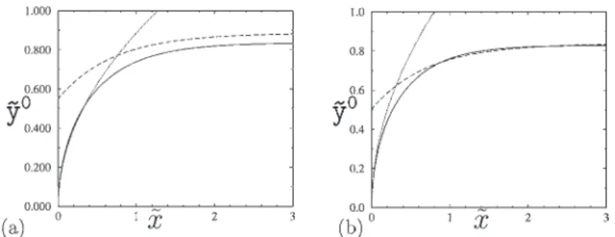
equa-Fig. 4. Numerical computation of in-plane interface shape˜y0(x)in continuous lines for two channels of aspect ratio ǫ= 10−2. Dotted lines represent the inner asymptotic behaviour, dashed lines the exponential decay of the outer solution. (a) Linear channel; (b) sinusoidal channel.
tion(6)as (11) dg dy = µ tan θ, 4 πcos θ µ 2 h(y0(∞))− 2 h(y) ¶¶ ,
with associated initial conditions g(0)= (0, 0). Its non-dimensional formulation associated with ˜g = ( ˜g, θ) = (g/w, θ )reads (12) d˜g d˜y = µ ǫ−αtan θ, 4 ǫπcos θ µ 2 ˜h( ˜y0(∞))− 2 ˜h( ˜y) ¶¶ , with associated initial conditions g(0)= (0, 0). One should note that we have kept dimensional variables in the formu-lation of the problem, since the numerical solution later on will be compared with dimensional experimental measure-ments. The non-dimensional formulation of (11) is never-theless straightforward. The a priori unknown asymptotic width ˜y0(∞) can either be found from solving the implicit equations (8), (10), or by directly implementing a shoot-ing method out of the Runge–Kutta integration of Eq.(11). A fourth-order constant integration step procedure rapidly converges (with a few thousand steps) to a highly precise fin-ger shape determination (relative error smaller than 10−7). The resulting integration has led to Fig. 4 in the case of the linear and sinusoidal channels introduced in the previ-ous section. From this figure, it can be observed that af-ter an initial stage of rapid variation, the in-plane curva-ture reaches a smooth longitudinal decay. The size asso-ciated with those rapid curvature variations is small, com-pared to the finger width. It will be identified as a curvature boundary layer in Section4. Moreover, the slow longitudi-nal decay has been previously identified as being exponen-tial in[15], using another, more general, numerical method
[16]. We again find (for both geometries) an exponential decay that will be further investigated analytically in Sec-tion2.3.
2.3. Asymptotic approximation for ˜y0
2.3.1. Linear wedged tripod
In the case of the linear channel previously studied, the non-dimensional linear shape has been written in(7). Ex-panding ˜hfor positive values of ˜y in(7), it is found that − 2 ˜h( ˜y0, ǫ)+ 2 ˜h( ˜y0(∞))= 2ǫ α¡ ˜y0( ∞) − ˜y0¢
ס1 + ǫα¡ ˜y0(∞) + ˜y0¢¢ + O(ǫ3α),
which, from(5)and(4), fixes here 1− α = α, i.e., α = 1/2, and the intermediate non-dimensionalised length-scalew˜ to scale asw˜ =√ǫ, as already mentioned in the beginning of this section. Let us now look for a regular asymptotic ex-pansion with the small parameter ǫ for the quasi-static outer finger shape, that will be denoted by the capital letter˜Y0:
(13) ˜Y0 = ˜Y00+ √ ǫ˜Y0 1+ · · · .
Similarly, all the following subscript numbers will refer to such regular asymptotic expansion with the small parameter ǫ. Expansion(13)leads to the following leading-order prob-lem: (14) −π 4 d2˜Y0 0 d˜x2 1 (1+ (d ˜Y00/d˜x)2)3/2 + 2¡ ˜Y0 0− ˜Y 0 0(∞)¢ = 0.
First, we would like to find the finger asymptotic width ˜Y0
0(∞), using the same method as in Section2.1.1,
integrat-ing(14)after multiplying by d˜Y0
0/d˜x from ˜x = 0 to infinity: (15) π 4 1 q 1+ (d ˜Y00/d˜x)2 = − ˜Y00¡ ˜Y 0 0− 2 ˜Y 0 0(∞)¢.
Boundary conditions (˜Y0 0(0), d˜Y
0
0(0)/d˜x) have to be found
by matching the inner solution with the outer one. The outer problem complete solution can moreover be solved formally using the variable change previously introduced in Section2.2. This, in turn, leads to the simpler problem(16)
to solve, (16) π 4 cos θ0 dθ0 d˜Y0 0 + 2¡ ˜Y0 0− ˜Y 0 0(∞)¢ = 0
where θ0 is related to the inverse of the shape function
˜
G0= ( ˜Y00)−1by tan θ0= d ˜G0/d˜Y00. A first integral form of
the solution of(16)is (17) θ0¡ ˜Y00¢ − θ0(0)= − arcsin µ 4 π˜Y 0 0¡ ˜Y00− 2 ˜Y00(∞) ¢ ¶ .
The boundary condition to be applied to the outer slope at ˜x = 0 has to be found from matching the inner solution. As mentioned in the introduction of this section, the related in-ner problem involves a new inin-ner variable ˜ξ= ˜x/ǫ2, which is associated with rapid variations of the curvature. We can
then look for a regular expansion of the inner solution in this new variable:
(18) ˜y0= ˜y00( ˜ξ )+ ǫ ˜y01( ˜ξ )+ · · · .
Substituting this expansion for ˜y in (5) one finds that the leading order ˜y00 has to be constant, with the associated
boundary condition ˜y00(0)= 0. Then, this constant is zero,
and the first non-zero term of the inner problem is˜y01, which
fulfils (19) −π 4 d2˜y1 d ˜ξ2 1 (d˜y1/d ˜ξ )3 = 2 ˜Y00(∞).
The solution of (19) associated with boundary condition y01(0)= 0 is (20) ˜y01( ˜ξ )= π 4 q ˜ξ ˜Y0 0(∞) .
Then, matching the outer with inner solutions leads, to lead-ing order, to boundary conditions ˜G0(0)= 0 and d ˜G0(0)/
d˜Y0
0= 0 = θ0(0). From(15), those boundary conditions
ap-plied to the outer solution lead to the asymptotic leading-order finger width ˜Y0
0(∞) =
√
π/4. This result can be com-pared with the computation of Section2.1.Fig. 3a displays the ratio of the finger asymptotic width to the channel width versus the aspect ratio, as well as the comparison with its leading-order asymptotic behaviour for the dimensionalised finger width, (21) y00(∞) ℓ = ˜Y 0 0(∞) √ ǫ=r π 4ǫ,
showing a very nice agreement as ǫ→ 0. Hence the inner solution reads, to O(ǫ2),
(22) ˜y0= ǫ r ˜ξπ 4 = r ˜xπ 4,
while the inverse shape of the outer solution ˜G0 can be
deduced analytically from integrating (17). The integra-tion leads to a rather cumbersome expression, the far field √
π/4− ˜Y00≪ 1 behaviour of which being
(23) ˜ G0¡ ˜Y00¢ ∼ π 4 √ 2 2 arctanh µs 2 −( ˜Y00)2+ 2 ˜Y00+ 1 ¶ .
This behaviour leads to a simple exponential decays for the outer finger shape as ˜x ≫ 1:
(24) r π 4 − ˜Y 0 0(˜x) ∼ exp¡− √ 2˜x¢.
Results(22) and (24)are compared with the numerical solu-tion of(5)in the case of a linear channel inFig. 4a, showing an excellent matching with the numerical results of Sec-tion2.2. The approximated inner behaviour obtained in(22), and the approximated outer region which displays an expo-nential decay y0(x)/w=√π/4− 0.335 exp(−√2x/w)+ O(ǫ)for x≫ w as described in(24), are compared with the
full numerical solution. Very similar results have been ob-tained for the far field exponential behaviour in non-confined polygonal channels by[4]and[15]. This exponential decay could be straightforwardly obtained from linearising(14)in the limit of a small low interface slope.
2.3.2. General quadratic shape
Let us now turn to the case of a general quadratic shape for which the channel depth has a maximum at h(0)= h0.
Expanding the shape in the vicinity of the maximum in di-mensionalised variables leads to
(25) h= h0− 1 2hyyy 2 +1 3hyyyy 3 + · · · .
In the previously introduced non-dimensional quantities this expansion reads
(26) ˜h = 1 − ǫ2α
˜y2+ ǫ3αβ˜y3+ · · · ,
where again ǫ = h0/ℓ=ph0hyy/2 and β= 2hyyy/3h2yy.
In the following, we will nevertheless concentrate on the leading-order quadratic term, and neglect the contribution of higher-order terms in the description of the profile geometry. As previously examined, this leads to the vertical curvature expansion −2 ˜h+ 2 ˜h( ˜y(∞))= 2ǫ 2α¡ ˜y(∞)2 − ˜y2¢ + ǫ4α¡ ˜y(∞)4 + ˜y4¢ + · · · ,
which, in turn, from(5)leads to 1− α = 2α, i.e., α = 1/3, and the intermediate length-scalew˜ associated with the non-dimensionalised finger width to scale as w˜ = ǫ1/3. Follow-ing the same steps as in the previous section, we seek for a regular asymptotic expansion of the outer solution as a func-tion of ǫ1/3, the leading order of which fulfils
(27) −π 4 d2˜Y0 0 d˜x2 1 (1+ (d ˜Y00/d˜x)2)3/2 + 2¡¡ ˜Y0 0 ¢2 − ˜Y00(∞) 2 ¢ = 0. The boundary conditions applied to this outer problem are also given from matching the inner problem with the outer one. Seeking for the same regular expansion as(18)for the inner problem, the leading order ˜y1now fulfils
(28) −π 4 d2˜y01 d ˜ξ2 1 (d˜y01/d ˜ξ )3 = 2 ˜Y00(∞) 2,
the solution of which, associated with boundary condition ˜y01(0)= 0, is (29) ˜y01(ξ )= π 4 q ˜ξ ˜Y0 0(∞)2 .
Matching the inner and outer solutions leads to the same boundary conditions for the outer as in previous section,
˜
(27)from ˜x = 0 to infinity then leads to the outer asymp-totic shape width ˜Y0
0(∞) = (3π/16)1/3, so that (30) y00(∞) ℓ = ˜Y 0 0(∞)ǫ 1/3 =µ 3π 16ǫ ¶1/3 .
This result nicely fits the numerical computation of Sec-tion2.2for the sinusoidal channel depicted inFig. 3b. There-fore, the inner leading-order finger shape finally reads, in the case of a quadratic channel profile,
(31) ˜y =µ π 4 ¶1/3µ 4 3 ¶2/3 ǫ q ˜ξ =µ π 4 ¶1/3µ 4 3 ¶2/3√ ˜x.
Following the same lines as in the previous section, the ex-plicit computation of the leading-order inverse ˜G0= ( ˜Y00)−1
can be obtained analytically, from which the asymptotic be-haviour as (3π/16)1/3− ˜y ≪ 1, or similarly ˜x ≫ 1, leads to the same exponential decay for the finger shape:
˜Y0 0(∞) − ˜Y 0 0(˜x) = µ 3π 16 ¶1/3 − ˜Y00(˜x) (32) ∼ exp¡−√2˜x¢.
Both results (31) and (32) are compared to the interface shape numerical computation inFig. 4b. The approximated inner behaviour obtained in (31) and the outer exponen-tial decay y0(x)/w= (3π/16)1/3− 0.335 exp(−√2x/w)+ O(ǫ)for x≫ w described in(32)are represented.
3. Experiments
Some channels have been built in two steps. First, poly-meric material has been carved with an automatic microma-chining device. The channel depth function h(y) has been very finely discretized, so as to permit an optimal use of the machining precision, which is equal to 10 µm in every (x, y, z) direction. The channel’s maximum depth h0 has
been chosen equal to h0= 1 mm for every channel. The
maximum depth h0 is of the same order of magnitude as
the capillary length ℓc =√γ /ρg obtained from balancing
surface tension γ with gravity acceleration g acting on the fluid volume density ρ. As a matter of fact, the surface tension between the silicon oil and air has been measured equal to γ = 21.7 mN m−1with a Langmuir–Wilhelmy bal-ance. Since the oil density is ρ= 968 kg m−3, the capillary length is equal to ℓc= 1.5 mm. Nevertheless, the influence
of gravity forces should remain small since the Bond num-ber associated with the experiments is close to 0.4 [13]. Moreover, each channel has been aligned along the horizon-tal plane. This alignment has been checked from inspecting the symmetry of the liquid–air interface along the transverse coordinate y, as well as by checking the translational in-variance along the longitudinal coordinate x. The channels width is 2ℓ= 50 mm and their total length 15 cm. Hence the aspect ratio of the channels has been chosen equal to ǫ= h0/ℓ= 0.04. In a second step, a Plexiglas plate of 1 cm
thick is fixed on top of the carved polymeric material. Leak-age is prevented thanks to a silicon paste disposed on lateral grooves machined along the carved channel. The top plate has been fixed with equally spaced and controlled clamp-ing screws. Then, one side of the channel is open to ambient pressure, while the other side is connected to a screw-driven pump through a Plexiglas injector. The channel sits horizon-tally on a tray in which the fluid is collected. Experiments were carried out by slowly pumping out a perfectly wet-ting silicon oil. The ratio of viscous to capillary forces is given by the capillary number Ca= µv/γ , where the ve-locity is estimated from the ratio of the pumped flux q to the channel surface S=Rℓ
−ℓh(y)dy, v= qS. Two different
oils have been used during the experiments. This allowed us to change the capillary number either by getting the fluid velocity to vary or by choosing different dynamic fluid vis-cosities µ. The oil dynamic visvis-cosities have been measured with a cone viscometer equal to µ= 0.068 and 0.22 Pa s at 20◦C. A constant temperature of 22± 1◦C has been main-tained during all the experiments. The experiments were recorded with a CCD camera using a large-angle optics (the focal distance could vary from 18 to 35 mm) above the chan-nel. The images were taken at 2 frames/s with a resolution of 0.1 mm. Very low capillary numbers have been explored from 3× 10⁻³to 10−5giving no significant differences in the top view shape of the air finger inside the channels. Con-trary to the thin liquid film left behind the top horizontal plate discussed in the Introduction, the in-plane character-istics of the liquid–air interface are weakly sensitive to the capillary number. A careful analysis of the finger horizontal plane relative width y0(∞)/ℓ measured from these experi-ments displays a very small influence of the capillary num-ber in the explored range. Neither does the finger tip present any change at small capillary number.
This gives support to a quasi-static capillary equilibrium shape that we have analysed in the two previous sections. Let us first consider the comparison between the observed finger relative width y0(∞)/ℓ and the theoretical predic-tions. Hopefully, both numerical and theoretical analyses of the previous section give consistent identical result for the linear and sinusoidal channels that we have designed for our experiments. In the case of the linear channel, theoretical prediction for the finger relative width is y0(∞)/ℓ = 0.158, while experimental measurements associated with the low-est capillary number give y0(∞)/ℓ = 0.173 ± 0.002. There is thus a nice agreement up to 8%. Moreover, when stop-ping the pump, so as to observe the static interface shape, no detectable difference with the presented profile has been obtained in both cases when waiting for several hours. This time-scale is much larger than the typical capillaro-viscous relaxation of the in-plane finger shape y which is close to few seconds in our experiments, as discussed in
Appendix A. Hence,Fig. 5displays the relaxed quasi-static shape of the in-plane finger. This point should neverthe-less be taken with care, because thin films located close to the solid surfaces above and bellow the air finger have
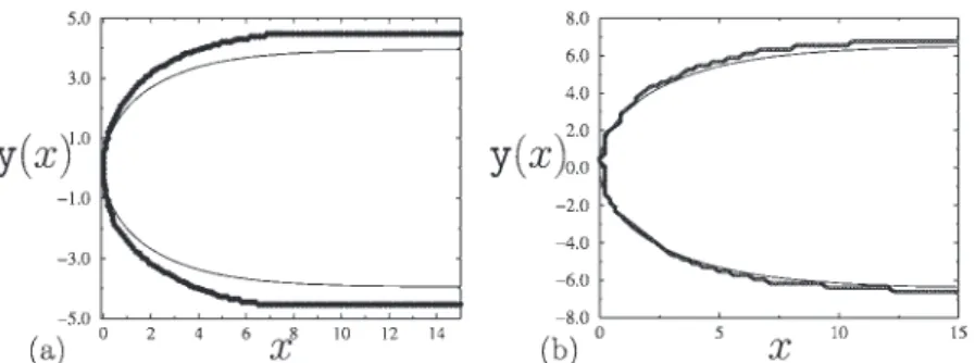
Fig. 5. Comparison between numerical computation (continuous line) and experimental measurements (circles) of in-plane interface shape y(x). Each coordi-nate is expressed in millimetres. (a) Linear channels (filled circles) are associated with Ca= 10−4. (b) Sinusoidal channels (open circles) are associated with Ca= 3 × 10⁻⁵.
very long capillaroviscous relaxation times as explained in
Appendix A. Their impact on the in-plane finger shape y is nevertheless negligible, as also shown in Appendix A. The experimental uncertainty coming from the optical pix-elisation is nevertheless smaller than the observed differ-ence between theoretical and experimental results. The ob-served mismatch should rather be associated with some dif-ferences between the ideal linear channel and its experi-mental model. A similar conclusion can be drawn in the case of the sinusoidal channel for which theory predicts y0(∞)/ℓ = 0.277, while experimental measurements give y0(∞)/ℓ = 0.28 ± 0.002, leading to less than 1% deviation. The shape of the finger tip is also interesting to com-pare with the predictions of static equilibrium obtained from numerical computation.Fig. 5displays this comparison. In the case of the linear channel, since the asymptotic width falls off by 8%, the prediction for the interface shape can not be much better. On the contrary, the comparison of the sinusoidal case shows an excellent agreement between ex-perimental measurements and numerical results. No free parameter has been used to display both comparisons, the geometrical parameters used for the numerical computation being exactly mapped to the experimental dimensions of the narrow channels.
4. Capillary corrections
4.1. First capillary corrections ˜y1
From the regular expansion of the pressure(5)it is then possible to find the O(Ca2/3)capillary correction to(4). As will be seen in the following, the capillary correction to the interface shape fulfils an ordinary differential problem which is determined by the static shape ˜y0. In Section2.2we have numerically computed the quasi-static shape ˜y0. This result could be used here to compute numerically the leading-order capillary correction˜y1.
Besides, we are more interested in the influence of the capillary correction on the finger width, so we shall restrict our analysis to an estimate of˜y1(∞) which can be computed independently from the precise knowledge of˜y0.
4.1.1. Linear wedged tripod
In the case of linear transverse variations of ˜h, the first perturbation O(Ca2/3)correction to Eq.(5)reads
−π 4 d2˜y1 d˜x2 1 (1+ (d ˜y0/d˜x)2)3/2+ 2¡ ˜y 1 − ˜y1(∞)¢ (33) = 3.8µ d ˜y 0 d˜x 1 (1+ (d ˜y0/d˜x)2)1/2 ¶2/3 .
This linear second-order ordinary equation for ˜y1is forced by ˜y0.˜y1(∞) can nevertheless be computed since we know from previous analysis that one of the boundary condition to be applied at x= 0 is 1/(d ˜y0(0)/d˜x) = 0 so that, from
(33), we deduce that ˜y1(0)− ˜y1(∞) = 3.8/2. Moreover, we know that the other boundary condition at the origin is ˜y(0) = 0 so that from (4), ˜y0(0)= ˜y1(0)= 0. Hence we find that ˜y1(∞) = −1.9.
4.1.2. General quadratic shape
The very same analysis could be applied to the quadratic shape. Hence these are the results for the first capillary cor-rection problem: −π 4 d2˜y1 d˜x2 1 (1+ (d ˜y0/d˜x)2)3/2+ 4¡ ˜y 0
˜y1− ˜y0(∞) ˜y1(∞)¢ (34) = 3.8µ d ˜y 0 d˜x 1 (1+ (d ˜y0/d˜x)2)1/2 ¶2/3 .
Using the same argument as in the previous section, we find that the far field asymptotic correction to the finger width is ˜y1(∞) = −3.8/4 ˜y0(∞) = −(3.8/4)(16/3π)1/3+ O(ǫ1/3)≃ −1.13.
4.2. Discussion
Let us first summarise the results obtained in the preced-ing analysis about the fpreced-inger asymptotic width in the case of a linear transverse shape ˜h(˜y) = 1 −√ǫ| ˜y|,
y(∞) ℓ = r πǫ 4 − 1.9 Ca 2/3 (35) + O¡ǫ, Ca, Ca4/3,√ǫ Ca2/3¢,
while in the case of a quadratic shape ˜h(˜y) = 1 − ǫ2/3˜y2, the results established in the previous section give
(36) y(∞) ℓ = µ 3π 16ǫ ¶1/3 − 1.13 Ca2/3 + O¡ǫ2/3, Ca, Ca4/3, ǫ1/3Ca2/3¢.
Hence, in both cases, the influence of the capillary effects reduces the finger width. We self-consistently qualitatively observed that increasing Ca leads to narrower finger in the experiments. From these results it is easy to estimate a capil-lary number limit for the validity of the quasi-static analysis presented in Section 2. Comparing the O(Ca2/3)capillary correction to the finger width correction in relations(35) and (36)one can find the capillary number above which the in-terface finger width will be sensitive to the capillary number variations. In the case of a linear narrow channel one finds this capillary number value to be Ca= (√ǫπ/4/1.9)3/2≃ 0.32ǫ3/4, while in the case of a quadratic channel Ca= (3π/16ǫ)1/2/(1.13)3/2≃ 0.63√ǫ. In both cases, the experi-mental aspect ratio ǫ has been chosen equal to 0.04, so that the associated capillary number value is Ca= 2.810−2for the linear channel and Ca= 1.210−1for the quadratic one. These values are worth comparing to the experimental val-ues reported in the caption ofFig. 5.
In both cases the capillary numbers were much smaller than these values, and therefore the quasi-static hypothesis should be verified.
5. Conclusion
The results presented in this paper show that small cap-illary number drainage of a wetting liquid by a gas inside a channel can be described by a quasi-static capillary equi-librium. In this limit, one may successfully compare the ob-served experimental liquid–gas interface shape with numeri-cal computation and theoretinumeri-cal analysis related to a constant curvature interface. Taking advantage of the large aspect ra-tio of the channel geometries under study, an asymptotic analysis provides general expression for the main charac-teristics of the interface as is summarised in(35) and (36). These results should moreover be easy to generalise for any transverse shape channels, following the same steps as those presented in Section4. The interface being of constant cur-vature in the quasi-static limit, the position of the finger width therefore provides the exact value of the correspond-ing curvature. It is thus easy to deduce from(2)that the pres-sure difference to be applied to push the air finger inside the channel is equal to 1P = 2γ (1 +√ǫπ/4+ 3.8 Ca2/3)/ h0
in the case of the linear channel and to 1P = 2γ (1 + (ǫ3π/16)2/3+ 3.8 Ca2/3)/ h0for a quadratic channel.
Another interesting result is that, for channels having a large aspect ratio, the interface tip exhibits rapid variations of in-plane curvature which are related to a curvature boundary layer. The boundary layer tip shape y scales with the longi-tudinal distance x as y∼√x, independently of the channel
geometry. Moreover, far from this boundary layer, the in-terface curvature reaches a smooth longitudinal variation re-gion, associated with an exponential decay, as already found in[4] and[15]. We furthermore found that this exponen-tial decay is associated with a typical length w/√2, where w/ℓ=√ǫ in the case of linear channel and w/ℓ= ǫ1/3 for a quadratic shaped channel. A complementary capillary asymptotic analysis has provided analytical bounds for the capillary number associated with the presented quasi-static results. It has been found that the capillary effects can be ne-glected when Ca≃ 0.32ǫ3/4in the case of a linear channel, and as Ca≃ 0.63√ǫin the case of a quadratic one.
The presented results are easy to adapt to more general wettability conditions where the contact angle φ is differ-ent from 0. As a matter of fact, the general case where 0 < φ < π/2 could be obtained from substituting the aper-ture gap h0by h0/cos φ, since the vertical radius of
curva-ture of the interface is modified from h/2 to h/(2 cos φ).
Acknowledgments
We thank Laurent Limat for pointing out the Park and Homsy π/4 correction to the in-plane curvature term. We also thank Arnaud Antkowiak for his expertise on matlab solvers. Finally we thank Grégory Dhoye and François Este-ban for technical support. The research presented in this pa-per is supported by GDR 2345 “Etanchéité statique par joints métalliques en conditions extrêmes” encouraged by CNES, Snecma-Moteur, EDF and CNRS. This work has been par-tially supported by PIR CNRS “Microfluidique.”
Appendix A
In this appendix we discuss the transient behaviour to the quasi-static state associated with both the thin films, that are located close to the solid surfaces above and bellow the air finger, and the interface mean position y(x, t). The analy-sis that is given here is a first simplified discussion about the complete transient problem that we will not consider in de-tail. Our objective here is mainly to extract the correct orders of magnitude for the transient viscous relaxation to occur.
First, let us recall the classical thin-film dynamic equation (see, for example,[5]). As previously discussed, the quasi-static pressure drop between the gas and the liquid is the cap-illary pressure. Considering that the viscosity ratio between the gas and the liquid is very small, the associated pressure drop in the gas is negligible compared with the one in the liq-uid. Consequently, we will take, as usual, the gas pressure as a zero reference pressure. The capillary pressure thus leads to a simple decouple expression for the quasi-static liquid pressure. Let us first consider the thin-film region, the film thickness of which will be denoted h(x, y, t). From the sim-plified expression of the mean curvature in slowly varying thin films, the liquid pressure in the film reads p= γ 1h.
The lubrication equations for the momentum x and y com-ponents can then easily be solved and lead to simple shear flow, that can be integrated to give an horizontal fluid flux
q in the film along the (x, y) plane. This fluid flux q is
proportional to the pressure gradient and the cube of the film thickness h, as usual in those Darcy-like problems, i.e.,
q= (h3/12µ)∇p. The conservation of flux then leads to the classical thin-film dynamical equation:
(A.1) ∂th+ γ 12µ∇ · (h 3 ∇1h) = 0.
One would then like to seek for the scaling of the cap-illaroviscous relaxation time of the films that will be de-noted τf. We consider x and y variations of the film to
be of the order w and the film thickness h is given by the Bretherton result h∼ h0Ca2/3. Using(A.1)and the previous
scaling w/ h0∼ ǫα−1leads to τf ∼ (h0µ/12γ )ǫ4(α−1)/Ca2.
A typical estimation using the experimental values given in Section3, with γ = 21.7 mN m−1, µ= 0.22 Pa s, h0=
10−3m, Ca= 10−4 and ǫ= 0.04 leads to values as large as τf ∼ 5 × 10⁸s for the linear channel where α= 1/2 and
τf ∼ 5 × 10⁹ s for the quadratic channel where α= 1/3.
Hence, the relaxation time for the film temporal reorganisa-tion far exceeds several weeks, so that this relaxareorganisa-tion could not be achieved in the experiments. Nevertheless, the thin-films contribution to the quasi-static bubble shape y(x) can be estimated from computing the liquid volume in the films, as compared to the liquid volume needed to displace the bubble shape y(x) position of a distance equal to the menis-cus size h0/2. For a bubble of length L and width 2w, the
liquid film volume is h0Ca2/32wL. The volume necessary
to displace the bubble at one meniscus distance is close to π/2(h0/2)2Lfor a perfect wetting condition. Hence the
vol-ume ratio is (π/16)h0/Ca2/3w= (π/16) Ca2/3ǫα−1which
gives respectively 2× 10⁻³ and 3× 10⁻³ for linear and quadratic channels. Hence, the contribution of the films to the bubble shape quasi-static position y(x) is negligible.
Finally, let us discuss the relaxation time of the interface position shape y(x, t) far from the inner curvature boundary
layer. The governing equation for the shape y(x, t) can be found in[8]and[17]and reads
(A.2) 36µ
γ ǫ ∂ty
2
= ∂x2y3.
Using the dimensional quantities given in(3), so that x∼ w and y∼ w, one can easily obtain the transient capillaro-viscous relaxation time τs for the in-plane shape y(x, t),
τs∼ (36µ/γ )h0ǫα−2. A typical estimation using the
exper-imental values given in Section3, with γ = 21.7 mN m−1, µ= 0.22 Pa s, h0= 10−3m, Ca= 10−4and ǫ= 0.04, leads
to values τs ∼ 4 s and τs ∼ 3 s for linear and quadratic
channels. Hence, the transient time for the relaxation to the quasi-static shape of the interface position shape y(x, t) is of the order of few seconds.
References
[1] F.P. Bretherton, J. Fluid Mech. 10 (1961) 166–187.
[2] C.W. Park, G.M. Homsy, J. Fluid Mech. 139 (1984) 291–308. [3] H. Wong, S. Morris, C.J. Radke, J. Colloid Interface Sci. 148 (1992)
284–287.
[4] H. Wong, S. Morris, C.J. Radke, J. Colloid Interface Sci. 148 (1992) 317–336.
[5] H. Wong, C.J. Radke, S. Morris, J. Fluid Mech. 292 (1995) 71–94. [6] H. Wong, C.J. Radke, S. Morris, J. Fluid Mech. 292 (1995) 95–110. [7] H. Zhao, J. Cassademunt, C. Yeung, J.V. Maher, Phys. Rev. A 45 (4)
(1993) 2455.
[8] O. Amyot, S. Geoffroy, F. Plouraboué, M. Prat, in: 2nd International Conference on Microchannels and Minichannels, 2004.
[9] D.A. Reinelt, Phys. Fluids 30 (9) (1987) 2617–2623. [10] D.A. Reinelt, J. Fluid Mech. 183 (1987) 219–234.
[11] D. Burgess, M.R. Foster, Phys. Fluids A 2 (7) (1990) 1105–1117. [12] A. Paterson, Ph.D. thesis, Paris 6, 1995.
[13] D. Langbein, Capillary Surfaces, Springer Tracts in Modern Physics, vol. 178, 2002.
[14] R.M. Corless, G.H. Gonnet, D.E.G. Hare, D.J. Jeffrey, D.E. Knuth, Adv. Comput. Math. 5 (1996) 329–359.
[15] A. de Lazzer, D. Langbein, J. Fluid Mech. 358 (1998) 203–221. [16] K. Brakke, Surface Evolver Manual, Technical report, The Geometry
Center Minneapolis, 1995.