UNIVERSITÉ DU QUÉBEC À MONTRÉAL
IMPACT DE MESURES D'UN RADIOMÈTRE SATELLITAIRE DANS L'INFRAROUGE LOINTAIN SUR LES ANALYSES DE TEMPÉRATURE ET
D'HUMIDITÉ
MÉMOIRE PRÉSENTÉ
COMME EXIGENCE PARTIELLE
DE LA MAÎTRISE EN SCIENCES DE L'ATMOSPHÈRE
PAR
LAURENCE COURSOL
UNIVERSITÉ DU QUÉBEC À MONTRÉAL Service des bibliothèques
A vèrtissement
La diffusion de ce mémoire se fait dans le respect des droits de son auteur, qui a signé le formulaire. Autorisation de reproduire et de diffuser un travail de recherche de cycles supérieurs (SDU-522 - Rév.01-2006). Cette autorisation stipule que «conformément à l'article 11 du Règlement no 8 des études de cycles supérieurs, [l'auteur] concède à l'Université du Québec à Montréal une licence non exclusive d'utilisation et de publication de la totalité ou d'une partie importante de [son] travail de recherche pour des fins pédagogiques et non commerciales. Plus précisément, [l'auteur] autorise _ l'Université du Québec
à
Montréalà
reproduire, diffuser, prêter, distribuer ou vendre des copies de [son] travail de recherché à des fins non commerciales sur quelque support que ce soit, y compris l'Internet. Cette licence et cette autorisation n'entraînent pas une renonciation de [la] part [de l'auteur] à [ses] droits moraux ni à [ses] droits de propriété intellectuelle. Sauf entente contraire, [l'auteur] conserve la liberté de diffuser et de commercialiser ou non ce travail dont [il] possède un exemplaire.»REMERCIEMENTS
Je tiens à remercier mon directeur de recherche, le Professeur Pierre Gauthier, pour sa disponibilité et son soutien tout au long de ma maîtrise. Je remercie également mon co-directeur, le Professeur Jean-Pierre Blanchet, pour son soutien et enthousiasme envers ce projet. Je tiens de plus à souligner plusieurs personnes sans qui je n'aurais pu accomplir ce travail : Quentin Libois pour ta patience envers mes innombrables questions; mes collègues de l'UQÀM, Ludovick, Paul, Vaneisa, Médéric et Sébastien; mes amis Valérie, Antony, Gabrielle et Samuel pour les brunchs et fous rires; ma famille et mes parents pour leur support, sans qu'ils comprennent exactement mon travail, et plus particulièrement mon père, Michel, qui m'a fourni les outils nécessaires.
TABLE DES MATIÈRES
TABLE DES FIGURES . vn
LISTE DES TABLEAUX Ix
ACRONYMES XI
RÉSUMÉ . . . xiii
INTRODUCTION 1
CHAPITRE I
IMPACT DE MESURES D'UN RADIOMÈTRE SATELLITAIRE DANS L'INFRAROUGE LOINTAIN SUR LES ANALYSES DE TEMPÉRATURE
ET D'HUMIDITÉ 9 1.1 Introduction . 11 1.2 Methodology 14 1.2.1 Theoretical framework 1.2.2 Instruments characteristics . 1.2.3 Atmospheric profiles . . . . 1.2.4 Data assimilation framework . 1.3 Optimal configuration .
1.3.1 Number of bands
1.3.2 Ortler of the wavelengths . 1.4 Comparison with AIRS . . . 1.5 Impact of observation error 1.6 Conclusion. CONCLUSION . BIBLIOGRAPHIE
15
17 1819
29
31 36 38 43 45. 4951
TABLE DES FIGURES
Figure Page
1.1 Spectral transmittance of the FIRR bands . . . 17 1.2 Locations of the eight radiosonde sites. The letter codes are :
JM-Jan Mayen; BN- Bjornoya; SD- Scoresbysunde; DM- Danmark-shavn; BW- Barrow, AL- Alert; EU- Eureka; RB- Resolute Bay. 19 1.3 Temperature profiles for the 48 cases from radiosondes at eight
Arctic stations 1. 2 . . . 20 1.4 Temperature (red) and humidity (blue) profiles from radiosondes
at Alert, Canada (left) and Jan Mayen, Norway (right) . . . 21 1.5 Water vapor transmittance as a fonction of wavelength for an
at-mosphere at 233 K and an atmospheric pressure of 1 atm . . . 21 1.6 Jacobians with respect to temperature. The Jacobian was
com-puted for a configuration of the instrument with 50 equienergetic bands in the 3.3 to 105 µm interval with respect to temperature and humidity profiles at Alert,Canada (left) and Jan Mayen, Nor-way (right). The colors of the curves give the wavelength according to the color bar . . . 22 1. 7 Jacobians with respect to humidity. The Jacobian was computed
for a configuration of the instrument with 50 equienergetic bands in the 3.3 to 105 µm interval with respect to humidity and humidity profiles at Alert,Canada (left) and Jan Mayen, Norway (right). The colors of the curves give the wavelength according to the colorbar 24 1.8 Background error covariances matrices B for temperature (left) and
logarithm specific humidity . . . 25 1.9 NETD for different configurations of equienergetic bands for a
black-body at 250 K with a constant NER of 0.01 wm-2sr-1 . . . 28 1.10 Square root of NER and HBHT for two bands as a fonction of the
viii
1.11 DFS for humidity as a fonction of the number of bands selected for an instrument configuration of 18 bands . . . 30 1.12 Averaged DFS maps where the x-axis is the number of bands of
the instrument and the y-axis is the number of bands selected. The color correspond to the DFS associated to a combination of number of bands of the intrument and the number of bands selected. This is for temperature (left) and humidity (right) . . . 31 1.13 Jacobians for atmospheric profile at Alert, Canada. The first row
shows the Jacobians with respect to temperature and the second row with respect to humidity. . . 33 1.14 DFS map for humidity for up to 500 equienergetic bands in steps
of 10 bands for the selected profile at Alert, Canada . . . 35 1.15 Wavelengths of the bands selected over the 48 atmospheric profiles 36 1.16 Jacobians for the instrument AIRS for the subset of 142 bands for
the atmosphere at Alert, Canada . . . 39 1.17 Analysis error variance with respect to temperature for two
atmos-pheric cases. The orange line is the background error, the green line the optimized IR radiometer, the cyan line the FIRR, the purple line AIRS and the pink line is w hen the optimized IR radiometer is assimilated on top of AIRS . . . 41 1.18 Analysis error variance with respect to humidity for two
atmos-pheric cases. The orange line is the background error variance, the green line the optimized IR radiometer, the cyan line the FIRR, the purple line AIRS and the pink line is when the optimized IR radiometer is assimilated on top of AIRS . . . 42 1.19 Analysis error variance for the atmosphere at Alert,Canada with
a variation of NER. The purple line is for AIRS, the green line is for the optimized IR radiometer. The blue line is the optimized IR radiometer with a NER divided by 2 whereas the dark blue and gold limes are for the same instrument but with a NER divided by 5 and 10 respectively . . . 44 1.20 DFS for a logarithm variation of measurement error, the vertical
LISTE DES TABLEAUX
Table Page
1.1 DFS with respect to temperature and humidity averaged for the different configurations . . . 43
LISTE DES ACRONYMES
AIRS Atmospheric Infrared Sounder
CLARREO Climate Absolute Radiance and Refractivity Observatory D FS Degrees of Freedom per signal
FIR FIRR FIRST FORUM IASI IGRA IR MIR Far infrared
Far InfraRed Radiometer
Far-Infrared Spectroscopy of the Troposphere
Far Infrared Outgoing Radiation U nderstanding and Monitoring Infrared Atmospheric Sounding Interferomter
Integrated Global Radiosonde Archive Infrared
Mid-infrared
MODTRAN MODerate resolution atmospheric TRANsmission MODIS NER NETD NWP REFIR RHUBC RTTOV TACTS TICFIRE TOA TOVS
Moderate Resolution Imaging Spectroradiometer Noise equivalent radiance
N oise-equivalent temper'ature difference N umerical weather prediction
Radiation Explorer in Far-Infrared
Radiative Heating in Underexplored Bands Compaigns Radiative Transfer for TOVS
Tropospheric Airborne Fourier Transfer Spectrometer Thin Ice Clouds in Far InfraRed Experiment
Top of the Atmosphere
RÉSUMÉ
En sciences de l'atmosphère, l'assimilation de données combine de manière opti-male les prévisions numériques du temps et de grandes quantités d'observations pour obtenir la meilleure estimation possible de l'état l'atmosphère. Les observa-tions présentement utilisées proviennent principalement de senseurs satellitaires mesurant dans l'infrarouge thermique comme le Atmospheric Infrared Sounder (AIRS) et le Infrared Atmospheric Sounding Interferometer (IASI). Cependant, l'infrarouge thermique
(À
<
15 µm) constitue seulement la moitié de la radiance terrestre émise, l'autre moitié provenant de l'infrarouge lointain ( 15 µm < À< 100
µm). Un radiomètre synthétique satellitaire mesurant dans l'infrarouge lointain a été utilisé pour évaluer la valeur ajoutée de ces mesures par rapport à l'analyse de température et d'humidité lorsqu'assimilées avec d'autres observations. La valeur ajoutée de différentes configurations de cet instrument est mesurée par le contenu en information. Cette méthode a été utilisée pour déterminer une configuration permettant de déterminer le nombre de bandes et leur position pour obtenir le maximum d'information. Il en découle que choisir un nombre réduit de bandes minces est optimal, soit 4 bandes pour la température et 3 bandes pour l'humi-dité. Pour la température et l'humidité, les bandes contenant le plus d'information se trouvent dans les intervalles 5-10 µm, 10-15 µmet 70-75 µm. De plus, assimiler des bandes dans l'infrarouge lointain a peu d'impact sur l'erreur d'analyse pour la température; pour l'humidité, ces mesures ont cependant une valeur ajoutée dans la couche comprise entre la surface et 500 hPa lorsqu'assimilées avec AIRS dans les régions froides.MOTS-CLÉS : Assimilation de données- Radiomètre- Infrarouge lointain- AIRS-Arctique
INTRODUCTION
Depuis l'avènement des satellites météorologiques, les mesures de radiance dans l'infrarouge (IR) ont été utilisées pour faire du profilage de température (Wark
&
Hilleary, 1969). La nouvelle génération d'instruments satellitaires inclut les spectromètres Michelson comme le Infrared Atmospheric Sounding Interferometer (IASI) (Blumstein et al., 2004) et le Moderate Resolution Imaging Spectroradio-meter (MODIS) (King et al., 2003) et à réseau comme le Atmospheric Infrared Sounder (AIRS) (Aumann et al., 2003). Ces instruments mesurent la radiation dans l'infrarouge thermique, soit de 3 à 15 µm. En particulier, les mesures prises dans la bande de C02 et la bande à 6,7 µm permettent de caractériser en partie la structure verticale de la température et d'humidité respectivement. Ceci est relié à une variation rapide de la transmittance de la vapeur d'eau dans cette bande. Une autre région spectrale plus étendue présente une variation similaire de trans-mittance de la vapeur d'eau, soit l'infrarouge lointain (FIR; 15 µm<
À<
100 µm). Il y a deux raisons qui permettent d'utiliser l'infrarouge lointain pour profi-ler l'atmosphère. Premièrement, cette bande, ayant un gradient de transmittance dans l'infrarouge lointain, est très absorbante et très large. Étant très absorbante comparée à la bande 6, 7 µm, elle permet d'être plus sensible verticalement au sommet de l'atmosphère (Rizzi et al., 2002). De plus, étant large, cela permet de prendre des bandes moins étroites ayant plus d'énergie. Deuxièmement, lorsque la température décroît, la quantité d'énergie relative au spectre complet augmente dans cette partie du spectre. Ainsi, cette région pourrait être utilisée pour profiler l'atmosphère, en particulier les régions froides comme la stratosphère et la partie supérieure de la troposphère (Shahabadi&
Huang, 2014) où des mesures précises2
sont nécessaires (Müller et al., 2016).
Le FIR est avantageux sous trois aspects. Tout d'abord, cette partie du spectre est responsable de 40
%
de l'émission thermique dans l'infrarouge émis par la vapeur d'eau (Harries et al., 2008) de même que 60%
du refroidissement thermique de l'atmosphère dans l'infrarouge, tout particulièrement au milieu et dans la haute troposphère (Clough et al., 1992). De plus, l'infrarouge lointain est important pour le budget énergétique planétaire et, par le fait même, pour étudier le climat. Deuxièmement, puisque l'infrarouge lointain au sommet de l'atmosphère est très sensible à des variations de vapeur d'eau atmosphérique (Rizzi et al., 2002), des mesures de radiance dans cette région fournissent de l'information sur le contenu en vapeur d'eau et sur d'autres constituants également. Le taux de réchauffement radiatif au voisinage de nuages cirrus peut être négatif ou positif selon les pro-priétés optiques et physiques tels que la hauteur et l'épaisseur du nuage dans l'infrarouge lointain (Maestri et al., 2014).Les dernières mesures prises par des instruments satellitaires dans l'infrarouge lointain remontent à 25 ans avec deux satellites russes, Meteor, et à 30 ans avec les instruments IRIS à bord de Nimbus III et IV de la NASA (Mlynczak et al., 2002). Deux raisons expliquent qu'aucune nouvelle mesure de radiation n'ait été prise récemment. Tout d'abord, la communauté scientifique croyait alors qu'il était suffisant de calculer le spectre dans l'infrarouge lointain à partir de profils de tem-pérature et d'humidité provenant de mesures de senseurs dans l'espace observant dans l'infrarouge moyen. La seconde raison est que peu de régions sur la planète permettent la prise de ce type de mesure à partir du sol dû à l'opacité de l'atmo-sphère dans l'infrarouge lointain en présence de vapeur d'eau.
3
Au cours de la dernière décennie, quelques projets de mesures dans l'infrarouge lointain à partir du sol dans des régions sèches, froides ou élevées ont été réa-lisés internationalement. Il y a le Radiation Explorer in Far-Infrared (REFIR) par le consortium européen (Carli et al., 1999), le Far-Infrared Spectroscopy of the Troposphere (FIRST) développé par la NASA (Mlynczak et al., 2004) et le Tropospheric Airborne Fourier Transform Spectrometer (TAFTS) développé à l'lmperial College de Londres (Canas et al., 1997). Ces instruments ont une réso-lution spectrale variant entre 0.1 et 0.6 cm-1
. Ces projets ont différents objectifs scientifiques. Celui de REFIR est d'étudier les propriétés radiatives de la vapeur d'eau et des cirrus dans la partie supérieure de la troposphère tandis que celui de FIRST est de contraindre le budget énergétique de l'atmosphère globalement de manière journalière. TACTS a comme objectif de dériver les flux radiatifs nets et la divergence de flux.
Des campagnes de mesures avec les instruments REFIR, FIRST et TACTS ont eu lieu récemment et en particulier la campagne Radiative Heating in Underexplored Bands Campaigns (RHUBC) qui avait comme objectif d'améliorer la spectrosco-pie en ciel clair de la vapeur d'eau dans les régions spectrales à forte absorption de vapeur d'eau qui sont normalement opaques à la surface (Turner
&
Mlawer, 2010). Les mesures de cette campagne, prises dans le désert Atacama dans les Andes chi-liennes, ont été comparées avec deux modèles ligne-par-ligne de transfert radiatif. Il a été démontré que le modèle de transfert radiatif avec le continuum de vapeur d'eau modifié dans l'infrarouge lointain concordent mieux avec les mesures prises (Turner et al., 2012). Une autre campagne de mesures à Table Mountain en Ca-lifornie, avec l'instrument FIRST, a montré que les radiances mesurées et celles calculées à partir d'un modèle de transfert radiatif contenant un continuum de la vapeur d'eau concordent dans les limites de leurs incertitudes. De plus, à cause4
principalement de l'erreur sur les profils de température et d'humidité utilisés par le modèle de transfert radiatif, elle a montré que les incertitudes des radiances calculées sont plus grandes que les incertitudes des mesures. Donc, les mesures di-rectes dans l'infrarouge lointain pourraient être très utiles pour mieux comprendre le bilan radiatif relié à l'étude du climat (Mlynczak et al., 2016).
Le projet REFIR, renommé FORUM pour Far Infrared Outgoing Radiation Un-derstanding and Monitoring (Palchetti et al., 2016), comprend un projet satelli-taire pour étudier les forçages et rétroactions de la vapeur d'eau atmosphérique sous la forme de vapeur et de nuage sur le climat. Le projet FIRST possède également une mission satellitaire, le Climate Absolute Radiance and Refractivity Observatory (CLARREO) (Wielicki et al., 2013). CLARREO mesurera le spectre d'émission de la Terre entre 5 - 50 µm avec une fine résolution spectrale afin de dé-tecter les changements décennaux des forçages, réponses et rétroactions du climat de même que pour servir de référence pour l'intercalibration. Vu que son objectif est de prendre des mesures annuelles ou sur de plus longues échelles temporelles, son niveau de bruit, la différence de température équivalente de bruit, a pour seule contrainte d'être inférieure à 10 K dans l'infrarouge lointain, valeur trop grande pour extraire un profil de vapeur d'eau atmosphérique. À titre de comparaison, le NETD de AIRS est environ de 1 K (Aumann et al., 2003).
Des études sur la faisabilité d'utiliser des interféromètres satellitaires dans l'in-frarouge lointain pour restituer des profils de température et d'humidité ont été réalisées. Une étude a utilisé les caractéristiques de CLARREO pour modéliser ·deux interféromètres, soit l'un mesurant dans l'infrarouge moyen (MIR) et l'autre mesurant dans l'infrarouge lointain (Merrelli
&
Turner, 2012). Il a été démontré que le senseur infrarouge lointain possède plus de contenu en information et a une5
meilleure résolution verticale pour la vapeur d'eau comparé au senseur infrarouge thermique pour le même niveau de bruit. Cependant, il est attendu que le niveau de bruit pour CLARREO sera plus élevé et, dans ces conditions, l'avantage des mesures dans l'infrarouge lointain est négligeable par rapport aux mesures dans l'infrarouge thermique. Une autre étude a analysé la capacité à restituer l'humi-dité stratosphérique d'un interféromètre dans l'infrarouge lointain au niveau de la tropopause. Leur première expérience a démontré qu'inclure l'infrarouge lointain est essentiel pour récupérer avec précision la concentration de vapeur d'eau avec un niveau de bruit comparable à celui de CLARREO (Shahabadi
&
Huang, 2014). Leur deuxième expérience, cette fois avec des senseurs réels ayant donc un niveau de bruit plus élevé, conclut qu'augmenter la précision dans l'infrarouge lointain au même niveau que l'infrarouge thermique n'améliore pas la reconstruction de la vapeur d'eau (Shahabadi et al., 2015). Ainsi, ces études démontrent que la valeur ajoutée de mesures dans l'infrarouge lointain est dépendante du niveau de bruit de l'instrument.Les instruments au sol, REFIR, TACTS et FIRST ainsi que les études sur la va-leur ajoutée de mesures dans l'infrarouge lointain par rapport à la température et l'humidité sont basés sur des interféromètres. Cependant, utiliser un radiomètre au lieu d'un interféromètre pour mesurer dans l'infrarouge lointain permet d'avoir des bandes larges et des bandes plus fines dans l'infrarouge thermique en utilisant des filtres différents. Un radiomètre au sol mesurant dans l'infrarouge lointain existe, soit le Far InfraRed Radiometer (FIRR) (Libois, 2016). C'est un prototype pour la mission satellitaire Thin !ce Glauds in Far InfraRed Experiment (TIC-FIRE). L'objectif de ce satellite est de mesurer la radiance émise par la Terre et son atmosphère dans l'infrarouge lointain avec un intérêt particulier pour les nuages de glace optiquement minces et la vapeur d'eau dans les régions polaires.
6
Des mesures aéroportées avec l'instrument ont été prises en Arctique lors de la campagne NETCARE afin de tester la technologie dans des conditions similaires à des observations satellitaires au nadir (Libois et al., 2016). Libois et Blan-chet (2017) ont analysé le potentiel de mesures dans l'infrarouge lointain pour la télédétection de nuages de glace. Ils concluent qu'ajouter quelques bandes dans l'infrarouge lointain à des radiomètres satellitaires tel que MODIS pourrait amé-liorer considérablement le recouvrement des propriétés radiatives des nuages de glace (Li bois
&
Blanchet, 2017).L'objectif de ce mémoire est d'évaluer la valeur ajoutée de mesures satellitaires dans l'infrarouge lointain pour l'analyse de température et d'humidité. Ceci a été fait dans le cadre de l'assimilation de données où d'autres types d'observations sont déjà assimilés. Le type principal d'observations assimilées provient de mesures satellitaires dans l'infrarouge moyen par les instruments AIRS et IASI à bord des satellites Aqua et Metüp respectivement. L'instrument AIRS mesure la radiance entre 3 et 15 µmet possède 2378 bandes (Aumann et al., 2003). Poùr cette étude, un sous-ensemble de 142 bandes a été assimilé. Puisqu'il n'y a présentement pas de satellite qui mesure la radiance dans le FIR, un instrument synthétique, un ra-diomètre, est considéré, ayant les mêmes caractéristiques que celles du détecteur des instruments FIRR et NETCARE (Wallace et al., 2009; Proulx et al., 2009), mais avec des bandes différentes. En utilisant le contenu en information comme métrique, différentes configurations du détecteur ont été examinées pour trouver une configuration optimale qui pourrait mener à la meilleure analyse possible de la température et de l'humidité. L'impact des mesures dans l'infrarouge lointain est mesuré par la réduction de l'erreur d'analyse lorsque les données AIRS et dans l'infrarouge lointain sont assimilées par rapport à l'erreur d'analyse obtenue en n'assimilant que les données AIRS. Les expériences sont réalisées dans un contexte
7
où AIRS et le radiomètre sont colocalisés et assimilés dans un système d'assimi-lation à une dimension.
Suite à cette introduction, un article en préparation rédigé en anglais est pré-senté au Chapitre I et constitue le corps de ce mémoire. Ce chapitre est suivi de la conclusion au mémoire qui reprend les conclusions de l'article. On présente finalement une bibliographie des références citées dans ce mémoire.
CHAPITRE I
IMPACT DE MESURES D'UN RADIOMÈTRE SATELLITAIRE DANS L'INFRAROUGE LOINTAIN SUR LES ANALYSES DE TEMPÉRATURE ET
D'HUMIDITÉ
Ce chapitre est présenté sous forme d'article scientifique rédigé en anglais pour être soumis à une revue scientifique comme Journal of Geophysical Research : Atmosphere. La partie Introduction résume l'évolution de la recherche dans l'in-frarouge lointain et des instruments mesurant dans cette région spectrale ainsi que la motivation de cette recherche. La partie M ethod traite de la méthode uti-lisée pour la réalisation de cette étude. La partie Optimal configuration analyse la configuration optimale pour le nombre de bandes et la longueur d'onde des bandes pour un radiomètre infrarouge. La partie Comparison with AIRS présente la comparaison entre le radiomètre et l'instrument AIRS par rapport à l'analyse de température et d'humidité. La partie Impact of observation error traite de l'impact de l'erreur d'observation sur les résultats et la partie Conclusion fait un résumé des expériences et des principales conclusions.
10
Abstract
In atmospheric sciences, data assimilation optimally combines numerical weather predictions and large amounts of observations to obtain the best estimate of the state of the atmosphere. Current observations in the infrared region mostly corne from spaceborne sounders like the Atmospheric Infrared Sounder (AIRS) and the Infrared Atmospheric Sounding Interferometer (IASI). However, the thermal in-frared
(À
<
15 µm) only constitutes half of the Earth's emitted radiance, the other half being the far-infrared (FIR), ranging from 15 to 100 µm. A synthetic spaoeborne FIR radiometer has been used to assess the added value of its measu-rements with respect to analyses of temperature and humidity when assimilated on top of other observations. The added value of different configurations of this instrument is measured through information content. This framework was used to determine the optimal configuration for water vapor detection in terms of the number and width of the spectral bands in the far infrared. The results show that selecting a reduced number of thinner bands would be optimal in that context, namely 4 bands for temperature and 3 bands for humidity. For both temperature and humidity, the most informative bands are in the intervals 5-10 µm, 10-15 µm and 70-75 µm. Also, it shows that assimilating bands in the FIR has little impact on the analysis error for temperature but, for humidity, it brings an added value between the surface and 500 hPa when assimilated on top of AIRS in cold regions.11
1.1 Introduction
Since the beginning of meteorological satellites, temperature profiling has been performed with sounders in the infrared (IR) (Wark
&
Hilleary, 1969). The new generation of intruments launched are Fourier transform such as the Infrared Atmospheric Sounding Interferometer (IASI) (Blumstein et al., 2004) and the Moderate Resolution Imaging Spectroradiometer (MODIS) (King et al., 2003) or grating spectrometers such as the Atmospheric Infrared Sounder (AIRS) (Aumann et al., 2003). Those instruments use the 15 µm C02 band to profile the atmosphere with respect to temperature and the spectral region around 6. 7 µm to retrieve humidity profiles. This humidity profiling can be clone since there is a water vapor transmittance gradient in that spectral region. Thus, by taking multiples bands in the interval, an atmospheric profile can be retrieved. However, there is another region where there is a similar variation in transmittance with a larger spectral width, the far-infrared (FIR; 15 µm<
À<
100 µm). There are two reasons why the FIR could be used for atmospheric profiling. First, the spectral band in the FIR is large and strongly absorbant in some regions. By being more absorbing than the band at 6. 7 µm, it is more sensitive at the top of the atmosphere (TOA) to variations of atmospheric water vapor (Rizzi et al., 2002) and by being larger, it allows to have bands with a larger width, thus with more energy. Second, as the temperature decreases, there is increasingly more energy in the FIR. Thus, the FIR region could also be used for profiling the atmosphere and particular ly in cold regions, like the stratosphere and the upper troposphere (Shahabadi&
Huang, 2014), where there is a need for accurate measurements (Müller et al., 2016).12
Despite the importance of the FIR, no direct spectrally resolved measurements of the atmospheric radiation have been made recently from space. The last measu-rements in the FIR, up to 25 µm, were made 25 years ago on two Russian Meteor spacecrafts and 30 years ago by the instruments IRIS on the NASA Nimbus III and IV (Mlynczak et al., 2002). This is partly due to the perception that it is enough to compute the FIR spectrum from temperature and humidity profiles retrieved from MIR measurements from spaceborne sensors. Another reason is that measurements in the FIR from the ground are useless in most locations since the atmosphere is opaque in the FIR due to absorption by water vapor. Also, the radiometric sensitivity of existing sensors were much less in the FIR than in the mid-infrared (MIR) (,\
<
15 µm).In the last decade, a few FIR measurements pro jects in dry, cold or elevated regions have been realized internationally (Carli et al., 1999; Mlynczak et al., 2004; Ca-nas et al., 1997). A satellite mission, Climate Absolu te Radiance and Refractivity Observatory (CLARREO) (Wielicki et al., 2013) is to measure spectrally-resolved Earth emission spectrum between 5 - 50 µm to detect decadal changes in climate forcings, responses and feedbacks and to serve for reference intercalibration. Since its objective is for observations on annual or longer time scales, its noise-level, the noise-equivalent temperature difference (NETD), has the requirement to be smaller than 10 K in the FIR, which. is too large for the retrieval of atmospheric water vapor and temperature. For comparison, the NETD of AIRS in the MIR is around 1 K (Aumann et al., 2003). Studies on the feasibility of using interfe-rometers in the FIR on satellite for remote sensing of temperature and humidity has been done (Merrelli
&
Turner, 2012; Shahabadi&
Huang, 2014; Shahabadi et al., 2015). Those studies showed that the added-value of FIR measurements is dependent on the noise-level of the instrument.13
U sing radiometers instead of interferometers to measure in the FIR allows to have bands with different bandwidths, i.e. larger bands in the FIR and smaller bands in the MIR by using different filters. Thus, radiometers can provide measure-ments in the FIR over broader bands which increase the signal-to-noise ratio. A ground-based radiometer measuring in the FIR exists, the Far InfraRed Radio-meter (FIRR) (Libois, 2016). It is a prototype for the satellite mission Thin Ice Clouds in Far InfraRed Experiment (TICFIRE). The objective of this satellite is to remotely sense the Earth in the FIR with a focus on thin ice clouds and water vapor in the polar regions. Sorne studies have been done to test the technology and to show the added value of its measurements for remote sensing of ice clouds (Libois et al., 2016; Libois
&
Blanchet, 2017).The goal of this paper is to assess the added value of spaceborne FIR radiome-ter measurements with respect to analysis of temperature and humidity obtained when those measurements are assimilated on top of other observations. Since the instrument AIRS is alrealdy assimilated in operational systems, FIR measure-ments were assimilated altogether with the AIRS data, assimilating a subset of 142 bands. There is currently no satellites which measure radiation in the FIR, so a synthetic instrument, a radiometer, is considered with the same detector charac-teristics as the instruments FIRR and NETCARE (Wallace et al., 2009; Proulx et al., 2009). U sing information content as the metric, different configurations of the radiometer were examined to find the optimal one that could lead to the best temperature and humidity analyses. The impact of FIR measurements was evaluated with respect to their added value when they are assimilated on top of currently assimilated AIRS data. The experiments are in the context where AIRS and the IR radiometer are collocated and assimilated in a simple
lD
assimilation14
system.
The paper is organized as follows. The methodology is presented in section 2, an optimal configuration for the IR radiometer with respect to its number of bands and position for temperature and humidity is described in section 3. Then a comparison between the optimized IR radiometer and AIRS is made in section 4 and in section 5, an analysis of the impact of the observation error is done. Section 6 presents the conclusions of the paper.
1. 2 Methodology
This study is based on linear statistical estimation theory in the context of nume-rical weather prediction (NWP) (Rodgers, 2000). Observations of different types are assimilated to produce analyses, which are used in NWP as initial conditions or for validation purposes (Gauthier et al., 2007; Buehner et al., 2015). Reana-lyses also play a key role in climate studies (Dee et al., 2011). Data assimilation uses a short term forecast as an a priori estimate of the state of the atmosphere, referred to as a background state, which is corrected to best fit all available obser-vations. Based on our knowledge of the accuracy of the observations and that of the background state, a best linear unbiased estimate is then the analysis which minimizes the total analysis error variance. The approach taken here will then be to quantify the reduction of analysis error brought in by assimilating FIR measure-ments on top of already assimilated AIRS measuremeasure-ments. The different notations (Lewis et al., 2006), definitions, approximations and data used are described in this section.
15
1.2.1 Theoretical frameworkThe atmospheric state is represented by a vector x and the satellite radiance mea-surements at the TOA are represented by the vector y.
The observation is related to the atmospheric state through the equation
y= H(x)
+
E0 (1.1)where H is the forward model linking the observation to the atmospheric profile and E0 is the observation error. In this case, the state corresponds to atmospheric profiles of temperature, T, and logarithm of specific humidity ln q defined on k vertical levels on which the model state is defined. The dimension of the model state x is then 2k. The assimilation seeks to correct an a priori estimate of the state of the atmosphere, xb, also referred to as the background state, using the information contained in the observations. It takes into account the relative accu-racies of x and y to obtain a minimum variance estimate, Xa, which is the analysis.
A linearization of the forward model around the atmospheric profile, xb is done, which gives, assuming that the radiative-transfer equation is weakly nonlinear near the background state
(1.2)
where
H(xb)
is the background state in the observations space and H=
8!~x)
lx,
is the linearized observation operator with respect to x evaluated at x=
xb, re-ferred to as the Jacobian.16
The analysis, Xa, is given by
Xa
=
Xb+
K(y - Hxb)(1.3)
where K is the gain matrix that can be expressed as
(1.4)
with B the background error covariance matrix and R, the observation error co-variance matrix. The superscript T and -1 denote respectively the transpose and inverse of a matrix.
The impact of measurements is estimated from the analysis error covariance and the degrees of freedom per signal (DFS). The analysis error, assumed here to be unbiased, is Ea
=
Xa - Xt where Xt is the true state of the atmosphere. So, A=
(cacr)
is the analysis error covariance matrix and is equal toA= (1- KH)B
(1.5)
The reduction of analysis error due to the assimilation of observations is measured by
17
where tr(KH)
=
tr(HK).
The gain in information, or the DFS is defined as
DFS =
tr(HK)
(1.7)
The DFS can then be viewed in two ways, in the observation space and in the model space. In the observation space, the DFS measures the independent degrees of freedom measured by the observations and take into account redundancy. In the model space, it measures the reduction of analysis error with respect to the background error.
Thus, the analysis error covariance matrix A and the DFS depend on the bac k-ground error covariance matrix B, the observation error covariance matrix R and the Jacobian matrix H.
1.2.2 Instruments characteristics
l
80 OJ 1! 6 "' t: .Ë 40 V, C "' t= 2 7.9-9.S ,,m - 10-12µm - 12-14µm - 17-18.Sµm - 18.5-20.S µm - 17.25-19.75 µm 20.5-22.5 1,m 10 20 30 40 50 60 70 80 Wavelength (µm)FIGURE 1.1: Spectral transmittance of the FIRR bands
Two configurations of an IR radiometer are considered in this study, the instru-ment FIRR and a synthetic instrument. FIRR is a prototype for the Thin Ice
18
Clouds in Far InfraRed Experiment (TICFIRE) satellite mission. The instrument is a filter-wheel imager measuring in the spectral range 8 to 50 µm (Blanchet
et al., 2011). Figure 1.1 shows the spectral transmittance of the different bands of the instrument (Libois, 2016). The synthetic instrument reproduces measur
e-ments of the FIRR with the radiative transfer model MODTRAN. The FIRR is comparable to the Mars Climate Sounder with respect to its spectral coverage (McCleese et al., 2007). It will be used also for atmospheric profiling of temp
era-ture and humidity. The synthetic instrument is based on the FIRR but its spectral
bands are different. The two principal characteristics of this synthetic instrument
are its number of bands and its noise-equivalent radiance (NER). The bands are
adjacent and span the range of 3.3 µm to 105 µm. The absorbance is maximal in
the bands and zero outside. The bandwidths are set such that each band receives
the same amount of energy for a temperature of 233 K. This implies that the spectral widths of the bands are not constant, i.e. much largcr in the FIR than in the MIR. The NER is set to 0.01 wm-2sr-1 , according to the findings of Libois et al. (2016).
1.2.3 Atmospheric profiles
The radiosonde profiles are raw profiles from the Integrated Global Radiosonde
Archive (IGRA) database (http ://www.ncdc.noaa.gov/oa/climate/igra/) (Durre
et al., 2006). For each station, 6 profiles were selected randomly from the months of January or February of 2015 or 2016. Figure 1.2 shows the locations of the
eight radiosondes stations where the different vertical profiles were taken. Those stations are the same as in (Serreze et al., 2012) and were selected to represent the
various atmospheric conditions in the Arctic. The profiles were truncated at 20 km
altitude. Figure 1.3 shows the 48 temperature profiles selected. There is natural variability in the profiles which can be associated with different meteorological
19
90'E
120'E 60'E
-90'E
FIGURE 1.2: Locations of the eight radiosonde sites. The letter codes are : JM- Jan
Mayen; BN- Bjornoya; SD- Scoresbysunde; DM- Danmarkshavn; BW- Barrow,
AL- Alert; EU- Eureka; RB- Resolute Bay.
0.86 to 12.11 mm for the different profiles. Two profiles are shown in figure 1.4,
which were selected to represent two extreme cases, one with an inversion layer and a surface temperature of -31.5 °C and another one with no inversion and a surface temperature of-3.1 °C. The integrated water content for those two profiles
are 1.38 mm and 7.17 mm respectively.
1.2.4 Data assimilation framework
Jacobians
For each wavelength, the Jacobian indicate how the temperature and humidity
in each band influences the radiance measured at the TOA. Figure 1.5 shows
the variation of transmittance of water vapor at a temperature of 233 K and an
atmospheric pressure of 1 atmosphere. As will be seen later, by taking different
bands in regions where there is a strong variation in transmittance, it is possible
20
-
CUo..
..c
-
Q) L :::J 1/) 1/) Q) Lo..
o
~~-~--~-~-~
200
400
-6
0
0
-800
-10
0
0
--
80
-
60
-
40
-2
0
0
Temperature (
°C
)
FIGURE 1.3: Temperature profiles for the 48 cases from radiosondes at eight Arctic
stations 1.2
The Jacobians were obtained with the radiative-transfer model MODTRAN v 5.4
(Beü: et al., 2005) by perturbations near the background state xb, the atmospheric
profile. A comparison between MODTRAN and RTTOV (Bormann et al., 2009) was clone and both radiative models give similar results. More specifically, for the
temperature Jacobians, Hri, at the level i, a perturbation of
±
0.5 K was clone(Garand et al., 2001).
Hr,i
=
[R(Ti+
!::,.T/2)
-
R(Ti - t:,.T/2)]/
t:,.T (1.8) where R is the radiance at the TOA for all the chosen wavelengths and !::,.T=
lK.CO ii. ..c Q) 1... :::, V} V} Q) 1... ii. H20 mixing ratio (g kg-1 ) 0 0.01 0.1 1.0 10 - Temperature - Humidity 200 400 600 800 1000 -90-80-70-60-50-40-30-20-10 0 Temperature (°C) (a) Alert, Canada
-
m a.. ..c Q) 1.... ::, 1/) 1/) Q) 1.... a.. H2 0 mixing ratio (g kg-1 ) 0 0.01 0.1 1.0 10 - Temperature - Humidity 200 400 600 800 1000 -90-80-70-60-50-40-30-20-10 0 Temperature ( ° C) (b) Jan Mayen, Norway 21FIGURE 1.4: Temperature (red) and humidity (blue) profiles from radiosondes at
Alert, Canada (left) and Jan Mayen, Norway (right) 1. O. ~ ~ o. t: .Ë "' ~ o. i= O. O. 5 10 15 20 25 30 35 40 45 50 Wavelength (µm)
FIGURE 1.5: Water vapor transmittance as a fonction of wavelength for an atmos -phere at 233 K and an atmospheric pressure of 1 atm
22
Perturbations of 1 K have been deemed sufficiently small for this experiment. This gives the variation of radiance seen at the TOA for a variation of 1 K in the atmospheric profile at each atmospheric level.
80 80 75 75 200 70 70 65 65 60 60 55 55 400 400
'"
50'"
50 E Cl. Cl. 3 5 45 5 45 .s: 1' 1' 0, ::, ::, C V, 40 V, 40 QI V, 600 V, 600 .; 1' 1' > Cl. 35 Cl. 35 "' ~ 30 30 25 25 800 800 20 20 15 15 10 10 1000 5 1000 5 0 1 2 3 4 5 6 7 0 1 2 3 4 5 6 7 dH/dT (wm-2 sr-1 K ')le-3 dH/dT (wm-2 sr-1 K-1 )le-3(a) Alert, Canada (b) Jan Mayen, Norway
FIGURE 1.6: Jacobians with respect to temperature. The Jacobian was computed for a configuration of the instrument with 50 equienergetic bands in the 3.3 to 105 µm interval with respect to temperature and humidity profiles at Alert,Canada (left) and Jan Mayen, N orway ( right). The colors of the curves give the wavelength according to the colorbar
Figure 1.6 shows the Jacobians with respect to temperature for both profiles when the configuration of the instrument comprises 50 equienergetic bands in the 3.3
23
comparison between the figures. This shows that the IR instrument with 50
equie-nergetic bands samples the whole atmosphere between the surface and 200 hPa.
There is only a few bands that are sensitive to temperature. Those bands are in the
wavelength intervals 5-10 µm, 10-15 µm and 75-80 µm. The band in the interval
5-10 µm that peaks at 400 hPa is more sensitive to the variation of temperature for the second case ( figure 1.6b ) due to more water vapor in this profile. Also,
the smaller peak in the bands in the interval 10-15 {lm is shifted higher for the second profile. The band in the interval 75-80 µm is also more sensitive for the
second atmospheric profile by a factor of 3.34. For the rest of the bands, there is
a lot of redundancy since they all peak at about 900 hPa.
In the same manner, the humidity Jacobians in logarithm of humidity, at the level
i, were obtained by perturbations of
±
0.05 q, where q is the specific humidityand s
=
ln(q).Hs i = oR =
!!!l__
oR = q oR, éJlnq éJlnq oq oq (1.9)
H s,i
=
[R(q+
0.05q) - R(q - 0.05q)]*
10 (1.10)By multiplying the difl'erence of perturbations by 10, this results in Jacobians with
the units of wm-2 sr-1 log(L L -1 )-1 where L L -1 represents the ratio of volume
of water vapor over the volume of air as needed.
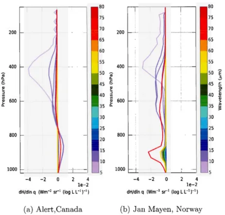
Figure 1. 7 shows the J acobians with respect to humidity for both atmospheric
profiles. For both cases, there is also only a few bands that are sensitive to
24 200
-~
""
(
~ ::, V, V, ~ 600 -a. 80 75 70 65 60 55 50 '" a. 45 .c ~ 40 ~ 200 -400 -~ 600 -35 a. 800 800 -1000 ~ - - -~ - ~ - - - ' -4 -2 0 2 4 le-2 dH/dln q (wm-2 sr-1 (log L L-1 i-1 ) (a) Alert,Canada 1000 -~ - - ---"--- - - - ' -4 -2 0 4 le-2 dH/dln q (wm-2 sr-1 (log L L-1 i-1)(b) Jan Mayen, Norway
80 75 70 65 60 55 50 Ê 3 45 .c ë, C 40 % > 35 ~
FIGURE 1.7: Jacobians with respect to humidity. The Jacobian was computed for a configuration of the instrument with 50 equienergetic bands in the 3.3 to 105 µm interval with respect to humidity and humidity profiles at Alert,Canada (left) and Jan Mayen, Norway (right). The colors of the curves give the wavelength
according to the colorbar
Figure 1. 7a shows the signature of the two effects, which are the greenhouse effect and the presence of an inversion layer. The negative peak at 400 hPa is due to the
greenhouse effect of water vapor. Increasing humidity tends to reduce emission of
radiance by masking the lower warmer layers. The positive part, between 1000
and 750 hPa, is due to the inversion. Increasing humidity elevates the effective
emission altitude, where the atmosphere is warmer due to the inversion. On the
25
band 75-80 µm is sensitive to the variation of water vapor at 900 hPa whereas
the other bands show less variation in their sensitivity. Also, figure 1. 7b shows
redundancy in the bands at 900 hPa.
Background error covariance matrix
The matrix B is the background error covariance matrix. Figure 1.8 represents
the B matrix used for temperature and humidity. The units used are K2 and log(L
L -1 ) 2 for temperature and humidity respectively. This last unit was chosen since
ECCC express humidity in this unit for their NWP and in particular for their
B matrices. In this study, the matrices B are kept constant. The B matrices are
the stationary components of the background term in the ECCC system (Bueh
-ner et al., 2015). Since only the components Brr and Bss of the B matrix are
considered, the calculations for the DFS and analysis error for temperature and
humidity can be made separately. ( a) Temperature 1.5 ~ 1.2
i
0.9 ·; 0.6 ~ 5 0.3 § e 0.0 ~ "' -0.3 800 600 400 200Pressure (hPa)
(b) Humidity 0 0.20 0.18 0.16~ --' 0.14 ~ C 0.12 -~ > 0 0.10 u ~ 0 0.08 t ~ " 0.06 § e 0.04 { 0.02 cc 0.00
FIGURE 1.8: Background error covariances matrices B for temperature (left) and
26
Observation error covariance matrix
The matrix Ris the observation error covariance matrix. Normally, the matrix R
takes into consideration the measurement error, the forward- model error, the
re-presentativeness error, the quality control error, etc (Bormann et al., 2010) but for
this study, only the measurement error was considered. This approximation was
taken according to the conclusions of Bormann et al. (2010) on a physically-based
matrix R for the satellite instruments AIRS and IASI. They show that, in the
thermal IR region, the main contribution to the observation error is the
measure-ment error and also, the interchannel observation error is small (Garand et al.,
2007). Therefore, the matrix R is assumed to be diagonal with the NER values
on the diagonal. The value of NER taken for the IR radiometer is 0.01 wm-2sc1
taken from (Libois, 2016). The range of NER for the instrument AIRS was
ta-ken from the AIRS website (https ://airs.jpl.nasa.gov /index.html) LlB data. The
NER for the synthetic instrument is assumed to be constant for each configuration
and each band. This can be assumed since the error cornes from the sensor and its
error is constant and there is no additional error from the variation in the amount of energy the instrument receives.
The matrix R could be expressed in radiance or in brightness temperature. In
most studies, brightness temperature is used. However, for reasons that will be explained later, the choice was made to express the matrix R in radiance. The
error is expressed in NER or NETD, noise-equivalent temperature difference, if the measure is in radiance or brightness temperature, respectively. The relation
NETD= NER !:::,.).. [jp
oT
27 (1.11) [jpwhere !:::,.>. is the bandwidth and
o
T
is the partial derivative of Planck's emis-sion fonction with respect to temperature. This shows that for a constant NER,
NETD will vary as a fonction of temperature and the spectral width of the band.
To forther illustrate this point, figure 1.9 shows the NETD for a constant NER of
0.01 wm-2sr-1 for an instrument with 10, 15, 20, 25 and 40 equienergetic bands.
The vertical lines represent the widths of the equienergetic bands. The NETD is
not constant for the bands of a configuration. This means that each band has not the same weight when assimilated since its error in brightness temperature is not equal. This allows to see the spectral widths for different configurations of equie
-nergetic bands, which have larger bands at the two extremes of the spectrum. This
figure allows also to compare this experiment with other studies using NETD. It
shows that the NETD, for a configuration with 10 bands, is comparable to the
NETD of AIRS, below 0.5 K (Garand et al., 2007), and of MODIS, less than 0.2
K (King et al., 2003).
NER was chosen in order to work at the sensor level, since it is an extensive qu an-tity. Also, NER remains constant independently of the instrument configuration,
thus when the number of bands increases, the signal-to-noise ratio decreases as
the energy per band decreases. NETD is dependent of the temperature of the
scene and a constant temperature is normally chosen which is not representative
of all situations since temperature is not constant and the bands are not sensitive
28 V) "U C ro ..0 u 25 ·.;::; QJ 00 ~ C ~ 20 0-QJ 4 -0 ~ 15 ..0 E :, z 10 MIR FIR 5 6 8 10 12 15 20 25 30 50 80 105 Wavelength (p.m) 0.5
04
z m -, 0.3 o 0.2 0.1FIGURE 1.9: NETD for différent configurations of equienergetic bands for a black-body at 250 K with a constant NER of 0.01 wm-2sr-1
Comparison of error covariances
0.16 '..._ 0.14 "' '"' 0.12 1 E 0.10 ~0.08 Q) ~ 0.06
'6
0.04 ~ 0.02o
.
o~
!;:::~~~e=::=::;
2
;:=;=
0
==
2
;:;;
s
==
3
;:;;
0
=="=
3
;;
5
::::=
4
=;::
0
~~
45
~=:E
so
Number of bandsFIGURE 1.10: Square root of NER and HBHT for two bands as a fonction of the number of bands of the instrument
Figure 1.10 shows the square root of HBHT with respect to humidity for the
first and last band of the IR radiometer and the square root of R as a fonction
of the number of bands the instrument has. HBHT represents the matrix B in
29
figure shows that B and R have the same magnitude for the band in the interval 75-80 µm. Also, HBHT for the band in the interval 75-80 µm, represented by the
blue line, decreases as the number of bands increases since the quantity of energy
decreases. For the band in the interval 5-10 µm, it increases as the quantity of
energy in the band decreases. This can be explained with figure 1.5 showing that there is a large variation in the transmittance for a small variation in wavelength in the vicinity of 3.3 µm. By taking a larger band, this variation in the transmittance
is lost. In another experiment, by extending the number of bands up to 500 bands,
the value of HBHT decreases drastically at around 200 bands for the first band. With equation 1.4, for the case of the first band, HBHT is much larger than R. This means that the observation is very precise, hence the observation has a lot of weight in the assimilation. For the last band, as HBHT gets smaller compared
to R, the importance of the observation decreases.
1.3 Optimal configuration
With the arrival of spaceborne instruments such as TOVS and AIRS with tho
u-sands of measurements per hour, a method to select subsets of measurements has
been deemed useful (Rodgers, 1998). The DFS has been used to optimally select
bands for the instruments AIRS (Fourrié
&
Thépaut, 2003) and IASI (Rabier et al., 2002) for example.Introduced in section 1.2.1, the DFS is defined as
DFS
=
tr(HK) (1.12)It is an evaluation technique based on the relative errors between the observations
and the prior information (Purser
&
Huang, 1993). It has also been used to quan3
0
of measurements and also on top of measurements already assimilated (McNally
et al., 2006; Lupu et al., 2011)
In this section, the DFS is used to find an optimal configuration for the IR ra-diometer. For each configuration of the IR radiometer, a selection of bands was made sequentially. The first band that maximizes the DFS is selected. The next band selected is the one that, when added to the previous one, adds the largest information content. This process is done until all the bands are selected. Each new band added thus optimally increases the DFS.
Figure 1.11 shows an example of the selection of bands that optimize the DFS with respect to humidity for a configuration of 18 bands. The gray bar represent 95
%
of total information. So, the DFS increases rnpidly for the first 5 bands as -similated and then the gain in assimilating the remaining bands is minimal. Also, 95%
of the total information is obtained when 2 bands are assimilated.1.25 1.20 1.15 vi 1.10
o
1.05 1.00 0.95 0.90 0.85 ' - - ~ - - - _ J 1 2 3 4 5 6 7 8 9 10 11 12 13 14 15 16 17 18Number of bands selected
FIGURE 1.11: DFS for humidity as a fonction of the number of bands selected for an instrument configuration of 18 bands
31
bands, were considered in which the number of bands were increased, each having
the same amount of energy. This process of selecting bands was clone for each
configuration. It is then possible to compare each configuration to get an optimal
configuration for the IR radiometer with respect to temperature and humidity
separately. The observation error covariance matrix is the same for each config
u-ration since it is expressed in terms of NER. This whole process was clone for the
48 atmospheric profiles individually, shown in figure 1.3, and the DFS maps were
then averaged. By doing the calculations for 48 atmospheric profiles, it allows to
see the added value on average and also its variability for the different possible
atmospheric situations in the Arctic.
1.3.1 Number of bands
50 45
Number of selected bands
0 5 10 15 20 25 30 35 40 45 50 ~40ac--1--+--+---l----+---+---"+.LO< "Cl ~ 35 ..0 b30J--,,_ ... ..., w25 . . .._ ... ...-' ..0 E 20 ~ ....... .J,,i' 15 10 5
(a) Temperature
Number of selected bands
0 5 10 15 20 25 30 35 40 45 50 1. 50 raaiiiiiiiiiiliiiiiiiiiiiliiiiiiiiiiliiiiiiiiiiliiiiiiiiiiiiiiiiiiiiiiiiiiiiiiiiiiilii-1 45 1. ~40~ +--+--+---1---+----1---+--'
1
.
-g
ro35 ___ ,__.,___--1--+--+---1----' l. ~ 30 -.Cl--.1---1-...J.._-L--I 0 1. w 25 ..0o
.
§
20 z ~ ...o
.
15o
.
10 5 (b) Humidity 1.80 1.65 1.50 1.35 V1 1.20 ~ 1.05 0.90 0.75 0.60FIGURE 1.12: Averaged DFS maps where the x-axis is the number of bands of the
instrument and the y-axis is the number of bands selected. The color correspond
to the DFS associated to a combination of number of bands of the intrument and
- - - - -- - - --~--- - - - -- - - -- -- - - -- - - -- - - -- - -
-32
Figure 1.12 shows the DFS of different configurations with respect to temperature and humidity for a synthetic IR radiometer with a NER of 0.01 wm-2sr-1 and
a spectral range of 3.3 µm to 105 µm. The ordinate axis represents the number of equienergetic bands of the instrument whereas the abscissa axis represents the subset of bands selected. The total number of bands varies between 5 to 50 bands. Figure 1.11 shows a line of figure 1.12b for the configuration with 18 bands. The color of the case represents the value of the DFS for this configuration. The co -lorbars of figure 1.12 are not the same since the DFS maximal is different for temperature and humidity. The diagonal represents the cases when all the bands are assimilated for each configuration. This shows that having more bands is not always the best configuration, since the DFS is not increasing as the number of bands increa. ·es. This will be further discussed in the next section to cxplain why that is.
Those maps show that sometimes increasing the number of bands by one can re -duce the DFS by a larg amount. For example, by splitting the spectrum in 13 bands instead of 12 reduces the total DFS from 1.4384 to 0.9979 for humidity. This is due to the micro-windows in the transmittance of water vapor and the positions of the bands. Depending of the beggining and the end of a specific band,
for example the sixth band for configurations of 12 and 13 bands, there can be a large variation in the averaged transmittance. This can be also viewed with the Jacobians. Figure 1.13 shows the Jacobians for those two cases. Figures 1.13a and 1.13b show the Jacobians with respect to temperature for the cases with 12 and 13 bands. For 13 bands, the peak of the band in the interval 5-10 µm decreases by a factor of 2. 79. The band in the interval 75-80 µm is almost constant even if the band is narrower. The bottom panels of figure 1.13 show the Jacobians with respect to humidity for the same cases. The conclusions for the Jacobians with
33
respect to humidity are the same as for the Jacobians with respect to temperature.
This shows that not only the number of bands is important but also the position of those bands. 80 80 75 75 200 70 200 70 65 65 60 60 55 55 400 400 50 50 45 45 40 40 600 600 35 35 30 30 25 25 800 800 20 20 15 15 10 10 1000 1000 0 1 2 3 4 5 6 7 0 1 2 3 4 5 6 7 dH/dT (wm-i 5,-1 K-1 )le-3 dH/dT (Wm-2 sr-1 K-1 )le-3 (a) 12 bands (b) 13 bands 80 1 1 1 80 75 75 200 70 200 70 65 65 60 60 55 55 400 400 50 50 45 45 40 40 600 600 35 35 30 30 25 25 800 800 20 20 15 1 15 10 10 1000 1000 1 1 1 -4 -2 4 -4 -2 0 4 1e-2 le-2 dH/dln q (wm-2 sr-1 (log L L-11-1) dH/dln q (Wm-2 sr-1 {log L L-11-1) (c) 12 bands (d) 13 bands
FIGURE 1.13: Jacobians for atmospheric profile at Alert, Canada. The first row shows the Jacobians with respect to temperature and the second row with respect
34
Figure 1.12a shows the DFS map with respect to temperature. The optimal confi -guration of the averaged map is 50 bands. The maximal DFS is 1.686 for this configuration. For the different atmospheric cases, 32 out of the 48 cases, the configuration with 50 bands is the optimal configuration and the maximal DFS
varies between 1.047 and 2.433. For the optimal configuration of 50 bands, 95%
of the information is contained by taking a subset of 4 bands.
Figure 1.12b shows the DFS with respect to humidity. The optimal configuration
of the averaged map is 50 bands, with a DFS maximal of 1.883. For the
indivi-dual maps, the optimal configuration is, 43 out of 48, the configuration with 50 bands. For the different atmospheric cases, the maximal DFS varies between 0.981
and 2.709. For the optimal configuration of 50 bands, 95% of the information is
contained by taking a subset of 3 bands.
Thus, the configuration for the IR radiometer taken for the remaining work is with
50 bands for both temperature and humidity, which will be called the optimized
IR radiometer. The following discussion consider other configurations but are not
used in the next section.
Another interesting way to analyze those maps is by having a constraint on the number of bands an instrument can have. A radiometer is operated with a filt
er-wheel, thus as the number of bands increases, the rate of repetition decreases
and also the cost increases, thus a constraint on the number of bands is needed.
By taking the vertical line which corresponds to the constraint on the number of
bands M, it gives the optimal subset of bands M, if M is larger than the total
35
have 10 bands, the optimal configuration with respect to humidity is not to split
the spectrum in 10 equienergetic bands (DFS of O. 7626) but to take a subset of
10 bands of the spectrum splitted in 50 bands (DFS of 1.8718).
It
shows that itis better to take thinner less energetic bands since those bands are better located
with respect to the transmittance of water vapor. This was explained previously
with the example with 12 and 13 bands.
VI
"
0 500 450 400 350 ~ 300 .c ~ 250 (1) .c § 200 z 100 50Number of selected bands
50 100 150 200 250 300 350 400 450 500
0.8
0.7
0.6
0.5
FlGURE 1.14: DFS map for humidity for up to 500 equienergetic bands in steps
of 10 bands for the selected profile at Alert, Canada
Figure 1.14 shows a DFS map for humidity up to 500 bands in steps of 10 bands
for the profile shown in figure 1.4a. The optimal configuration is 150 bands. Up
to 200 bands, the DFS is around 0.6 to 0.8 whereas from 200 bands up to 500
bands, the DFS saturates to around 0.15. This shows that hyperspectral bands
for a radiometer have no value with the instrument resolution of 0.01 wm-2sr-1
36
1.3.2 Order of the wavelengths
Number of selected bands Number of selected bands 0 5 10 15 20 25 30 35 40 45 50 0 5 10 15 20 25 30 35 40 45 50 50 50 80 75 45 45 70 VI 40 VI 40 65 60 ~ "Cl "Cl 55 [ ~ 35 ~ 35 ..0 ..0 50 ~ 'ci 30 'ci 30 45 ai J.... J.... 40 ~ QJ 25 QJ 25 ..0 ..0 35 aï E 20 E 20 30 ~ :J :J z z 25 ~ 15 15 20 10 10 15 10 5 5 5 (a) Ternperature (b) Hurnidity
FIGURE 1.15: Wavelengths of the bands selected over the 48 atmospheric profiles
The previous section seeked to find the number of bands needed to optimize the
IR radiometer. In this section, the wavelengths of those bands most often selected
over the 48 atmospheric profiles are described and analysed. Figure 1.15 shows the
wavelengths in microns of the bands most often selected for the 48 atmospheric
profiles for temperature and humidity in the same order as for the maps in figure
1.12. The different wavelengths are shown by intervals of 5 µm.
For temperature, figure 1.15a, the first band selected is the band in the FIR region
70-75 µm and the second band is in the interval 5-10 µm. This is for configur
a-tions up to 13 bands. For the configurations with 9 and 14 bands, around half the