AND
ASTROPHYSICS
Three photometric methods tested on ground-based data
of Q 2237+0305
?
I. Burud1,2, R. Stabell2,3, P. Magain1,??, F. Courbin1,4, R. Østensen1,5, S. Refsdal3,6, M. Remy1, and J. Teuber3
1
Institut d’Astrophysique, Universit´e de Li`ege, Avenue de Cointe 5, B-4000 Li`ege, Belgium
2
Institute of Theoretical Astrophysics, University of Oslo, Pb. 1029 Blindern, N-0315 Oslo, Norway
3
Centre for Advanced Study, Drammensveien 78, N-0271 Oslo, Norway
4
URA 173 CNRS-DAEC, Observatoire de Paris, F-92195 Meudon Principal C´edex, France
5
Department of Physics, University of Tromsø, N-9037 Tromsø, Norway
6
Hamburger Sternwarte, Gojenbergsweg 112, D-21029 Hamburg, Germany
Received 29 June 1998 / Accepted 24 August 1998
Abstract. The Einstein Cross, Q 2237+0305, has been photo-metrically observed in four bands on two successive nights at NOT (La Palma, Spain) in October 1995. Three independent algorithms have been used to analyse the data: an automatic image decomposition technique, a CLEAN algorithm and the new MCS deconvolution code. The photometric and astrometric results obtained with the three methods are presented. No pho-tometric variations were found in the four quasar images. Com-parison of the photometry from the three techniques shows that both systematic and random errors affect each method. When the seeing is worse than1.000, the errors from the automatic im-age decomposition technique and the Clean algorithm tend to be large (0.04-0.1 magnitudes) while the deconvolution code still gives accurate results (1σ error below 0.04) even for frames with seeing as bad as1.007.
Reddening is observed in the quasar images and is found to be compatible with either extinction from the lensing galaxy or colour dependent microlensing.
The photometric accuracy depends on the light distribution used to model the lensing galaxy. In particular, using a numeri-cal galaxy model, as done with the MCS algorithm, makes the method less seeing dependent. Another advantage of using a numerical model is that eventual non-homogeneous structures in the galaxy can be modeled.
Finally, we propose an observational strategy for a future photometric monitoring of the Einstein Cross.
Key words: quasars: individual: Q 2237+0305 – gravitational lensing – techniques: image processing
Send offprint requests to: I. Burud, Li`ege address,
?
Based on observations obtained at NOT, La Palma.
??
Maˆıtre de Recherches au Fonds National Belge de la Recherche Scientifique
1. Introduction
The gravitational lens system Q 2237+0305, known as the Ein-stein Cross, is one of the most promising objects to observe intensity variations due to microlensing of quasar images. The object, discovered by Huchra et al. (1985), consists of four im-ages of the same quasar at z = 1.69 lensed by a foreground spiral galaxy atz = 0.04. The maximum angular separation of the components is about1.008. Due to the proximity of the lens and the high degree of symmetry of the system, the time delays between the images are of the order of one day. Intrinsic varia-tions of the source therefore show up almost simultaneously in all four quasar images, hence making them easy to distinguish from microlensing effects. This system with a low-redshift lens is an ideal case for studying microlensing effects, since the light paths to the different QSO images pass through the bulge of the galaxy, hence increasing the probability of gravitational influ-ence by single stars (Chang & Refsdal 1979, Paczynski 1986, Kayser et al. 1986, Kayser & Refsdal 1989). In addition we note that the angular size of the Einstein ring for a given lens mass is larger than for systems with higher lens redshifts.
However, detecting faint intensity variations in multiply imaged QSOs requires very accurate photometry. For most gravitationally lensed QSOs, this is not a straightforward task, Q 2237+0305 being one of the most complicated cases. Given the blending of the QSO images, aperture photometry is ex-cluded and profile fitting photometry is not trivial. Moreover, since the foreground galaxy has a sharp nucleus creating a non-uniform and fast-varying background, the light distribution of the lensing galaxy has to be modeled carefully.
Several methods and algorithms have been developed to perform PSF photometry of blended sources and more spe-cific codes have been developed to treat the Einstein Cross. We compare in the following, three of these methods (described in Sect. 3): an automatic PSF fitting technique (M. Remy 1996, hereafter the Fitting method), an interactive CLEAN algorithm (R. Østensen 1994), and a deconvolution method (P. Magain, F. Courbin & S. Sohy 1998, hereafter MCS).
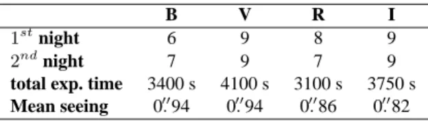
Table 1. Log of observations of the Einstein Cross from the 10thand
11thof October 1995. The first two lines show the total number of
frames in each band. The next two lines give the total exposure time and the mean seeing value.
B V R I
1stnight 6 9 8 9
2ndnight 7 9 7 9
total exp. time 3400 s 4100 s 3100 s 3750 s
Mean seeing 0.0094 0.0094 0.0086 0.0082
For this purpose, numerous images of the Einstein Cross were taken on two successive nights at the Nordic Optical Tele-scope (NOT) at La Palma, Canary Islands (Spain). A homo-geneous set of data taken over a short time scale with a good temporal sampling was obtained. No physical intensity varia-tions were likely to be detected in the object during such a short period so that the data set is very well suited for performing photometric tests. For each method, we measured the photo-metric robustness with respect to the seeing variations in optical B, V, R, I-bands.
If we detected real variations during the two nights, we would have had the chance to observe either a high amplifi-cation microlensing event (if the variation had occurred in one image only) or an intrinsic fluctuation in the quasar itself, which could have led to the determination of the time delay for this system.
2. Observations
The observations took place at the NOT on the nights of October 10 and 11, 1995. We used the CCD camera BroCam 1 equipped with a thinned backside illuminated TEK 1024 CCD with a conversion factor of q = 1.7e−ADU−1, a readout noise of 6.5e−and a pixel size of0.00176. Sequences of exposures were obtained through the filtersB, V, R and I (in this order). The total number of frames obtained of the Einstein Cross in each band, as well as the total exposure time and the mean seeing value are summarized in Table 1. The seeing of the frames varied between0.006 and 1.007.
Bias subtraction, flat-field correction (sky-flats) and cosmic ray removal were applied to the raw data using the ESO MIDAS routines. In order to model and subtract low frequency sky vari-ations across the frames, bi-quadratic polynomial surfaces were fitted to a well sampled grid of empty regions in each individual frame.
3. Photometric methods
3.1. The fitting method
A profile fitting method has been developed in the MIDAS environment by M. Remy (1996) in order to obtain accurate photometric measurements of multiply imaged quasars. This method has already been applied to other lensed systems, (e.g.,
H1413+117, the Cloverleaf, Østensen et al. 1997). Unlike the Einstein Cross, the Cloverleaf system does not suffer from the contamination of a bright and complicated foreground lens, and is therefore much easier to study.
In the present case, the magnitudes of the quasar images were determined by fitting simultaneously numerical PSFs to the point sources, and a de Vaucouleurs function (R−1/4) to the galaxy. An additional Moffat profile was also fitted (still simultaneously) in order to model the point-like galaxy nucleus. All the parameters were adjusted by the program, using aχ2 minimization. The intensity and positions for the four numerical PSFs and for the Moffat profile were determined as well as the shape and rotational parameters of the Moffat and the de Vaucouleurs model.
The technique was tested in different ways on our images. First, the fit was performed with all the parameters free on the whole data set. From these results, we calculated the mean po-sitions of the QSO components and the galaxy nucleus. Then we ran the program with the position parameters fixed relative to component A. Furthermore, a galaxy model with fixed shape parameters was obtained by extracting the galaxy from the best result in each band. It was then convolved to the respective see-ing of each individual frame. Another fit was performed with a fixed galaxy model centered on the nucleus, i.e. only its inten-sity was left as free parameter. The advantage of freezing the relative positions of the QSO images and the galaxy model is to minimize the number of free parameters in the fit. On the other hand, if the positions and the galaxy model are not accurate, we may introduce systematic errors. In the present case, the best χ2
fit was obtained with all the positions fixed relative to com-ponent A, and a de Vaucouleurs profile with fixed parameters. Sect. 4.1 presents the results obtained in this way.
3.2. A CLEAN algorithm
A program for CLEAN photometry of overlapping point sources has been developed by R. Østensen (1994), and implemented us-ing IDL. This program, called XECClean, has been specifically designed to perform photometry on the Einstein Cross and has been applied to the NOT monitoring data of the object (Østensen et al. 1996). As for the Fitting method, the programme has also been used on the monitoring data of H1413+117 (Østensen et al. 1997).
XECClean applies a semi-analytical PSF-profile fitting pro-cedure adapted from the DAOPHOT package (Stetson 1987), and “deconvolves” the images using an interactive CLEAN al-gorithm (e.g., Teuber 1993). A PSF is successively fitted and removed from each QSO image until a first convergence of the parameters is reached. Once the point sources are removed, a de Vaucouleurs profile with fixed shape parameters is centered on the galaxy nucleus and convolved to the seeing of each frame. This model is fitted to the lensing galaxy and subtracted from the image. Then the quasar components and the galaxy are it-eratively restored, fitted again, and removed until convergence is reached. This is repeated as many times as necessary for ob-taining satisfactory residuals for each frame.
3.3. The MCS deconvolution algorithm
A new deconvolution method has been developed by Magain et al. (1998). Contrary to traditional methods of deconvolution, this algorithm allows not only a significant increase in the spatial resolution of the images, but also to perform accurate photomet-ric and astrometphotomet-ric measurements on the deconvolved frames.
The algorithm is based on the principle that sampled data cannot be fully deconvolved without recovering Fourier fre-quencies higher than the Nyquist frequency, and violate the sampling theorem. A sampled image should therefore not be deconvolved by the total PSF but by a narrower function chosen so that the resolution of the deconvolved image is compatible with the adopted sampling.
The image is decomposed into a sum of point sources plus a diffuse background. The background is constrained to be smoothed on the length scale of the final resolution, chosen by the user. The best model image is computed by minimizing the χ2
using a modified version of the conjugate gradient method (Press et al. 1989 ). Positions and intensities of the point sources as well as the image of the deconvolved background are given as output of the deconvolution procedure.
Successful results have already been obtained on several gravitational lens systems (e.g., Courbin et al. 1998a, 1998b). In the present case, we chose the pixel size of the deconvolved frame to be half the one in the original data,0.00176/2 = 0.00088. Furthermore, we adopted for the deconvolved point source a Gaussian profile with a FWHM of 3 (small) pixels, which al-lows us to reach a final resolution of0.0026. The deconvolution of our images was performed in two steps. First, the frames in a given filter were averaged, giving a deep image of the object. This image was deconvolved in order to obtain an accurate nu-merical model of the lensing galaxy. Since the galaxy profile varies sharply in the vicinity of the nucleus, we applied a vari-able smoothing parameterλ across the field, in order to avoid local over- or underfitting of the data (see Magain et al. 1998). Since the nucleus-shape is close to that of a point source, but not exactly, we added a quasi-point-source described by a Moffat profile, for the nucleus. Its intensity, position and shape param-eters were all determined by the deconvolution program.
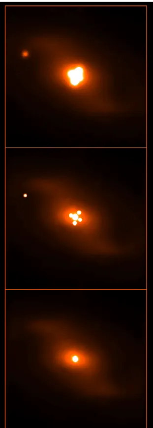
Fig. 1 presents the result obtained from the stack of our R-band frames. The top and the middle panels show the observed and the deconvolved frame respectively, and the bottom panel displays the numerical galaxy model obtained by the algorithm. Both the point sources (quasar components and foreground star) and the lensing galaxy appear clearly without any deconvo-lution artifacts. The separation of the point sources from the background allows one to study the deflector alone, without the disturbing light from the quasar’s images. We could in this way determine an accurate numerical model for the lensing galaxy, that can be used for future photometric monitoring.
After a numerical model of the galaxy had been obtained in each band, it was used as a fixed background for the deconvolu-tion of the individual frames. Only a multiplicative factor and an additive term were applied in order to correct for different ex-posure times (e.g., shutter effects) and varying sky-levels. The
Fig. 1. [Top]: Stack of 12 R band frames with a seeing of ∼0.008. [Mid-dle]: Deconvolved frame using the MCS algorithm. The resolution is
now 0.0026. [Bottom]: Deconvolved numerical galaxy model. All the
Table 2. B-band photometric results: mean magnitude and standard
deviations
Fitting Clean Deconv
A 17.612 ± 0.025 17.626 ± 0.033 17.655 ± 0.029 σmean ±0.007 ±0.009 ±0.008 B 17.754 ± 0.040 17.741 ± 0.030 17.754 ± 0.023 σmean ±0.011 ±0.008 ±0.006 C 18.937 ± 0.076 18.881 ± 0.073 18.885 ± 0.040 σmean ±0.021 ±0.020 ±0.011 D 19.155 ± 0.034 19.111 ± 0.121 19.220 ± 0.040 σmean ±0.009 ±0.033 0.011
Table 3. V-band photometric results: mean magnitude and standard
deviations. We have removed one of the frames with a FWHM=1.0063
in the results from the Fitting and CLEAN algorithms.
Fitting Clean Deconv
A 17.257 ± 0.018 17.278 ± 0.019 17.276 ± 0.016 σmean ±0.004 ±0.004 ±0.004 B 17.414 ± 0.014 17.428 ± 0.022 17.425 ± 0.015 σmean ±0.003 ±0.009 ±0.004 C 18.531 ± 0.062 18.389 ± 0.028 18.415 ± 0.035 σmean ±0.015 ±0.009 ±0.008 D 18.801 ± 0.070 18.734 ± 0.075 18.704 ± 0.031 σmean ±0.017 ±0.022 ±0.007
frames were deconvolved both separately and simultaneously. The advantage of simultaneous deconvolution is that the solu-tion is compatible with all the images considered. The intensities of the point sources are allowed to converge to different values from one frame to another so that intrinsic variations in the ob-ject can be detected, while the positions of the point sources are constrained by all the images used.
4. Results
4.1. Photometric results
Our photometric magnitudes are calibrated by means of Yee’s (1988) reference star, using the transformation equations and revised values given by Corrigan et al. (1991). No significant intensity variation was detected on the data during the two nights of observation. Therefore a mean magnitude could be calculated for each QSO image and a1σ error for the results obtained with each method. These values, as well as the calculated error on the mean magnitude, are shown in Tables 2, 3, 4, and 5 for theB,V , R, I filters respectively. The standard deviation of the mean σmeanwas calculated in order to give an estimate of the error for each QSO image in each filter and is simply the standard deviation for all the frames divided by the square root of the number of frames used.
In order to make sure that the magnitudes of the QSO images did not vary during the run, we looked for possible systematic correlations between the results of the different methods. No such correlation was found. Therefore we can safely assume
Table 4. R-band photometric results: mean magnitude and standard
deviations. We have removed one of the frames with a FWHM=1.0048
in the result from the Fitting technique.
Fitting Clean Deconv
A 17.078 ± 0.020 17.093 ± 0.014 17.106 ± 0.021 σmean ±0.006 ±0.004 ±0.005 B 17.262 ± 0.027 17.274 ± 0.014 17.291 ± 0.023 σmean ±0.008 ±0.004 ±0.006 C 18.227 ± 0.030 18.109 ± 0.032 18.093 ± 0.042 σmean ±0.009 ±0.008 ±0.011 D 18.522 ± 0.048 18.441 ± 0.039 18.378 ± 0.032 σmean ±0.014 ±0.010 ±0.009
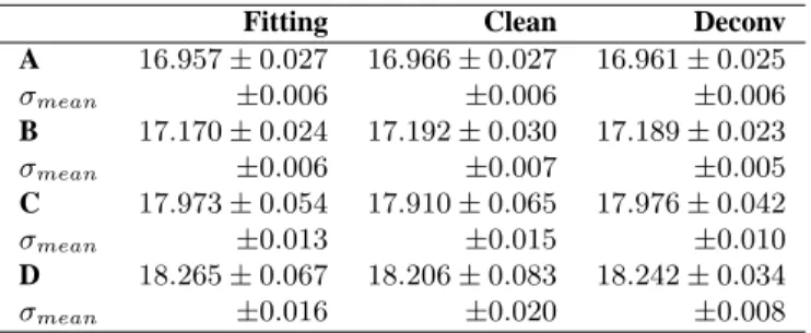
Table 5. I-band photometric results: mean magnitude and standard
deviations
Fitting Clean Deconv
A 16.957 ± 0.027 16.966 ± 0.027 16.961 ± 0.025 σmean ±0.006 ±0.006 ±0.006 B 17.170 ± 0.024 17.192 ± 0.030 17.189 ± 0.023 σmean ±0.006 ±0.007 ±0.005 C 17.973 ± 0.054 17.910 ± 0.065 17.976 ± 0.042 σmean ±0.013 ±0.015 ±0.010 D 18.265 ± 0.067 18.206 ± 0.083 18.242 ± 0.034 σmean ±0.016 ±0.020 ±0.008
that the QSO images did not vary and we can use the data set to compare the three algorithms.
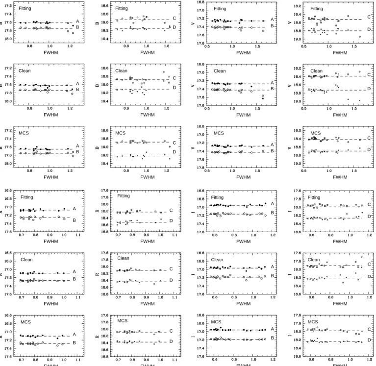
For the Fitting method and the CLEAN algorithm, the pho-tometry depends on the seeing of the frame, i.e., the errors in-crease when the seeing gets worse. One frame in theR-band and one in theV -band were removed from the analysis using these two methods, since they would have biased the results. We find that only the frames with a seeing better than1.001 allow us to obtain a photometric accuracy better than 0.05 magnitudes with these two methods. The MCS algorithm is less dependent on seeing and all the frames with a seeing up to1.007 gave photo-metric errors below 0.04 magnitudes. If we consider data with an integrated S/N ∼ 700 over one point source and a see-ingF W HM ≤ 1.0000, the overall 1σ error bar is below 0.02 magnitudes for the A and B components and below 0.04 magni-tudes for the C and D components, for all three methods. Fig. 2 presents the magnitudes for the B, V , R and I band frames respectively, measured with the three different techniques. The magnitudes are plotted as a function of seeing (in arcseconds). One of the frames with a seeing of ∼ 1.0048 was discarded from theR-band figures. We notice systematic differences of the or-der of 0.1 magnitudes between the three methods for the C and D components in theR-band. This is more than the standard devia-tions calculated on the mean values and indicates that systematic errors introduced by the analysis algorithm might significantly affect the photometry of the Einstein Cross. In several cases, a correlation between the four QSO images is observed in the frames with bad seeing values. This may be due to inaccurate scaling of the galaxy.
C D Fitting FWHM A B Fitting FWHM A B Clean FWHM C D Clean FWHM A B MCS FWHM C D MCS FWHM C D Fitting FWHM A B Fitting FWHM A B Clean FWHM C D Clean FWHM A B MCS FWHM C D MCS FWHM C D Fitting FWHM A B Fitting FWHM A B Clean FWHM C D Clean FWHM A B MCS FWHM C D MCS FWHM C D Fitting FWHM A B Fitting FWHM A B Clean FWHM C D Clean FWHM A B MCS FWHM C D MCS FWHM
Fig. 2. Photometric magnitudes as a function of seeing (in arcseconds) for the B, V , R and I frames. Note that in the V -band, the magnitude
of component D, derived with the Fitting method on the image with a seeing of 1.0063 is outside the plot.
The results displayed in Fig. 2 have motivated photometric tests on simulated frames of the object, in order to investigate the effects of random and systematic errors on the photometry. Syn-thetic images were created with the three different models of the lensing galaxy (de Vaucouleurs profiles and numerical models) and with different seeing values. We found that the photomet-ric results from the Fitting method and the CLEAN algorithm depend on both seeing and galaxy model. Implementing an ac-curate numerical galaxy model into the Fitting and the Clean algorithms would therefore certainly improve their efficiency
and accuracy, in particular for bad seeing values. The random errors are of the same order as the statistical errors we calcu-lated from the real frames. The systematic errors are smaller than 0.05 magnitudes for the A and B component, but up to 0.1 magnitude for the C and D components both for the Fitting method and the CLEAN algorithm when tested on the images created with different galaxy models. No systematic correlation was found between the photometry of images with different galaxy models analysed with different methods, indicating that these systematic errors are difficult to correct for.
-0.95 -0.90 -0.85 -0.80 -0.75 0.60 0.55 0.50 0.45 -0.75 -0.70 -0.65 -0.60 1.75 1.70 1.65 1.60 0.50 0.55 0.60 0.65 0.70 1.30 1.25 1.20 1.15 1.10 -0.20 -0.15 -0.10 -0.05 0.00 1.00 0.95 0.90 0.85
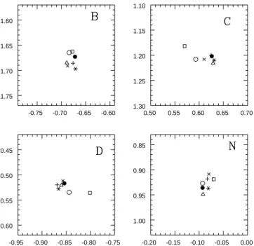
Fig. 3. Mean positions relative to the A component from all methods.
The x and y axis give respectively R.A. and Declination in arcseconds relative to A. The symbols correspond to the following: × Fitting, 2 CLEAN, 4 MCS, • Crane et al. , + Rix et al., ◦ Østensen et al., ∗ Blanton et al.
For the deconvolution method, the systematic errors are smaller than 0.05 magnitude for all the components, and the results depend much less on the seeing of the frames since a detailed numerical galaxy model is used.
4.2. Astrometric results
The relative positions measured for the four components using the different methods are in fairly good agreement, not only with one another, but also with the positions determined from obser-vations with the HST (Crane et al. 1991, Rix et al. 1992 and Blanton et al. 1998) and the results from the photometric mon-itoring published by Østensen et al. (1996). Fig. 3 presents the geometry of the object relative to component A, as derived from the three methods, and compared with previously published as-trometry. Note that only the frames with a sub-arcsecond seeing were used for the Fitting method and the CLEAN algorithm. We found that the astrometric accuracy of these two methods sig-nificantly decreases with bad seeing. With a seeing worse than 1.001, typical errors of 0.0002 are observed. The errors seem to be random with the Fitting method, whereas with the CLEAN algorithm, the positions measured for the C and D component tend to drift towards the galaxy’s nucleus when the seeing gets worse.
The astrometry obtained with the deconvolution algorithm is much less seeing dependent as soon as an accurate numerical galaxy model is used. However, obtaining such a galaxy model requires the nucleus’ position to be well estimated from high S/N data (see Sect. 3.3). This is particularly true in theB-band
Fig. 4. Contour plots of the numerical galaxy model from the MCS
deconvolution code in the I band. Both axis are in arcseconds. North is up and East is to the left.
where the nucleus is very faint and its position less accurate (about0.0005).
5. The lensing galaxy
5.1. Morphology
As described in Sect. 3.3 and shown in Fig. 1, the MCS code produces a deconvolved numerical galaxy both with and with-out nucleus. The contour plot displayed in Fig. 4 clearly reveals a bar in the central 10 arcseconds of the galaxy. It has a very similar shape in theV and R bands whereas in the B band the S/N of the data is too low to derive an accurate galaxy profile. The bar cannot be correctly modeled by a pure analytical pro-file, even in the centre of the galaxy, as in fact suggested by the significant residuals obtained with the Fitting and the Clean al-gorithms. Photometry obtained by using only analytical models is therefore likely to be biased.
5.2. Extinction
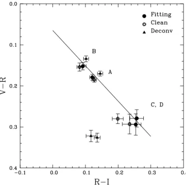
From our analysis, we found that the A component is reddened relative to B, and that the C and D components are both red-dened relative to A. Fig. 5 shows theV − R colour as a function ofR − I. The error-bars indicated are the errors on the mean (σmeanin Tables 2-5). If the reddening is due to extinction from the galaxy, the four quasar images should lie approximately on a straight line representing the extinction law for the lens galaxy. Since it has been suggested that this law is similar to the one of our Galaxy (Yee 1988), the mean extinction law for the latter is shown on Fig. 5, as a solid line with a slope of 0.86 (Vakulik et al. 1997). Cardelli et al. (1989) showed that in theV -R-I domain, the shape of the extinction law is insensitive to the parameter RV = AV/E(B-V), thus independent on the origin of the ex-tinction (e.g., interstellar matter, dense clouds). From Fig. 5, the results from the Fitting and the CLEAN as well as the A and B magnitude from MCS could be interpreted as extinction. The positions of components C and D compared to A and B on the
Fig. 5. V-R as function of R-I for the three different methods with
error-bars on the mean of all the frames (σmeanin Tables 2-5). The mean
extinction law for our Galaxy is drawn as a solid line through the mean colour of the A component. See Sect. 5 for an explanation of the C and D points.
straight line can be explained by reddening due to the tilt of the galaxy in the direction of C and D. This tilt might even explain the reddening of A compared to B. However, we point out that the magnitudes obtained with Fitting and CLEAN in the differ-ent bands do not agree with each other, but by coincidence the differences cancel out in this particular colour plot.
Considering the differences in C and D between the three methods we can not confirm the presence of a mean extinction law. In particular, the C and D results from MCS could be in-terpreted as a long time colour dependent microlensing effect. When the source passes a microcaustic, its inner and hence bluer parts may be more amplified than the outer emission line region of the accretion disk. (Kayser et al. 1986 and Wambsganss & Paczy`nski, 1990 ). This is even true for sources angularly larger than the Einstein radius of the lens (Refsdal & Stabell 1991).
We found a colour excess of B with respect to A of∆E(V − I) = −0.08 ± 0.02, magnitudes. This is in agreement with Vakulik et al. (1997) who found∆E(V − I) = −0.12 ± 0.05 magnitudes, also from observations taken in 1995. However, Yee et al. (1988) found that B was reddened relative to A,E(g − i) = +0.08 ± 0.03.
A possible change in the relative colours over time might be explained by colour dependent microlensing or, less likely, by dust extinction that varies over time (e.g., Rix et al. 1992). The reason for a colour change in the Einstein Cross will remain unclear unless long term multicolour photometric monitoring ( or preferably spectrophotometry) is carried out on a dedicated telescope.
6. Discussion and conclusions
The two most complete light curves from photometric monitor-ing of the Einstein Cross have been published by Corrigan et al. (1991) and more recently by Østensen et al. (1996). Although several obvious microlensing events have been observed, no precise estimates of the photometric errors have been discussed so far. Moreover, better sampling of the light curves, as well as more accurate photometric measurements are needed in order to interpret the observed intensity differences in detail. In the present study, a set of observations in four bands was obtained during two successive nights. Since the time delay for the Ein-stein Cross is of the order of one day, observations on a short time scale would make it possible to separate intrinsic variations from microlensing effects.
A bright star is available on all our frames to perform PSF photometry with the three different methods considered in this paper. The seeing during the two nights was variable (0.006-1.007), which allowed us to quantify the seeing dependence of the dif-ferent methods applied.
Differences are observed between the photometric measure-ments obtained with the three methods (see Fig. 2). All the meth-ods show random errors that, as one should expect, increase with bad seeing. In addition, systematic errors in one or more of the methods are also present, especially for the fainter components of Q 2237+0305. For each QSO component, the dispersion be-tween the mean magnitude obtained with the 3 techniques is larger than the error measured (σmean) for each method. Pho-tometric measurements performed on simulated frames also showed that the systematic errors depend both on the seeing and on the galaxy model used to describe the deflector. The Fitting and the Clean algorithms produce large errors (0.04-0.1 magnitudes) for the two faint quasar components (C and D) when the seeing is worse than1.000. The errors from the MCS algorithm are below 0.04 magnitudes and less dependent on the seeing when a numerical galaxy model is used.
If only subarcsecond seeing frames are considered, we find that all three methods could have detected intensity variations with a minimum amplitude of 0.02 and 0.04 magnitudes in com-ponents A, B and C, D respectively. The latter errors are given for one individual measurement and can be improved by using several frames. When the exposures are of ∼200s, as in our case, about 10 frames can be obtained in one hour of observation. If 10 frames with a subarcsecond seeing are obtained, the ran-dom error will be0.02/√10 = 0.006 and 0.04/√10 = 0.013 magnitudes for A, B and C, D respectively.
Assuming that systematic errors are present, it is reasonable to think that they would be more important when an analyti-cal galaxy model is used, rather than when a purely numerianalyti-cal model is applied. Even if an analytical de Vaucouleurs profile can fit the central bulge of the galaxy, it cannot model the bar in the spiral galaxy, and we cannot exclude that this may affect the photometry of the quasar images. Moreover, a good numerical model obtained from high S/N data can represent high frequency structures in the galaxy which would be neglected by an ana-lytical model. For example, H ii regions in the lens galaxy can
only be modeled by a numerical profile. Such clumpy structures, likely to emit in theHαline, would then make inaccurate the R-band photometry obtained with any analytical galaxy model. In such a case, the photometry of the C and D components would be most affected since their positions are along the bar of the galaxy, where most of the H ii regions should lie. The largest photometric differences between the methods investigated here are indeed present in theR-band, but Hα-imaging would be needed to confirm such an effect by directly imaging the H ii clumps. We should also point out that finding a numerical galaxy involves a larger number of free parameters. In the present case, we cannot rule out the possibility that the S/N in our frames was too low to obtain a unique numerical model.
Based on the published light curves and the present study, we propose the following observational strategy for a future pho-tometric monitoring of the Einstein Cross. The aimed sampling of the points on a light curve should be compared with typical time scales of microlensing events. Since time scales as short as 14 days have been observed (Østensen et al. 1996), a sampling of the order of a few observations per night should be aimed at. Furthermore, since intensity variations of 0.05 magnitudes or less can be expected (Østensen et al. 1996), it is important to ensure a photometric accuracy well below this value. As shown in our study, using several data frames (up to 10 with a 2m class telescope) to derive any individual photometric measurement would yield random error bars smaller than 0.01 magnitude for subarcsecond observing conditions, and would allow such a monitoring program.
However, one cannot expect subarcsecond conditions over observing runs as long as several nights. Given this observa-tional constraint, it is likely that the best photometric accuracy will be obtained by using a detailed numerical galaxy model. We have shown that such a galaxy model can be constructed from high S/N frames with the MCS algorithm and that accurate pho-tometry can be achieved by applying this model in connection with simultaneous deconvolution of all the frames.
Acknowledgements. We wish to thank S. Sohy for help with the MCS
algorithm, and J.P. Swings for support. IB, FC, and RØ are supported in part by contract ARC94/99-178 “Action de Recherche Concert´ee de la Communaut´e Franc¸aise (Belgium)” and Pˆole d’Attraction Interuni-versitaire, P4/05 (SSTC, Belgium).
References
Blanton, M., Turner, E.L., Wambsganss, J., 1998, preprint astro-ph/9805359
Cardelli, J.A., Clayton, G.C., Mathis, J.S., 1989, ApJ, 345, 245 Chang, K., Refsdal, S., 1979, Nature, 282, 561
Corrigan, R.T., Irwin, M.J., Arnaud, J., et al., 1991, AJ, 102, 34 Courbin, F., Lidman, C., Magain, P., 1998a, A&A, 330, 57 Courbin, F., Lidman, C., Frye, B., et al. 1998b, ApJ, 499, L119 Crane, P., Albrecht, R., Barbieri, C., et al. 1991, ApJ, 369, L59 Huchra, J., Gorenstein, M., Kent, S., et al., 1985, AJ, 90, 691 Kayser, R., Refsdal, S., Stabell, R., 1986, A&A, 166, 36 Kayser, R., Refsdal, S., 1989, Nature, 338, 745 Magain, P., Courbin, F., Sohy, S., 1998, ApJ, 494, 472
Østensen, R., 1994, Cand. Scient. Thesis, University of Tromsø
Østensen, R., Refsdal, S., Stabell, R., et al., 1996, A&A, 309, 59 Østensen, R., Remy, M., Lindblad, P.O., et al., 1997, A&AS, 126, 393 Paczy`nski, B., 1986, ApJ, 301, 503
Press, W.H., Flannery, B.P., Teukolsky, S.A., & Vetterling, W.T., 1989, Numerical Recipes (Cambridge: Cambridge Univ. Press) Refsdal, S., Stabell, R., 1991, A&A, 250, 62
Remy, M., 1996, Ph.D. Thesis, Li`ege University
Rix, H.-W., Schneider, D.P., Bahcall, J.N., 1992, AJ, 104, 959 Stetson, P.B., 1987, PASP, 99, 191
Teuber, J., 1993, Digital Image Processing, Prentice-Hall Yee, H.K.C. 1988, AJ, 95, 1331
Vakulik, V.G., et al., 1997, Astron. Nachr., 318, 2, 73