HAL Id: hal-01181143
https://hal.archives-ouvertes.fr/hal-01181143v2
Preprint submitted on 10 Aug 2015
HAL is a multi-disciplinary open access
archive for the deposit and dissemination of
sci-entific research documents, whether they are
pub-lished or not. The documents may come from
teaching and research institutions in France or
abroad, or from public or private research centers.
L’archive ouverte pluridisciplinaire HAL, est
destinée au dépôt et à la diffusion de documents
scientifiques de niveau recherche, publiés ou non,
émanant des établissements d’enseignement et de
recherche français ou étrangers, des laboratoires
publics ou privés.
Public Domain
Open Scope: A Pragmatic JavaScript Pattern for
Modular Instrumentation
Florent Marchand de Kerchove, Jacques Noyé, Mario Südholt
To cite this version:
Florent Marchand de Kerchove, Jacques Noyé, Mario Südholt. Open Scope: A Pragmatic JavaScript
Pattern for Modular Instrumentation. 2015. �hal-01181143v2�
Open Scope: A Pragmatic JavaScript
Pattern for Modular Instrumentation
Florent Marchand de Kerchove
Jacques Noyé
Mario Südholt
ASCOLA team (Mines Nantes, Inria, LINA) École des Mines de Nantes, Nantes, France
Abstract
We report on our experience instrumenting Narcissus, a JavaScript interpreter written in JavaScript, to allow the dynamic deployment of dynamic program analyses. Instrumenting an interpreter is a cross-cutting change that can affect many parts of the interpreter source code. We propose a simple open scope pattern that minimizes the changes to the interpreter, while allowing us to implement program analyses in their own files, and to compose them dynamically. We ap-ply our pattern to Narcissus using standard JavaScript features, and find that the gain in extensibility offsets a small loss in performance. Categories and Subject Descriptors D.3.3 [Programming Lan-guages]: Language Constructs and Features
Keywords Scope, JavaScript, Instrumentation, Modularity
1.
Introduction
In the context of cloud security and privacy, it is often critical to track the flow of sensitive information exchanged between scripts executed in a web browser and remote servers. Information flow analyses are designed to track such flows. Multiple information flow analyses already exist for the JavaScript language, the de facto language of web scripts – see the survey by Bielova [3] for an exhaustive overview. Information flow analyses are just one kind of the larger category of dynamic program analyses. To implement a dynamic program analysis, one approach is to alter the interpreter for the target language. As JavaScript is a large language, production interpreters like SpiderMonkey and V8 can be cumbersome to work with, especially if the program analysis interferes with the evaluation of code in a major way. A more practical approach is to work with a simpler interpreter. For JSFlow [8], the authors wrote their own custom JavaScript interpreter which integrates their information flow analysis. Austin and Flanagan [2] elected to instrument an existing interpreter to accommodate their own analysis. However, writing a JavaScript interpreter or instrumenting one are non-trivial efforts. When one only wishes to prototype a dynamic program analysis, there should be a faster solution than writing an interpreter for a full production language with a 600 pages specification [6]. Moreover,
[Copyright notice will appear here once ’preprint’ option is removed.]
there is the issue of maintaining these alternate interpreters when the language evolves.
In the present work, we define the problem of modular instrumen-tationafter examining the drawbacks of instrumenting an interpreter directly for the information flow of Austin and Flanagan (section 2). We then make the following contributions:
1. a generic solution to the problem based on scope manipulation in an idealized subset of JavaScript (section 3);
2. the open scope pattern, a pragmatic means to achieve modular instrumentation using standard JavaScript constructs (section 4); 3. an application of the pattern to the Narcissus JavaScript inter-preter and two information flow analyses (section 5). We find that a slight performance overhead is offset by a greater gain in extensibility.
Lastly, we discuss limitations of the pattern, and its relation to other approaches for modular instrumentation (sections 6 and 7).
2.
The Problem of Modular Instrumentation
The problem of modular instrumentation is best illustrated via an example. We start by examining how Austin and Flanagan instrumented the interpreter Narcissus to support their faceted evaluation analysis [2]. We find that if we want to write and maintain an interpreter and several dynamic analyses together, another approach is required. Based on this investigation, we define the problem of modular instrumentation as it applies to interpreters and instrumentation in general and sketch the ideal solution. 2.1 Case Study: Narcissus Instrumentation for Faceted
Evaluation
Narcissus is a JavaScript interpreter written and maintained by Mozilla1. Narcissus is written in JavaScript, and meta-circular: it makes use of the host JavaScript environment as part of its implementation (e.g., String objects exposed to client code are not re-implemented from scratch, but are wrappers around the host String objects). Narcissus is a relatively small (around 6000 lines of code) implementation of the JavaScript standard, and as such it has been used as a breeding ground for experimental JavaScript features.
In 2012, Austin and Flanagan used Narcissus as a basis for implementing their faceted evaluation analysis to JavaScript [2]. Faceted evaluation is a dynamic information flow analysis that allows a value to be tagged with a principal – an authority that has read and write access to the value. When a tagged value is used in a computation, its tag is propagated to the result of the computation,
ensuring that no information is leaked, even partially. In the faceted evaluation analysis, each tagged value has two facets: one facet holds the “private” value intended for the principal, another facet holds a “public” value intended for unauthorized observers of the code. To keep track of tags even in conditionals (indirect flows), the faceted evaluation analysis keeps a list of branches taken at runtime called the program counter. For instance, in the following listing, if the argument x is true, then the function will return true. However, if we make x a faceted value, with a private value of true, and a public value of false (written true | false), then the if(x) statement will be executed twice, once for each facet of the condition. After the second ifstatement, the function returns the faceted value true | false. An unauthorized observer would not have access to the private value of xby inspecting the result, ensuring confidentiality.
function f(x) { // x : true | false var y = true // y : true var z = true // z : true if (x)
y = false // y : false | true if (y)
z = false // z : true | false return z }
We will now focus on the instrumentation of faceted evaluation rather than the behavior of the analysis itself. Readers interested in the details of faceted evaluation are encouraged to read the original article [2]; an overview by Sabelfeld and Myers [17] provides ample background on information flow analyses.
The instrumentation of Narcissus for faceted evaluation was done by copying Narcissus as a whole, and making the required changes to the source code. We obtain the complete set of changes made by the instrumentation by extracting a diff between the two versions2. To give a sense of scale, Narcissus totals 6000 lines of code3, with the two largest files being the parser, at around 1600 lines, and the main file of the interpreter, “jsexec”, at 1300 lines. The main file contains the actual logic for interpreting JavaScript abstract syntax trees, as well as constructing the runtime environment of client programs. The changes made for faceted evaluation are restricted to this main file; 640 lines are affected (i.e., half the lines in “jsexec”), and the changes are not localized but spread out in the file.
Looking more closely, most of the changes made by the instru-mentation fall into one of three categories:
1. Changes made to accommodate the program counter required by the analysis. First, the ExecutionContext object is extended to accept an additional argument on creation, the value of the current program counter, pc. Here is the excerpt of the diff file showing this change (a ‘-’ symbol indicates a line deleted from the original interpreter, a ‘+’ symbol indicates a line added by the instrumentation):
− function ExecutionContext(type, version) { + function ExecutionContext(type, pc, version) { + this.pc = pc;
In Narcissus, an ExecutionContext object is created whenever control is transferred to executable code: when entering a func-tion, a call to eval, or when entering a whole program. The ExecutionContextobject holds important properties for execut-ing the code; chief among them is the lexical environment used
2Extracted from theHEADs of https://github.com/taustin/narcissus and
https://github.com/taustin/ZaphodFacets.
3All numbers of lines of code given in this article are physical, non-blank
lines of code.
to resolve references made by the code within the context. The ExecutionContextis a reification of the ECMAScript specifica-tion mechanism of the same name4.
Since the signature of the constructor of ExecutionContext is extended, all calls to it must be updated accordingly and provide a valid value for the program counter argument. There are more than 80 occurrences of this simple change in the instrumentation. Here are two such instances:
− x2 = new ExecutionContext(MODULE_CODE); + x2 = new ExecutionContext(MODULE_CODE, x.pc); − getValue(execute(n.children[0], x));
+ getValue(execute(n.children[0], x), pc);
2. Changes made to the execution of the abstract syntax tree (AST) to propagate the tags on faceted values. For instance, summing two faceted values should result in a faceted value. Implementation-wise, this means that rather than summing two operands, the interpreter now has to first inspect the left-hand value, and if it is a faceted value, it must proceed to add the right operand to both the public and private facets. Of course, the right operand can also be a faceted value, so we have to split the evaluation again if that is the case. The Narcissus interpreter does not have any code to deal with summing two faceted values, so the instrumentation must add this logic in all relevant places. It does so by wrapping evaluation code with calls to evaluateEach, which test for faceted values and recursively call the evaluation function on each facet. About 25 calls to evaluateEach were added in the instrumentation. The following listing gives the general form of these changes:
− var v = getValue(node.a)
+ evaluateEach(getValue(node.a), function(v, x) { ... do something with v ...
+ }
On the first line we get a value from inside anASTnode (e.g., the left-hand of an assignment, or the test expression of a conditional) and do something with this value. On the second line, we still get the same value, but this time we split the execution by calling evaluateEach with the value as an argument, and the rest of the evaluation as a function of a simple value and an execution context.
3. Changes made to the host environment of client code. In JavaScript programs, the runtime environment provides a global object which contains built-in objects like Array, Math, String and Object. Since Narcissus is meta-circular, it re-uses the global object of its host environment to build the global object of client code. This is achieved in three phases. First, Narcissus creates a globalBase object with properties that will override those in the global object from the host environment. Second, it creates a client global object from the global object of its host environ-ment, and puts all the properties of globalBase inside this client global object. Third, it populates the client global object with reflected versions of built-in objects (Array, String, Function). The faceted evaluation instrumentation enriches the client global object by adding 50 properties to globalBase, like the following one:
var globalBase = { ...
+ isFacetedValue: function(v) { + return (v instanceof FacetedValue); + },
The instrumentation also makes one change to the String prop-erty of globalBase, to keep track of faceted values passed as an argument to the String constructor.
Now that we have examined closely how Narcissus was instru-mented for faceted evaluation, we can draw the following two key observations.
Code duplication The instrumentation duplicates the whole code of Narcissus. This is a straightforward solution to create an inter-preter supporting faceted evaluation. However, code duplication has a heavy cost in long-term maintenance: more than twice the amount of code has to be maintained. The changes needed in the source code to fix a bug in Narcissus, or to add a new feature now must be mirrored in the instrumentation. The maintenance cost becomes prohibitive when you intend to maintain several instrumentations for various dynamic analyses at the same time.
Feature scattering and tangling The changes made by the instru-mentation are scattered throughout the code of Narcissus. Related changes – those ascribing to the same pattern – are not expressed to-gether in the source code, but spread out. As a result, it is difficult to check at a glance the extent of the instrumentation, or its correctness with respect to a formal specification. It is also difficult, without advanced knowledge of both Narcissus and the faceted evaluation, to know which parts of the code of the instrumented interpreter re-late to ECMAScript interpretation, and which parts rere-late to faceted evaluation. Once again, this problem will only get worse if you wish to support several dynamic analyses.
Directly modifying the source code of the target interpreter is sufficient to instrument the interpreter, but unsatisfactory for the two previous reasons. In the next subsection, we list the properties of a satisfactory instrumentation.
2.2 Requirements for Modular Instrumentation
The problem of modular instrumentation is to find a mechanism to allow the instrumentation of an interpreter for several dynamic analyses, without falling prey to the two defects of the previous section.
Before listing the requirements that a solution to this problem should have, we make the following hypotheses:
1. We do not necessarily know the points of extension required by the analysis in the interpreter. In the instrumentation for faceted evaluation, we highlighted three recurrent patterns that could guide us to write a more modular instrumentation. In the general case, we do not want to use mechanisms that are overly tailored to a specific dynamic analysis. Therefore, we prefer to assume that any part of the interpreter can be changed by the instrumentation.
2. We have access to, and can modify, the source code of the interpreter. This hypothesis allows a greater degree of liberty when devising solutions to the problem. Though, as we will state in the requirements, the idea is not to rewrite the whole interpreter to be extensible, but rather to find the minimal set of changes that enables modular instrumentation.
These provisions in place, a modular instrumentation of an interpreter has the following requirements:
Separation of concerns The code of the instrumentation should not appear in the code of the interpreter. The interpreter has
one intended purpose: to evaluate programs of the specified language. Analyses may introduce variations to the evaluation process, and these variations should be expressed outside of the interpreter itself. The code of the instrumentation should express only these variations. This separation of concerns has two aims: 1) to prevent code duplication, hence lowering maintenance overhead, and 2) to promote locality of the instrumentation code. An ideal separation would be realized by having all the code related to the instrumentation stands in its own file.
Minimum changes to the interpreter The scaffolding needed for realizing the separation of concerns should not impact the interpreter in a major way. For instance, it may well be the case that an object-oriented interpreter can be easily extended via inheritance. As it happens, Narcissus does not follow an object-oriented design; although it would be feasible to refactor it using an object decomposition, the amount of changes would be too great. A mechanism for modular instrumentation should be applicable to an interpreter regardless of its macro-structure. Composability It should be possible to apply more than one dy-namic analysis to the same interpreter. Moreover, these dydy-namic analyses can be applied at the same time, when it makes sense to do so. For instance, a call graph analysis that builds a graph out of function calls made by the program can be run alongside the faceted evaluation. Being able to write several analyses and run them on the same interpreter is helpful for testing variations of an analysis and comparing results.
Simplicity The mechanisms used to achieve the modular instru-mentation of the interpreter should be at most as complex as the analyses themselves, and ideally much simpler. We could for instance devise our own language in which to write the different analyses, and write a compiler that would instrument the inter-preter code at the right places. The amount of code needed to implement this device would probably rival, or even surpass, the amount of code needed to write the analyses themselves. The fo-cus should be on pragmatic means to instrument the interpreter. In the next section, we show how a solution satisfying all requirements can be worked out in an idealized subset of JavaScript.
3.
Scope Manipulation for Instrumentation
The key ingredient of this section is the notion of scopes, and how to manipulate them. A scope is the set of visible bindings at a program execution point, which, in an interpreter, is typically implemented by an environment. In this section, we assume that JavaScript objects can take the place of scopes: both act like a dictionary structure, and both have a link to a parent object (an outer scope). We will thus use the term ‘scope’ to describe both the set of bindings and the environment that records them. The examples we will present are voluntarily trivial, as we focus on scope manipulation for instrumentation purposes. We start with a subset of ECMAScript 5.1, but we introduce the ability to manipulate scopes along the way. It will be useful in this section to explain what the snippets of code do in terms of scope diagrams. As the goal of the diagrams is to clarify the examples, not to obscure them, we again make simplifications from the ECMAScript specification. 3.1 Scoping in the Module Pattern
Narcissus is constructed using a module pattern. As JavaScript has no standard module system5, a module pattern is commonly used
as a workaround. The module pattern used by Narcissus has the following form:
5At least until the ECMAScript 5.1 version of the standard. A module system
1 var Narcissus = (function(){ 2 var globalBase = { ... } 3
4 function ExecutionContext(type, version) { ... } 5 function getValue(v) { ... } 6 function putValue(v, w) { ... } 7 function evaluate(code) { ... } 8 9 return { 10 globalBase: globalBase, 11 evaluate: evaluate, 12 ... 13 } 14 }())
The goal of this pattern is to create a scope under which all definitions reside. In JavaScript, a top-level definition (a var statement or function declaration) in a file will create a binding in the global scope. Bindings in global scope are readable and writable by any code, even by code loaded from different files. Putting all your definitions in global scope has two immediate downsides: 1) any code can overwrite your definitions, without your code taking notice, and 2) your definitions can easily overwrite definitions made by other included files, or even definitions part of the standard API. As overwriting a binding does not trigger any error or warning in JavaScript, putting your definitions in global scope can easily break previously loaded code, and put your code in a position to be easily broken as well. Adding to the issue, different runtime environments populate the global scope with different bindings. For all these reasons, JavaScript programmers defensively create a safe scope for their definitions. This scope is created by wrapping the definitions with a function, here opening on line 1 and closing on line 14. All the definitions of variables or functions in lines 2–7 are thus shielded from foreign code and are inaccessible outside the module.
If the module is there to provide a specific functionality, as is the case of the interpreter providing an evaluation function, then it must expose at least some bindings to the outside world – to declare some exports. Exporting bindings is done by creating a JavaScript object (which can be seen as a dictionary, associating strings with values), as is done on lines 9–13. This object, let us call it the exported object, is the return value of the function that creates the scope for the module.
Finally, the exported object is assigned to Narcissus (line 1), a top-level binding which can be used by any code loaded in the same runtime environment, to use the functionality provided by the module. The function that creates a scope for the module is invoked right after it is defined (the () on line 14 calls the function), it is thus called an immediately invoked function expression, shortenedIIFE. Let us then understand the module pattern by seeing what scopes are created, and how they relate to each other. First, we will simplify the previous example by abstracting over what is irrelevant for a discussion of scopes.
1 var m = (function(){ 2 var a = 1
3 var f = function(x) { return x + a } 4 var g = function(x) { return f(x) } 5 return {g: g}
6 }()) 7
8 m.g(0) //: 1
Listing 1. A simplified example of module pattern. Here we have a very simple module which returns only one function, g. This function merely returns the value of f, which sums
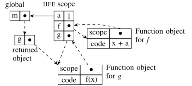
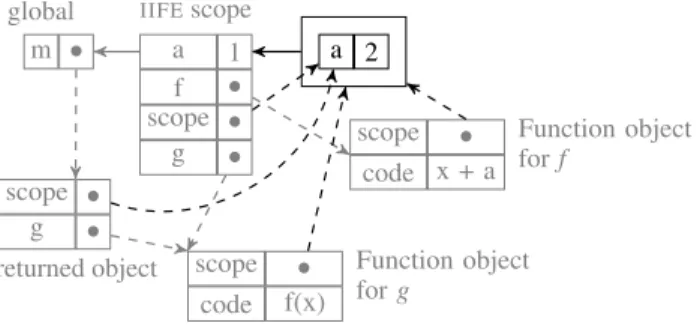
m • global a 1 f • g • IIFEscope g • returned object scope • code x + a Function object for f scope • code f(x) Function object for g
Figure 1. Scope diagram after executing theIIFEof listing 1.
its argument to the value of the variable a. When we call m.g(0) from outside of the module, we get 1, which is the value of a.
A diagram of the scopes and objects created after executing the IIFEand before running the call at line 8 is given in figure 1. In this diagram, JavaScript objects are represented as boxes which contain lines of pairs. A pair is a property, which has a property name in its left cell and a value in its right cell. When the value of a pair is a reference, a bullet is drawn in the cell and an outward dashed arrow points to the referenced object. E.g., the global object has a property named m which refers to the (unnamed) object which has g as its sole property.
We represent scopes as boxes as well, with a solid arrow indicat-ing the outer scope. When an identifier is not found in a scope, the search continues in its outer scope, and so on until no outer scope is defined.
We can now explain the module pattern by looking at figure 1. Before executing the code in listing 1, the global object is empty. When theIIFEis called, it creates a scope we named “IIFEscope” in the diagram. Since theIIFEis defined at the top-level, its outer scope is the global object. Inside theIIFE, three definitions are made: one variable a and two functions, f and g (lines 2–4). When a function is defined, a function object is created. A function object has a code property containing the body of the function, and a scope property which points to the scope it was defined in. This scope property will be used for executing the body of the function when it is called. Before theIIFEreturns, it creates an anonymous object (line 5) which contains a property g referring to the function g inside the module. Note that there are now two references to g in the runtime environment. Finally, theIIFEreturns the anonymous object, which is bound to the variable m in global scope.
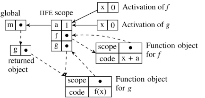
Now, we proceed to explain what happens when the call of line 8 in listing 1 is made (see figure 2). First, the reference m.g is resolved by searching for the m property in the current scope, i.e., the global scope. The global scope does contain an m property which refers to an object, so the interpreter is now searching for a g property inside this object. The g property exists, and refers to a function object, we can proceed with the call m.g(0). When the global scope calls the function referred to by m.g, the interpreter creates a scope for the body of the function called the activation object of g. The activation object contains bindings for each formal parameter of the function. Here, the function g has one formal parameter, x, and the call m.g(0) provided the value 0 as argument. Hence, the activation object of gcontains the property x with value 0. The activation object of g has the scope property of the function object for g as outer scope. Then control is transferred to the body of g. To execute f(x), the interpreter resolves f and x by searching through the scope chain, starting with the activation object of g. The activation object does not contain a property f, but its outer scope does. The reference f is to a function object, so the interpreter can proceed with the call f(x). The property x is found in the activation object, and its value is used to call f. When f is called, the interpreter creates an activation object from the formal parameters of f, and sets the outer scope to theIIFE
m • global a 1 f • g • IIFEscope x 0 Activation of g x 0 Activation of f g • returned object scope • code x + a Function object for f scope • code f(x) Function object for g
Figure 2. Scope diagram for the call m.g(0), line 8 of listing 1.
scope. After that, the interpreter transfers control to the body of f, and executes the code x+a. The interpreter finds the property x on the activation object for f, and the property a on its outer scope. The interpreters substitutes x and a for their values, and returns the value 1by unwinding the stack.
The diagram in the figure 2 serves to illustrate two important facts about the module pattern:
1. The only way for code outside the module to refer to definitions made inside the module is through the returned object. In the example of listing 1, g is the only reference we have access to, but is an alias. Observe that if we were to change the value of m.gby assigning it to another function, m.g = function() { ... }, only the reference m.g would change, but the property g in the IIFEscope would still refer to the original g function. If we want to refer to the declarations inside the module, we need access to theIIFEscope.
2. All functions created inside the module will use theIIFEscope as outer scope. This is just another way to say that functions close over the scope used at the time of their definition (their lexical environment), that is why we also refer to JavaScript functions as closures. If we had access to theIIFEscope, we could change the behavior of functions inside the module by changing the bindings of the scope.
These two facts reveal the importance of theIIFEscope as the central point where binding lookup happens. This is crucial: if we can access the IIFEscope from outside, then we can essentially change the behavior of functions in a very simple way. The next subsection hinges on this point to construct a generic solution to the instrumentation problem.
3.2 Opening the Module Pattern
In the previous subsection, we have seen how the objects and scopes in the module pattern revolved around the scope created by the anonymousIIFE. At this point the only way to access this scope seems to be through the scope property of the exported g function. Unfortunately, this scope property is unreliable: we can easily return a function g that closes over another environment. Consider the following example:
1 var m = (function(){
2 function mkG() { return function g(x) { return x }} 3 return {g: mkG()}
4 }()) 5 m.g(0)
Listing 2. The returned g function does not close over the module scope directly.
On line 3 we associate the return value of the mkG function to the exported g property. The mkG function returns the same g function
m • global mkG • IIFEscope g • Activation of mkG x 0 Activation of g g • returned object code fun... scope • Function object for mkG scope • code f(x) Function object for g
Figure 3. Scope diagram for listing 2.
as in the previous example, but with an important distinction: this gfunction closes over the lexical environment created by the call of mkG. Figure 3 illustrates the difference by the addition of the activation object for mkG which serves as scope for g. We have m.g.scopethat refers to the scope created by mkG, not the scope created by theIIFE. Contrast that with the function f, which closes over theIIFEdirectly. Hence, we cannot rely on the scope property of exported functions to access the inner scope of the module.
Let us now make a simple deviation from the subset of JavaScript we have been using so far. Let us pretend that we can access the scope created by theIIFEby a new scope property of the returned object. We also assume that the scope accessed through this new property behaves like a regular JavaScript object; we can read and write property values on it. We shall see in section 4 how these assumptions can be made true.
1 var m = (function(){ 2 var a = 1 3 function f(x) { return x + a } 4 function g(x) { return f(x) } 5 return {g: g} 6 }()) 7 8 m.g(0) //: 1 9 m.scope.a = 2 10 m.g(0) //: 2
Listing 3. A module exposing its scope.
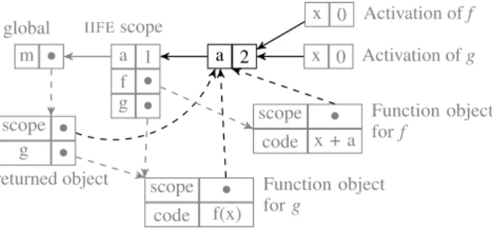
In listing 3, we construct the same module m as in listing 1. When executing m.g(0) on line 8, we still get the result 1. However, this time we have access to the inner scope of the module via the scopeproperty. If we change the value of a inside this scope (line 9), then the call m.g(0) will go find the value 2 bound to a, and that is why we get the result 2 on line 10. Another way to look at it is through the diagram in figure 4. The additional scope property is visible on the returned object referenced by the m property of the global object. This m.scope property points to the scope created by theIIFE, giving read and write access to it. Thus, when we execute line 9, we modify the value of a inside the module; a is associated to the value 2 in the diagram as a result.
By adding this direct reference to the inner scope of the module, we are already able to change the results of the call to m.g, just by changing the value of a variable inside the module. Now, if we want to change the function f outside the module, to return x + 2 ∗ a instead of x + a, we can do so as well. Listing 4 illustrates how on line 4. However, we cannot just write 2 ∗ a, as a is a free variable in this case. We want a to refer to the value of a in the scope of the module. Since we have a reference to the inner scope, we refer to a this way. Hence the call m.g(0) made after the redefinition of f uses
m • global a 2 f • g • IIFEscope x 0 Activation of g x 0 Activation of f scope • g • returned object scope • code x + a Function object for f scope • code f(x) Function object for g
Figure 4. Scope diagram for the call m.g(0) on line 10 of listing 3. The new scope property is highlighted.
the latest definition. By referring to the value of a inside the module, the redefinition of f will always use the dynamic value associated with a. On line 6 we modify a again to the value 2, and the final call to m.g(0) is affected by both modifications to return 4. We are thus able to alter the behavior of m.g by overriding variables and functions inside the module, but writing these changes outside of it. We do not have to touch the module definition to change the result of calls to m.g.
1 var m = (function(){ ... }()) 2
3 m.g(0) //: 1
4 m.scope.f = function(x) { return x + 2 ∗ m.scope.a } 5 m.g(0) //: 2
6 m.scope.a = 2 7 m.g(0) //: 4
Listing 4. Changing the function f and the variable a without altering the module code.
If we can easily override values inside the module, we cannot yet easily undo our changes dynamically. Observe, in the examples above and in figure 4, that by changing the value m.scope.a to 2, we are erasing its previous value. The same is true of the redefinition of f in the last example. If we want to preserve the original values in order to undo our changes, we can do so manually, by putting them in a temporary variable. There is, however, a more elegant solution leveraging the mechanism of property lookup in scopes. The next subsection explains how.
3.3 Layered Scopes for Composability
As we have already seen, a scope has an outer scope. If a property is not found in a scope, the lookup mechanism will follow the outer scope link and continue the search for the property there. The lookup continues in this way until either the property is found, or the outer scope link points to null. Since we want to be able to override bindings in the module without destroying the original values, we can use the lookup mechanism to our advantage.
Let us now change the rules of our JavaScript subset again. We assume that when the module is created, a fresh, empty scope is created as well, which we will call the front scope. The front scope has the scope created by theIIFEas outer scope. Functions defined at the top-level of the module will have their scope property pointing to the front scope. Then, the m.scope property we created in the previous subsection will now refer to this front scope instead of the scope created by theIIFE.
If we now take the exact same code of listing 3 but execute it with the changes of the previous paragraph, we get the situation depicted in figure 5. The new front scope captures the redefinition of ato the value 2 without altering its outer scope. Since both functions fand g defined inside the module have their scope property pointing
m • global a 1 f • g • IIFEscope a 2 x 0 Activation of g x 0 Activation of f scope • g • returned object scope • code x + a Function object for f scope • code f(x) Function object for g
Figure 5. A front scope (highlighted) is added to the module scope. Impacted arrows are highlighted.
to the front scope, when these are called, their activation objects will have the front scope as outer scope. As the lookup mechanism follows the solid arrows from right to left, we see that any property put in the front scope will take precedence over the properties found in the module inner scope. That is why, in the example below, the call to m.g(0) returns 2 right after we change the value of a on line 4. However, we have also gained the ability to undo the change on a by simply deleting the property m.scope.a from the front scope. As the front scope only contained our variation from the base module, the original value of a is never altered. When the value in m.scope.a is deleted, the front scope is empty, and the call m.g(0) will find the property a on the scope created by theIIFE. Hence, after executing line 6, the call m.g(0) now returns the value 1, as if the change to a had never been made.
1 var m = (function(){ ... }()) 2 3 m.g(0) //: 1 4 m.scope.a = 2 5 m.g(0) //: 2 6 delete m.scope.a 7 m.g(0) //: 1
Using the front scope, we are now able to override and delete values inside the module without modifying its code. In a practical setting, we would probably override several properties at once, and would need to delete them all at once. Also, if we are to experiment with different sets of changes, we would like to be able to, e.g., activate one set, then a second one, then deactivate the first one. Using a single front scope is not sufficient for this scenario, but we can put several scopes in front of the module inner scope instead.
Let us make one final addition to our JavaScript subset: the ability to retrieve and change the outer scope of any scope object via the property parent. With this property, we can extend the scope chain used by functions inside the module by putting any number of scopes in front. Since scope objects have a parent link, and we have a reference to the foremost front object (m.scope), then the scope chain is structurally similar to a singly-linked list, with the front scope being the head of the list. Thus we can insert and remove a scope object at any point in the scope chain like we would insert and remove an element in a linked list. The most useful place to insert a scope for instrumentation purposes is between the front scope and the inner scope of the module. Suppose that we have a pushScope(s, chain) function which inserts the scope s into the chain above the front scope; and a companion function removeScope(s,chain)which removes the scope s from the chain. Then we can write the following code:
1 var m = (function(){ ... }()) 2
3 m.g(0) //: 1
m • global a 1 f • g • IIFEscope a 2 f • f • scope • g • returned object
Figure 6. Two scopes are added in front of theIIFEscope. Most references are omitted for legibility.
5 pushScope(s, m.g.scope) 6 m.g(0) //: 4
7 var s2 = {f: function(x) { return −m.scope.a }} 8 pushScope(s2, m.g.scope)
9 m.g(0) //: −2
10 removeScope(s, m.g.scope) 11 m.g(0) //: −1
Listing 5. Composable scopes as layers.
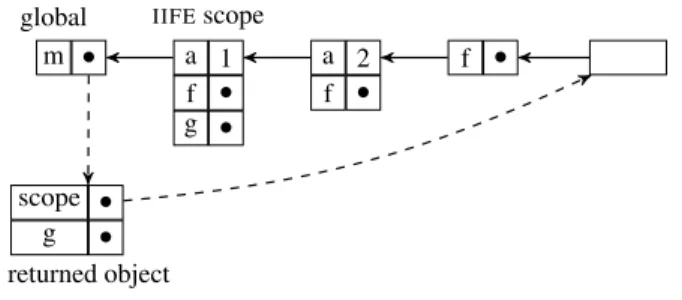
With the module m written exactly like in listing 1, we can add all the changes of the scope object s simply by calling pushScope (line 5). We can add another set of changes, s2 by calling pushScope again. Calling m.g(0) after that will use the f function found in the s2object, and the a defined in the s object, hence the result is -2. Then, we can remove any scope by calling removeScope. On line 10 we remove the first scope added, s; with the binding of a in s gone, the last call m.g(0) uses the value of a found inside the module and the value of f found in the object s2. Figure 6 gives a view of the scope chain when execution reaches line 9. Each set of changes is well isolated from the other, and all sets are linearly ordered, like layers in a cake. Therefore, the precedence of each set of changes is deterministic: the definitions of foremost layers (nearest to the front scope) precede over the definitions on the layers nearest the inner scope module.
The composition we have constructed in this section an ideal solution to the problem of modular instrumentation. We can change the behavior of the module object, without changing one line of code of the module. The changes are written outside the module, and can be put in separate files. Furthermore, we can dynamically toggle sets of changes and compose several of them at once. On the way, we made the following assumptions:
1. that scopes are like standard JavaScript objects: dictionaries we can add properties to, or retrieve property values from; and that JavaScript objects can act as scopes;
2. that a front scope was created by a call to an anonymousIIFE in the module pattern and that we had a reference to this front scope;
3. that we could refer to and modify the outer scope of any scope object.
We did not, however, elaborate on how these assumptions apply to real JavaScript programs. That is the goal of the next section.
4.
The Open Scope Pattern
In the previous section, we made four assumptions about the language we described. In JavaScript, none of these assumptions are true. Fortunately, we can emulate the scope manipulation techniques of the previous section by using two JavaScript constructs: with and prototype delegation. We will create a manipulable scope using
with, and replicate the layer composition examples using prototypes. All the code of this section is standard ECMAScript 5.1, unless otherwise specified.
The with statement is grammatically similar to an if statement. It takes one expression in parenthesis, which evaluates to its binding object, and takes a block of code between brackets. Below is an example of using with. We define a function f in the body of with on line 3. The function f will simply return the value of a. Note that a is free in this context, but calling f on line 5 still returns the value 42. When f is defined, it closes over its lexical environment. As it happens, with defines a lexical environment for the code it wraps, and this environment is based on the binding object, o. Since oassociates a to 42, the call to f will find the binding a and will return 42. 1 var o = {a:42} 2 with (o) { 3 function f() { return a } 4 } 5 f() //: 42
From this example, one may get the wrong impression that with makes the code it wraps dynamically scoped. This is not the case, as the following example demonstrates. In dynamic scoping, free variables are looked up by going through the environments on the stack, rather than going through the lexical environment [7]. Below we call f inside with, so that with creates a lexical environment on the stack when f is called. The call fails to find a binding for a, and an exception is thrown. The function f is not dynamically scoped by being called inside with.
function f() { return a } var o = {a:42}
with (o) { f() } //: ReferenceError: a is undefined
Instead, when a function is defined inside with, it closes over the lexical environment created by with, following standard lexical scoping rules. However, the environment that with creates is special in that binding lookup is delegated to the binding object. The binding object can be dynamic: properties can be added to it or removed from it. Therefore, it is more precise to state that the function f is lexically closed over a dynamic environment. And this is just what we need to open the scope of the module pattern.
In listing 6, we reproduce the example of listing 3 using with to create a reference to the lexical environment of f and g. We create an empty object on line 2 named scope. We then use scope as the binding object of with. In the body of with, we declare the variable aand the functions f and g exactly like in listing 3. The difference from listing 3 comes on line 7, where we export the scope object alongside the function g. On line 11, we call m.g(0), which triggers the call f(0), which returns 0 + a. Since a is defined to be 1 inside the module, the stack unwinds and we obtain the value 1. Now, since we have access to the binding object scope, we override the value aon line 12. The call m.g(0) shows that f will pick the value inside m.scope.aover the one defined in the module, as the returned value is 2.
1 var m = (function(){
2 var scope = Object.create(null) 3 with (scope) {
4 var a = 1
5 function f(x) { return x + a } 6 function g(x) { return f(x) } 7 return {g:g, scope: scope} 8 }
9 }()) 10
m • global a 1 f • scope • g • IIFEscope a 2 scope • g • returned object scope • code x + a Function object for f scope • code f(x) Function object for g
Figure 7. Scope diagram after line 12 of listing 6. The lexical environment created from the with statement and its incoming arrows are highlighted.
12 m.scope.a = 2 13 m.g(0) //: 2
Listing 6. Opening the module pattern using with. It may be surprising that the value in m.scope.a is preferred to the declaration a = 1. After all, the latter is lexically closer to the function f than the beginning of the with statement. While it is true that with creates a scope for the code it surrounds, this scope does not capture declarations. What happens instead is that declarations are captured by the scope of the surrounding function – the function we refer to as theIIFE. Figure 7 reveals the complete picture. The lexical environment created by with is highlighted; it contains the binding object. However, the binding object only contains the property a that we added on line 12. The declarations a, f and g only exist on the activation object for theIIFE. Since the scope property of the function f points to the lexical environment of with, lookup of bindings will start from here, and go up following the solid arrows. The first binding for a on this scope chain is associated to the value 2, and that is why we get the result of line 13.
One can also observe on figure 7 that when the binding object for with is empty, the code inside the module will behave exactly as if with was never used. The only noticeable effect of using with with an empty binding object would be a slight overhead due to the extra scope object when looking up for bindings.
A crucial difference between the situations of figure 5 and figure 7, is that in the former, there is no distinction between the lexical environment and the binding object: they are amalgamated as one scope object. When using with, the environment and the binding object are not the same thing: the environment has an outer scope, but the binding object has no link to the outer scope. In figure 7, the m.scope property points to the binding object of with, while the scopeproperty of the function f points to the lexical environment created by with. The consequence of this distinction is that, while we can override the declarations made inside the module, we cannot referto them from outside via the m.scope property.
We can work around this limitation by creating a parent object for the binding object. This parent object will contain a reference for each declaration made inside the module. The parent object is then assigned as the prototype of the binding object. JavaScript is a prototype-based language: each object has a prototype link to either another object, or null. When looking for a property p in an object that does not contain it, the search continues in its prototype chain until the property is found, or a prototype link points to null. In this respect, property access on a prototype chain mirrors binding resolution in a scope chain.
1 var m = (function(){
2 var scope = Object.create(null) 3 with (scope) { m • global a 1 g • scope • f • IIFEscope f • a 2 a 1 f • g • Parent object scope • g • returned object scope • code x + a Function object for f code x+2*... scope • Function object for f ’
Figure 8. Diagram for listing 7 after line 17. The function object of g is omitted for legibility.
4 var a = 1
5 function f(x) { return x + a } 6 function g(x) { return f(x) } 7
8 var parent = {a:a, f:f, g:g}
9 Object.setPrototypeOf(scope, parent) 10 return {g:g, scope: scope}
11 } 12 }()) 13
14 m.g(0) //: 1
15 m.scope.f = function(x) { return x + 2 ∗ m.scope.a } 16 m.g(0) //: 2 17 m.scope.a = 2 18 m.g(0) //: 4 19 delete m.scope.f 20 m.g(0) //: 2 21 delete m.scope.a 22 m.g(0) //: 1
Listing 7. To make the scope property behave as a reference to the scope of the module, we create a parent object.
In listing 7, we replicate the situation of listing 4 using pro-totypes. The two additions are on lines 8 and 9. First we create the parent object containing one reference for each declaration of the module. Then we set parent as the prototype of scope using the Object.setPrototypeOf method6. Thus, when we redefine f via m.scope.fon line 15, we can now use m.scope.a to refer to the value of a inside the module. If we then override a through m.scope.a to the number 2, this value will have precedence over the module defi-nition of a. This can all be seen on figure 8. The m.scope property refers to the binding object, which contains the overridden values for a and f. If the binding object is empty, then property lookup will happen on the parent object, which mirrors the references of the module scope. Thus, when we delete the properties f then a on lines 19 and 21, the last call m.g(0) returns the same value as the first, non-instrumented one.
It seems that the separation between the lexical environment created by with and the binding object we export as the scope property only leads to the redundant declarations of line 8. Actually,
6This method is part of the ECMAScript 6 standard proposal, though the
non-standard way to set the prototype of objects via the special __proto__ property is available in most ECMAScript 5.1 implementations.
since we have to explicitly write which bindings are exposed, we have gained additional control. Any declaration not present on the parent object cannot be referred to from outside the module. Information hiding can thus still be used when writing the module, even if with surrounds its inner code. Furthermore, since there is no reference to the module scope accessible from client code, the declarations made in the module cannot be altered in any way. Instrumentation code can only alter copies of the module declarations, in the parent object. This guarantees the integrity of the module.
Finally, since the prototype chain of a JavaScript object can also be seen as a linked list, we can realize the idea of layered scopes from subsection 3.3. In listing 8, we recreate the example from listing 5 by defining the function pushLayer(l, chain), which inserts the object l in the given prototype chain; the function removeLayer(l, chain) removes the object l from the given prototype chain (l is not necessarily at the front of the chain). If we then define the module mexactly as in the previous example, we can put all related changes in objects (s and s2), and use pushLayer and removeLayer on the binding object m.scope to change the results of m.g(0).
1 var m = (function(){ ... }()) 2
3 function pushLayer(l, chain) {
4 Object.setPrototypeOf(l, Object.getPrototypeOf(chain)) 5 Object.setPrototypeOf(chain, l)
6 } 7
8 // Assuming l is on the chain for brevity. 9 function removeLayer(l, chain) {
10 while (Object.getPrototypeOf(chain) !== l) 11 chain = Object.getPrototypeOf(chain) 12 13 Object.setPrototypeOf(chain, Object.getPrototypeOf(l)) 14 Object.setPrototypeOf(l, null) 15 } 16 17 m.g(0) //: 1
18 var s = {a:2, f(x) { return x + 2 ∗ m.scope.a }} 19 pushLayer(s, m.scope)
20 m.g(0) //: 4
21 var s2 = {f() { return −m.scope.a }} 22 pushLayer(s2, m.scope)
23 m.g(0) //: −2
24 removeLayer(s, m.scope) 25 m.g(0) //: −1
Listing 8. Using the prototype chain of the binding object to implement the layered scopes of subsection 3.3.
By leveraging the with construct of JavaScript, we have thus been able to replicate all the scope manipulation techniques of the previous section. Consequently, we have produced a working solution to the problem of modular instrumentation, albeit on a trivial example. As the fundamental ingredient of this solution is to access the scope of the module, we refer to the use of with in the way demonstrated in this section as the open scope pattern.
How does the open scope pattern satisfy the four criteria of subsection 2.2? For the separation of concerns, we have certainly been able to write changes to the interpreter outside of it. We could have written the changes in separate files, but did not as the gain would not be obvious on examples of this size. We had to make three changes inside the module: add the with around the inner code, add the scope property to the returned object, and create a parentobject for the binding object. While the first two changes are always the same regardless of the size of the module they are applied to, the creation of the parent object needs to be adapted to
the declarations made in the module. Since we had to change the code inside the module, the open scope pattern may not reach the ideal of the “minimum changes” requirement, but the changes are nonetheless minimal. This pattern is also simple, as it makes use of standard JavaScript constructs. Its only complexity may lie in understanding how with affects scoping rules for the module code; we provided a guiding model through our scope diagrams.
Although we have shown the ability to compose sets of changes as layers, the trivial module we used in the examples of this section may not be convincing enough. In the next section, we apply the open scope pattern to the Narcissus interpreter and evaluate its compliance to the four requirements of modular instrumentation.
5.
Applying the Open Scope Pattern to Narcissus
The Narcissus interpreter follows the module pattern described in subsection 3.1. We are thus able to apply the open scope pattern of the previous section directly. The only lines that need to be added are shown below prefixed by a ‘+’ symbol:
Narcissus.interpreter = (function() { + var scope = Object.create(null); + with (scope) {
...
+ var parent = {globalBase: globalBase, + execute: execute, + getValue: getValue, ...} + Object.setPrototypeOf(scope, parent) return { evaluate: evaluate, ... + scope: scope }; + } }());
The changes are localized to the top and bottom of the file. As the module object already export a few declarations, we just have to add the scope property at the bottom. We also have to expose a few declarations from the module in the parent object. In our instrumented version of Narcissus7, the parent object contains 14 such bindings. With these added lines in place, we are now ready to start instrumenting the interpreter.
5.1 Adding the Faceted Evaluation Analysis
We have seen in the case study of subsection 2.1 that the faceted evaluation instrumentation of Narcissus had three categories of changes. The first of these changes is the addition of state – the program counter – by extending the ExecutionContext object and adding extra arguments to the getValue function. We can now realize this change outside the module by writing the following code:
1 var N = Narcissus.interpreter.scope 2
3 var EC = N.ExecutionContext
4 function ExecutionContext(type, version) { 5 EC.call(this, type, version)
6
7 this.pc = getPC() || new ProgramCounter() 8 }
9
10 ExecutionContext.prototype = Object.create(EC.prototype) 11
12 function getPC() {
7Our version of Narcissus with the open scope pattern is available at
13 var x = EC.current 14 return x && x.pc 15 } 16 17 var GV = N.getValue 18 function getValue(v, pc) { 19 pc = pc || getPC() 20 21 if (v instanceof FacetedValue) 22 return derefFacetedValue(v, pc) 23 24 return GV(v) 25 } 26 27 N.ExecutionContext = ExecutionContext 28 N.getValue = getValue
We start by declaring the shortcut N on line 1 to refer to the exported scope of the interpreter. The original constructor of ExecutionContextis saved as EC on line 3 to be able to refer to it once we have replaced the binding on line 27. On line 4 we define a new constructor for ExecutionContext which calls the original constructor (line 5) and adds the current value of the program counter to this instance. Other properties of the ExecutionContext object are inherited from the original one using the common JavaScript idiom on line 10. On line 18, we define a wrapper to the original getValuethat gets the current value of the program counter pc as an argument, or through a getPC call if the argument was not supplied. This way, the original interpreter can continue to call getValuewithout providing the extra pc argument, but the code of the instrumentation can provide it directly. Finally, we override the bindings for ExecutionContext and getValue in the original interpreter and replace it with our own (lines 27–28).
The second change of the instrumentation is the extension of the executefunction for eachASTnode, in order to split the evaluation of faceted values by calling the evaluateEach function. The execute function is a large (600 lines) switch statement with one case for each AST node type. We follow the same structure by writing a switch of our own on line 3 of the listing below. The faceted evaluation instrumentation does not need to redefine the behavior for all node types, so we wrap the original execute function and delegate to it using the catch-all default of line 14. As in the previous example, we modify the interpreter on the last line. We omit several other case statements for brevity as they follow the same pattern.
1 var EX = N.execute 2 function execute(n, x) { 3 switch (n.type) { 4 case IF:
5 var cond = N.getValue(N.execute(n.condition, x), x.pc) 6 evaluateEach(cond, function(v, x) {
7 if (v) N.execute(n.thenPart, x)
8 else if (n.elsePart) N.execute(n.elsePart, x) 9 }, x)
10 break 11
12 ... 13
14 default: var v = EX(n, x) 15 }
16 return v 17 } 18
19 N.execute = execute
Finally, the third category of changes required by the instru-mentation is the addition of properties to the globalBase object.
This is easily implemented outside the module by creating a new globalBaseobject that inherits from the original one, and defines additional properties.
1 var globalBase = Object.create(N.globalBase) 2
3 globalBase.isFacetedValue = function(v) { 4 return (v instanceof FacetedValue) 5 }
6 7 ... 8
9 N.globalBase = globalBase
However, extending the globalBase object this way is insuffi-cient. In the Narcissus module, the globalBase object is used right after being created to populate the global object for client code. This process happens in the module, before the exports are returned. Therefore, if we try to extend the globalBase object after the mod-ule is created, it will have no effect on the client global object. We could override all the calls made to populate the client code inside the module, but that would lead to a convoluted control flow and obscure code. We rather chose to slightly refactor the module by providing a populateEnvironment function which can be called at a later point, leaving the time for an instrumentation to extend the globalBaseobject. This refactoring involved moving the 30 calls relating to populating the environment into the new function.
There is one final change that required a refactoring, albeit an quite innocuous one. One crucial function, the function that is used by client code to initiate a function call, was created anonymously in the interpreter module. This function having no name, there is no way we could refer to it from outside the module; the open scope pattern can only override values which have identifiers after all. In order to replace this function, we simply gave it a name.
5.2 Evaluation
Separation of concerns The instrumentation of faceted evaluation using the open scope pattern stands in its own file and consists of 440 lines, whereas the original instrumentation totalled 640 lines. Factorization in our instrumentation explains the difference. The changes of behavior brought by the instrumentation can all be grasped by looking at the instrumentation file alone; there is no more feature scattering or tangling. In addition to faceted evaluation, we defined two other analyses: the FlowR tainting analysis [16], and a simple tracing analysis. Both instrumentation could be written in their own file as well.
Minimum changes to the interpreter We added 19 lines to the original interpreter for the open scope pattern (14 lines for ex-posing the bindings), and changed another 32 lines to add the populateEnvironmentfunction and name the anonymous function. 51 lines out of 1300 lines file may not be the minimum, but it is not many. The important insight is that using the open scope pattern still required refactoring inside the module code for the faceted evalua-tion instrumentaevalua-tion. While this refactoring was minor, knowledge of the internal working of the interpreter was nevertheless required. Instrumentation for the FlowR analysis and tracing did not require any change to the interpreter.
Composability The tracing analysis outputs the type of theAST node as they are executed by the interpreter. We are able to activate tracing along with another analysis and obtain helpful debugging output. However, the FlowR analysis and faceted evaluation both override the function call procedure of the interpreter, and are thus incompatible. Activating both at the same time breaks the evaluation of client code. From their specification, it is unclear if the two can in theory be combined, and what the resulting evaluation would
Interpreter Original Refactored Original Refactored + Facets + Facets Mean time 1040.34 1218.77 1215.01 1301.74 Table 1. Mean time (in seconds) it took for each variant of inter-preter to run the test262 suite.
produce. In any case, we can run client code by activating one without the other.
Simplicity The open scope pattern uses only standard JavaScript constructs: with and prototype delegation. The scope manipulations that it produces may not be easy to understand at first, but they are not overly complex. Compared to modifying the semantics of the JavaScript interpreter to enable access to scopes, our solution can be applied to any standard-compliant implementation without any additional library.
We have tested our refactoring of the Narcissus interpreter for correctness using the test262 suite8. The test262 suite contains over
11000 compliance tests for the ECMAScript 5.1 standard. We ran a subset of the suite used for the SpiderMonkey JavaScript engine on both the original interpreter and the refactored one, then we compared their output for each test case. We found both versions to be equivalent. We also ran the tests for the interpreter with the faceted instrumentation activated, and verified that with an empty program counter, the analysis did not alter the semantics of client code.
When running the tests, we also measured the time they took to complete. For each interpreter, the tests were run ten times, on a single thread; all on the same machine. Table 1 shows the arithmetic mean of the times in seconds. The standard deviation was under 10 seconds for all the interpreters. The refactored interpreter, without any instrumentation activated, has an overhead of 17%. This overhead can be attributed to the addition of with alone, as it has a notorious negative impact on performance. However, when we compare the original instrumentation of faceted evaluation with our own, the overhead falls to 7%, indicating that the analysis has a larger performance impact than the open scope pattern. In any case, as Narcissus is written in JavaScript, performance is one order of magnitude slower compared to C++ engines like SpiderMonkey or V8. When running small snippets of code, which take under a second to execute, the overhead of the open scope pattern is not noticeable.
On the other hand, the gain in the ease of writing and debugging analyses is tangible. In order to run the test262 suite with Narcissus, we had to correct a few bugs in its interpretation of JavaScript code. As we fixed those bugs in the original interpreter, we had to port those fixes in our refactored version as well. However, we also had to fix them again in the original faceted instrumentation, but not in our instrumentation of faceted evaluation. Since our instrumentation had minimized the duplication of code, fixing the interpreter bug in the interpreter was enough. This illustrates the benefit of the adequate separation of concerns we achieved.
6.
Discussion
An interface for instrumentation The principal insight of the open scope pattern is that having access to the bindings of the module is sufficient for instrumenting the interpreter from outside. We can view the exported scope property of the open scope pattern as providing a special kind of “protected” interface, in the sense of the protected Java keyword, which allows methods to be overridden by subclasses. As all the bindings of the module are exposed, the
8http://test262.ecmascript.org/
surface of this interface is large, and instrumentations are liable to break at even the slightest internal change made to the interpreter (e.g., any renaming of identifiers). However, we argue that such brittleness cannot be avoided in general. The public interface of a module can be small and robust, but the needs for instrumentation are hard to predict. The practical instrumentation interface should thus be as close to the internal working of the module as possible. The open scope pattern provides a convenient means to build such an interface.
One key construct The functionality of creating a scope that could then be exported and manipulated by instrumentation was essential to the open scope pattern. In JavaScript, this was realized using only one construct: the with statement. Though with is not strictly necessary, to achieve the same effect in standard ECMAScript would require rewriting hundreds of reference and declarations by prefixing them with the scope identifier. Using with is faster, easily undone, and does not affect the readability of the code. It is interesting to note that using with is considered bad practice [5], and is even banned of the strict subset of ECMAScript 5.19precisely because its ability
to change the scope of identifiers is considered detrimental to code clarity and affects performance. We feel that the open scope pattern is a legitimate use case for with, as the alternatives do not satisfy the requirements of modular instrumentation.
Caveats As the open scope pattern relies on overriding identifiers for instrumentation, there are limits to its applicability. First, anony-mous functions cannot be instrumented; they have to be named. We encountered this problem with the faceted evaluation instrumenta-tion in subsecinstrumenta-tion 5.2 for one funcinstrumenta-tion. Second, aliased references must be overridden once for each alias. If the references o and p both point to the same object, and the instrumentation needs to override this object, then we must redefine both references; we have no way to override all aliases at once. We did not run into this issue while writing the instrumentations for Narcissus however. Third, the open scope created by with can only override declarations made at the top level in the module. That is, a declaration made in a lower scope (e.g., local to a function) cannot be instrumented; such declarations would have to be moved to the top level of the module. Again, this has not prevented us from writing instrumentations. Lastly, while the open scope is appropriate to instrument interpreters defined using the JavaScript module pattern, it might not be the most adequate mechanism to use if the interpreter is written in another way. For in-stance, had the interpreter been written in an object-oriented fashion, then inheritance could have been a more straightforward solution.
7.
Related Work
Aspect-Oriented Programming (AOP) The requirements of the problem of modular instrumentation strongly evoke the AOP paradigm [10]. In AOP, we could use predicates (pointcuts) to target specific parts of the code (joinpoints) and provide the new instrumentation behavior that should take over (advices). The FlowR analysis [16] for instance has been applied to the Ruby language using anAOPframework which lowered the complexity of a previ-ous implementation. Achenbach and Ostermann [1] also defined a meta-aspect protocol for implementing dynamic program analyses, and provided a Ruby implementation.
Lerner, Venter, and Grossman [11] implemented anAOPsubset to solve related problem: writing extensions for the Firefox web browser. In their review of Firefox extensions source code, they found that extension writers used any means at their disposal to override the behavior of the browser when no interface was available – including dynamically patching the source code of functions (a practice dubbed “monkey patching”). The authors
report that their language was expressive enough to refactor the extension code without sacrificing functionality. However, their aspect implementation is specific to a Microsoft Research JavaScript compiler and not freely available.
AspectScript [18] is an expressive AOP implementation for JavaScript with advanced scoping strategies, the ability to capture join points inside function bodies, and to intercept reads and writes to variables. AspectScript works by rewriting all client code into reified calls, even code that is not targeted by pointcuts. As its authors note, the transformation multiplies execution time by a factor of 5 to 13, and make debugging the client code rather difficult. The transformation also uses a custom parser that is not up to date with current JavaScript syntax, and can introduce discrepancies with the host JavaScript environment. Finally, AspectScript does not support rewriting JavaScript code that contains with statements.
We initially sought to instrument interpreters for dynamic analy-ses usingAOPtechniques [13], but it turned out that merely using the flexibility of JavaScript was sufficient to solve the problem of modular instrumentation satisfactorily.
Context-Oriented Programming (COP) The composition of lay-ers of subsection 3.3 is reminiscent ofCOP[9]. ContextJS [12] is aCOPextension for JavaScript, that allows layers to refine a class with partial methods. Layers can be toggled dynamically on all or specific instances of the class, and layers can stack, enabling the expressive dynamic redefinition of behavior. However, as the layers of ContextJS can only refine a class and not a function, they are not applicable to the module pattern used by Narcissus.
Other approaches to modular instrumentation We are not alone in trying to improve the process of writing and maintaining dynamic analyses. DiSL [14] is a framework for writing dynamic analyses of Java bytecode using theAOPparadigm. The Jif language [4] which extends Java with information flow functionality uses the extensible Polyglot [15] compiler front-end. However, these approaches target the Java language; it is unclear whether we could reuse their results on JavaScript compilers.
8.
Conclusion
We presented the open scope pattern as a pragmatic means to instrument a JavaScript interpreter for dynamic program analyses. We applied it to the Narcissus interpreter for two information flow analyses: faceted evaluation and FlowR, along with a tracing analysis for debugging; our instrumentations satisfactorily avoided code duplication and feature scattering.
Although we have focused on information flow analyses, we think that the open scope pattern more broadly applies to any behav-ioral variation of code ascribing to the module pattern. Moreover, we feel that the techniques of scope manipulation we described are sufficiently removed from JavaScript peculiarities as to provide a model for applying the open scope pattern to other languages sharing the same dynamic foundations.
References
[1] M. Achenbach and K. Ostermann. “A Meta-Aspect Protocol for Developing Dynamic Analyses”. In: Runtime Verification. Lecture Notes in Computer Science 6418, pp. 153–167.DOI:
10.1007/978-3-642-16612-9_13.
[2] T. H. Austin and C. Flanagan. “Multiple Facets for Dynamic Information Flow”. In: POPL’12. Proceedings of the 39th Annual ACM SIGPLAN-SIGACT Symposium on Principles of Programming Languages. 2012, pp. 165–178.DOI:10.1145/ 2103656.2103677.
[3] N. Bielova. “Survey on JavaScript security policies and their enforcement mechanisms in a web browser”. In: The Journal of Logic and Algebraic Programming82.8 (2013), pp. 243– 262.DOI:10.1016/j.jlap.2013.05.001.
[4] S. Chong, A. C. Myers, K. Vikram, and L. Zheng. Jif Ref-erence Manual. 2009.URL:www. cs . cornell . edu / jif / doc / jif -3.3.0/manual.html.
[5] D. Crockford. JavaScript - the good parts: unearthing the excellence in JavaScript. O’Reilly, 2008.ISBN: 978-0-596-51774-8.
[6] ECMAScript Language Specification (Standard ECMA-262). URL:http://www.ecma- international.org/publications/standards/ Ecma-262.htm.
[7] D. P. Friedman, M. Wand, and C. T. Haynes. Essentials of programming languages (2. ed.)MIT Press, 2001.ISBN: 978-0-262-06217-6.
[8] D. Hedin, A. Birgisson, L. Bello, and A. Sabelfeld. “JSFlow: tracking information flow in JavaScript and its APIs”. In: Symposium on Applied Computing, SAC. 2014, pp. 1663– 1671.DOI:10.1145/2554850.2554909.URL:http://doi.acm.org/10. 1145/2554850.2554909.
[9] R. Hirschfeld, P. Costanza, and O. Nierstrasz. “Context-oriented Programming”. In: Journal of Object Technology 7.3 (2008), pp. 125–151.DOI:10.5381/jot.2008.7.3.a4. [10] G. Kiczales, E. Hilsdale, J. Hugunin, M. Kersten, J. Palm, and
W. G. Griswold. “An Overview of AspectJ”. In: ECOOP 2001 - Object-Oriented Programming, 15th European Conference.
2001, pp. 327–353.DOI:10.1007/3-540-45337-7_18.
[11] B. S. Lerner, H. Venter, and D. Grossman. “Supporting dy-namic, third-party code customizations in JavaScript using aspects”. In: Proceedings of the 25th Annual ACM SIGPLAN Conference on Object-Oriented Programming, Systems, Lan-guages, and Applications, OOPSLA. 2010, pp. 361–376.DOI:
10.1145/1869459.1869490.
[12] J. Lincke, M. Appeltauer, B. Steinert, and R. Hirschfeld. “An open implementation for context-oriented layer composition in ContextJS”. In: Science of Computer Programming 76.12 (2011), pp. 1194–1209.DOI:10.1016/j.scico.2010.11.013. [13] F. Marchand de Kerchove, J. Noyé, and M. Südholt.
“As-pectizing JavaScript Security”. In: MISS’13. Proceedings of the 3rd Workshop on Modularity in Systems Software. 2013, pp. 7–12.DOI:10.1145/2451613.2451616.
[14] L. Marek, Y. Zheng, D. Ansaloni, L. Bulej, A. Sarimbekov, W. Binder, and P. Tuma. “Introduction to dynamic program analysis with DiSL”. In: Science of Computer Programming 98 (2015), pp. 100–115.DOI:10.1016/j.scico.2014.01.003. [15] N. Nystrom, M. R. Clarkson, and A. C. Myers. “Polyglot:
An Extensible Compiler Framework for Java”. In: Compiler Construction, 12th International Conference, CC 2003. 2003, pp. 138–152.DOI:10.1007/3-540-36579-6_11.
[16] T. F. J.-M. Pasquier, J. Bacon, and B. Shand. “FlowR: As-pect Oriented Programming for Information Flow Control in Ruby”. In: MODULARITY’14. Proceedings of the 13th Inter-national Conference on Modularity. 2014, pp. 37–48.DOI:
10.1145/2577080.2577090.
[17] A. Sabelfeld and A. C. Myers. “Language-based information-flow security”. In: IEEE Journal on Selected Areas in Com-munications21.1 (Jan. 2003), pp. 5–19.DOI:10.1109/JSAC. 2002.806121.
[18] R. Toledo, P. Leger, and É. Tanter. “AspectScript: expres-sive aspects for the web”. In: Proceedings of the 9th Interna-tional Conference on Aspect-Oriented Software Development (AOSD’10). 2010, pp. 13–24.DOI:10.1145/1739230.1739233.