Loss analysis of Flyback in Discontinuous Conduction Mode for sub-mW harvesting systems

(1)

HAL Id: hal-01317121

https://hal.archives-ouvertes.fr/hal-01317121

Submitted on 18 May 2016

HAL is a multi-disciplinary open access

archive for the deposit and dissemination of

sci-entific research documents, whether they are

pub-lished or not. The documents may come from

teaching and research institutions in France or

abroad, or from public or private research centers.

L’archive ouverte pluridisciplinaire HAL, est

destinée au dépôt et à la diffusion de documents

scientifiques de niveau recherche, publiés ou non,

émanant des établissements d’enseignement et de

recherche français ou étrangers, des laboratoires

publics ou privés.

Loss analysis of Flyback in Discontinuous Conduction

Mode for sub-mW harvesting systems

Armande Capitaine, Gaël Pillonnet, T Chailloux, Firas Khaled, Olivier Ondel,

Bruno Allard

To cite this version:

Armande Capitaine, Gaël Pillonnet, T Chailloux, Firas Khaled, Olivier Ondel, et al.. Loss analysis

of Flyback in Discontinuous Conduction Mode for sub-mW harvesting systems. NEWCAS, Jun 2016,

Vancouver, Canada. �10.1109/NEWCAS.2016.7604810�. �hal-01317121�

(2)

Loss analysis of Flyback in Discontinuous

Conduction Mode for sub-mW harvesting systems

A. Capitaine

1,2

, G. Pillonnet

1

, T. Chailloux

1

, F. Khaled

2

, O. Ondel

2

and B. Allard

2

1_{Univ. Grenoble Alpes, F-38000 Grenoble, France CEA, LETI, MINATEC Campus, F-38054 Grenoble, France}

2_{Univ. de Lyon, INSA Lyon, Ampère, UMR CNRS 5005, F-69621 Villeurbanne, France}

Abstract—This energy harvesting solution permits the

autonomous supply of low power sensor nodes, without a chemical battery, allowing their extensive use in various environments. The electrical interface between the harvester and the sensor is crucial in order to maximize the harvested energy and boost the voltage to a minimum value required by the sensor. To achieve input impedance and voltage gain independently, this paper presents a flyback converter in discontinuous mode. Using the proposed flyback model validated experimentally, we have studied the impact of each loss source in order to give some trade-off for designing an efficient sub-mW harvesting interface. We underline the effect of the transformer losses due to the magnetic hysteresis as well as the driving loss impact. Following this method, the flyback prototype achieves 71% power efficiency when harvesting from a microbial fuel cell delivering 90µW.

Keywords— flyback design method; energy harvesting; DC-DC converter; maximum power point tracking; microbial fuel cell

I. INTRODUCTION

Harvesting energy from the surrounding environment is an excellent alternative to conventional batteries for powering autonomously remote sensors in addition to processing in an eco-friendly way. Much research currently focuses on harvesting energy from solar, thermal and vibrational sources scavenged from the environment near the sensor. The microbial fuel cell (MFC), although less analyzed in the literature, is a new harvesting technology that exploits the waste materials around the sensor. The catalytic properties of bacteria in some redox reactions can convert chemical energy from a large range of carbonate substrates such as seafloor sediment or compost into electrical energy [1,2]. This energy production is relatively robust and low-cost. However the generated power is around 100µW for cm-scale electrodes and its DC voltage is insufficient e.g. up to 0.7V to power continuously low-power sensor nodes. Therefore, to adapt and store the power generated by the harvester to the sensor, a harvesting interface is required i.e. a DC-DC converter. It has a two-fold objective: i) extract the maximum power from the harvester and ii) boost and regulate the voltage in an intermediate energy storage. Then, the sensor switches between on- and off-states depending on the energy available in this storage. The boost topology is commonly chosen for the harvesting interface [3,4]. However, this architecture suffers from an inherent limitation which is that the maximal power extraction point and voltage gain cannot both be satisfied in one conversion stage even in discontinuous

conduction mode. To overcome this limitation, [4] adds a second stage to adapt the voltage gain independently to the input impedance. However, this two-stage conversion topology limits the achievable efficiency.

[5] proposes to use a flyback in discontinuous conduction mode (DCM) to overcome the limitation of the classical boost converter topology and also offer galvanic isolation adding value in some MFC applications. This work was done for an input power of 10mW. Our paper proposes the study of this topology for a sub-mW power range and presents a design methodology by analyzing each power loss source especially the transformer. The first section briefly presents the harvester electrical model and explains the flyback operation in DCM to show its ability to adapt its input impedance and voltage gain independently. Then, the trade-off for maximizing the power extraction from a sub-mW power source and optimizing the converter efficiency are explained. To help the designer in their choice e.g. transistor sizing, transformer or other components choices, a complete model of the flyback has been given and experimentally validated.

II. FLYBACK CONVERTER FOR MFC ENERGY HARVESTING

A. Harvester electrical model and MPPT

Solar, thermal and biofuel cell harvesters are often

modeled by a voltage source VS and a series resistance RS

(Fig. 1) when operating close to their maximum power point MPP [6]. Identifying these two parameters is a crucial step in

determining the impedance value RIN of the harvesting

interface and so optimizing the power extraction from the harvester. In fact, the power received by the harvesting

interface is maximized when RIN is equal to RS and is

expressed at the MPP as:

𝑃!""=𝑉! !

4𝑅!

(1)

We define the extraction efficiency ηextr as the ratio of the

power delivered to the harvesting interface PIN over the

maximum power the MFC can deliver PMPP. ηextr is equal to

unity when the impedance matching is respected. In the case of our MFC prototypes [7], the MPP is 90µW at 0.3V and their

static behavior can be modeled with VS=0.6V and RS=1kΩ.

The power generated by the MFC cannot be directly used to continuously power low-power sensor node. Therefore, a harvesting interface is necessary to boost the harvester output

(3)

sensor node. The chosen interface must have a global efficiency close to unity regarding the low power at stake. The

global efficiency includes the extraction efficiency ηextr and

the PMU conversion efficiency ηconv (equation (2), Fig. 1)

where the latter is the ratio of the power delivered by the

harvesting interface POUT over PIN.

𝜂!"#$× 𝜂!"#$= 𝑃!" 𝑃!""× 𝑃!"# 𝑃!" = 𝑃!"# 𝑃!"" (2)

Moreover, since the MFC performance depends on the

environment and RS varies, the MPP has to be regularly

recorded to allow a dynamic impedance matching i.e. to

continuously adapt the impedance RIN of the harvesting

interface.

Fig. 1. Harvester electrical model and harvesting interface schematic. B. Flyback converter as harvesting interface

The harvesting interface is commonly realized with a DC-DC converter. The flyback converter working under DCM

is chosen. Its input impedance RIN can be dynamically adapted

to RS by controlling the switching frequency f, without

impacting on the voltage gain α (Fig. 1). Therefore, both conditions i.e. MPPT and output voltage regulation can be respected at the same time. The DCM also reduces the conduction losses in the converter because of the lower average input current. Moreover, the flyback offers a galvanic isolation between the input and output with its two coupled inductors.

The flyback structure is shown in Fig. 2. DCM operation imposes three phases. In the first phase, the MOSFET is

closed and the current in the primary inductance I1 increases

quasi-linearly until a certain I1_MAX. The current in the

secondary side I2 is blocked by the diode. In the second phase,

the MOSFET is open and the energy stored in the primary inductance during phase 1 is transferred to the secondary side. Considering an ideal transformer conversion ratio of 1:1, the

output current I2 is equal to I1_MAX at the beginning of phase 2

and decreases quasi-linearly. Phase 3 starts when I2 reaches

zero and ends when phase 1 is reinstated. An input capacitance

CIN is set to obtain a quasi-constant input voltage VIN and to

smooth the current IIN delivered by the harvester. Regarding

the input current waveform, the flyback impedance can be expressed by equation (3). Supposing the duty cycle D and the

primary inductance L1 are fixed, the MPPT is handled by

varying the frequency accordingly to the MFC impedance RS

fluctuations without changing the voltage gain α.

𝑅!"=

2𝐿!𝑓

𝐷! (3)

Fig. 2. Flyback converter working in DCM as harvesting interface.

At the output, the energy is stored in a capacitance COUT

and is intermittently delivered to the sensor using a hysteresis comparator, shown in Fig. 2, making the output voltage

oscillate between two values VOUT_MAX and VOUT_MIN where

the latter is the minimal voltage required by the sensor. As the

switch is open, energy is being stored in COUT and so VOUT

increases. When it reaches VOUT_MAX the switch closes until

VOUT reaches VOUT_MIN. COUT is chosen so that the amount of

energy stored in one cycle corresponds to the energy

Εsensor_cycle required by one complete cycle of the sensor

(equation (4)). 𝐶!"#= 2𝐸!"#!$%_!"!#$ 𝑉!"!!"# !_{− 𝑉} !"!!"# ! (4)

C. Origin of the flyback power losses

Determining the origin of the power losses in the converter is very important. Regarding the working conditions and electrical devices, the conversion efficiency can be extremely poor especially as the power delivered by our MFCs is less than 100µW. The different power losses of the flyback due to the MOSFET and diode are given in Table. I, considering an ideal transformer with a conversion ratio of 1:1. The MOSFET

presents an on-state resistance RON causing conduction losses

during phase 1 and an internal capacitance COSS causing

switching losses. The diode presents a threshold voltage VD

causing conduction losses during phase 2 and a parasitic

capacitance CD. Although less studied, the transformer induces

non-negligible losses in the flyback especially in sub-mW operation. In the next section, the transformer losses will be modeled in a compact electrical circuit allowing some trade-off between all the flyback losses.

TABLE I. F LYBACK POWER LOSSES

Conduction losses Switching losses

MOSFET 𝑅!" 𝑉! ! 3𝐷𝑅!! 1 2𝐶!""( 𝑉! 2 + 𝑉!"#)!𝑓 Diode 𝑉!𝑉!! 4𝑉!"#𝑅! 1 2𝐶!( 𝑉! 2 + 𝑉!"#)!𝑓 RS VS Harvester IIN VIN RIN Harvesting interface VOUT = αVIN COUT S ens or IOUT !!"#$= !!" !!"" !!"#$= !!"# !!" !!"= !!"×!!" !!"#= !!"#×!!"# !!""= !!! (4×!!) VOUT t VOUT_MIN VOUT_MAX VG t I1 t I2 t I1_MAX D/f (1-D)/f

Phase 1 Phase 2 Phase 3 Phase 1 Phase 2 1:1 VL2 VIN I1 CIN VOUT COUT I2 VG VL1 RS VS S ens or Harvester IIN VDRIVE _I OUT Harvesting interface Hysteresis

(4)

III. FLYBACK DESIGN AND MODELLING A. Component choices

The choice of MOSFET is important because it can induce

conduction losses with RON and switching losses with COSS.

Reducing one (for instance reducing RON by increasing the

drain-source channel width) generally increases the other

(increasing COSS). We confirmed this by using the N-channel

MOSFET FDV301N [8] which was a good tradeoff for sub-mW operation. Its threshold gate voltage is 1V and it has a

capacitance COSS in the order of 90pF, an RON of 3.5Ω and a

total gate charge Qg of 150pC when operating with a VG equal

to 1.5V.

The BAT54 diode [9] was chosen because of its threshold

voltage (lower than 0.3V) and low parasitic capacitance CD of

10pF, thus minimizing the conduction losses in the secondary branch of the flyback as well as the switching losses.

B. Parameter choices

The input capacitance CIN is used to maintain a DC voltage

at the input of the flyback. According to equation (5), its value has to be sufficiently large in order to ensure a negligible input

ripple ΔVIN. We chose to set ΔVIN equal to 1% of VIN.

𝐶!"=_∆𝑉𝑉!" !"× (2 − 𝐷)! 4𝑅!𝑓 = 100× (2 − 𝐷)! 4𝑅!𝑓 (5) The output voltage is set to oscillate around 1.8V with a

ΔVOUT of 0.1V.

If we suppose that the transformer conversion ratio is equal to 1, then the duty cycle D has to be minimized to keep the flyback in DCM as given in equation (6), and maximized to

avoid a large I1_MAX that may drive the transformer to magnetic

field saturation and also induce large conduction losses in the switch. Setting the duty cycle D to 0.5 is therefore a good tradeoff. 𝐷 1 − 𝐷 ≤ 1 √ŋ!"#$× 𝑉!"# 𝑉!" (6)

The switching frequency f and the transformer primary

inductance L1 offer a certain degree of design freedom. To

respect the MPP condition given by equation (3), the {L1;f}

couple is fixed i.e. increasing L1 means decreasing f.

Considering the MFC resistance obtained in section 2

(RS=1kΩ), the influence of L1 i.e. f on the conversion

efficiency ηconv of the flyback converter was evaluated, without

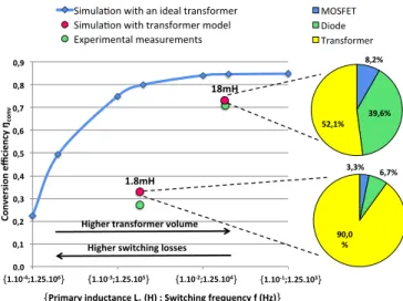
considering the driving loss. The result is the blue curve in Fig. 3. When the inductance is too small (i.e. the frequency is high), the switching losses are mainly due to the fact that MOSFET parasitic capacitance prevails and greatly reduces the flyback efficiency. This result therefore encourages the choice of a frequency close to zero. However, a tradeoff has to be made to avoid the use of a too large transformer in order to limit the circuit to a certain small size.

Our study only considers the MOSFET and diode losses. We will now focus on describing the parasitic aspects that can be encountered in a real transformer and the impact they can

have on the conversion efficiency ηconv.

Fig. 3. Influence of the transformer primary inductance on the flyback conversion efficiency when working at the MPP with an ouput voltage of 1.8V and without considering the driving losses.

Fig. 4. Transformer electrical model. C. Transformer modelisation

The choice of L1 is crucial. Regarding the variation of the

harvester resistance RS, L1 will determine the frequency range

according to the MPPT strategy and thus will greatly influence the conversion efficiency. In order to understand its impact on

the conversion efficiency ηconv, an electrical model is required.

Fig. 4 represents the equivalent electrical circuit of a 1:1

transformer with a primary inductance L1. The copper losses in

the primary and secondary side are modeled with R1 and R2,

the core losses mainly due to the hysteresis of the magnetic

material are modeled by RP, the leakage currents by Lf, the

inter-winding capacitances in the primary and secondary with

C1 and C2, and the capacitance between the primary and the

secondary by C3.

Two transformers from the same manufacturer [10] that are typically used for energy harvesting applications were characterized in order to compare them on the same basis with

different L1 leading to two switching frequencies. The

transformers were characterized using a network analyzer with a frequency range of [5Hz; 30MHz]. The values obtained for both of the characterized transformers (Fig. 4) were evaluated using the modeling strategy described in [11].

0,0 0,1 0,2 0,3 0,4 0,5 0,6 0,7 0,8 0,9

1,E-04 1,E-03 1,E-02 1,E-01

Co nversi on eﬃci en cy ŋco nv Primary inductance L1 (H) 3,3% _6,7% 90,0 % MOSFET Diode Transformer 8,2% 39,6% 52,1% 0,0 0,1 0,2 0,3 0,4 0,5 0,6 0,7 0,8 0,9

1,E-04 1,E-03 1,E-02 1,E-01

Co nversi on eﬃci en cy ŋconv Primary inductance L1 (H) Simula'on with an ideal transformer Simula'on with transformer model Simula'on with transformer model Experimental measurements Experimental measurements 0,0 0,1 0,2 0,3 0,4 0,5 0,6 0,7 0,8 0,9

1,E-04 1,E-03 1,E-02 1,E-01

Co nversi on eﬃci en cy ŋco nv Primary inductance L1 (H) 3,3% _6,7% 90,0 % MOSFET Diode Transformer 8,2% 39,6% 52,1% 0,0 0,1 0,2 0,3 0,4 0,5 0,6 0,7 0,8 0,9

1,E-04 1,E-03 1,E-02 1,E-01

Co nversi on eﬃci en cy ŋco nv Primary inductance L1 (H) Simula'on with an ideal transformer Simula'on with transformer model Simula'on with transformer model Experimental measurements Experimental measurements {1.10-4_;1.25.106_} _{1.10-3_;1.25.105_} _{1.10-2_;1.25.104_} _{1.10-1_;1.25.103_} {Primary inductance L1 (H) ; Switching frequency f (Hz)} Higher switching losses Higher transformer volume 1.8mH 18mH C1 R₁ Rp 1:1 L_f L₁ C2 R₂ L₁ C3 VL1 VL2 Transformer 1 Transformer 2 Ref 78601/8C [10] 78601/9C [10] L1 (mH) 1.8 18 Lf (nH) 155 500 R1 (Ω) 0.35 1.1 R2 (Ω) 0.35 1.1 Rp (Ω) 6 K 30 K C1 (pF) 3 10 C2 (pF) 3 10 C3 (pF) 28 100

(5)

IV. EXPERIMENTAL VALIDATION

A. Transformer model validation and transformer losses

The flyback was simulated by adding the model of each transformer and comparing it to the experimental data. The impedance was accurately matched i.e. the extraction

efficiency ηextr is equal to unity. The conversion efficiencies

are represented in Fig. 3 and highlight an adequate fit between the simulated performances and those acquired experimentally. Our flyback electrical models can thus be considered reliable.

If we take into consideration the previous results with an ideal transformer (blue curve in Fig. 3), the addition of the transformer parasitic elements considerably decreases the converter conversion efficiency. This indicates that the transformer could be the bottleneck to increasing the harvested power efficiency. A previous study on the impact of each transformer parasitic element revealed that the parallel

resistance RP representing the magnetic loss induces the

majority of the transformer losses. This explains the greater losses of the 1.8mH transformer having a parallel resistance five times smaller (6kΩ) than the 18mH transformer (30kΩ).

B. Driving losses

To ensure a self-sufficient process, part of the flyback output power has to be used to supply the MOSFET driver. The

power used to supply the sensor is thus POUT-PG where PG is the

power consumed by the MOSFET driver expressed by:

𝑃!= 𝑄!𝑉!𝑓 (7)

We define the efficiency ηSupply expressed by equation (8),

as the ratio of the power available to supply the sensor

POUT-PG over the maximum power delivered by the MFC PMPP.

𝜂!"##$%=

𝑃!"#− 𝑃! 𝑃!"" =

𝜂!"#$𝜂!"#$𝑃!""− 𝑃!

𝑃!"" (8)

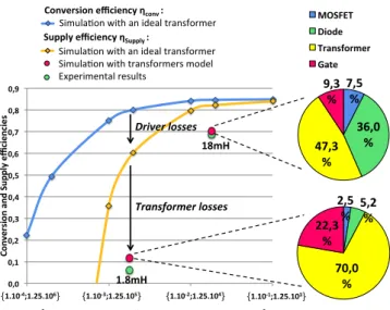
Fig. 5 shows the influence of the driving losses on the power efficiency. The blue curve represents the conversion

efficiency ηconv previously shown in Fig. 3 without considering

PG. The yellow curve represents ηSupply with an ideal

transformer that includes the additional driving losses PG and

highlights the available power given to the sensor. We

observed that the smaller L1, the higher f and the higher the

driving losses PG.

The red dots are the supply efficiency ηSupply simulated with

the two previously characterized transformer models and the green dots are the data acquired experimentally which fit the

simulation well. Using the 18mH transformer, ηSupply reaches

71%. The MPPT is respected and ηextr is equal to unity.

Considering an input power of 90µW, the power that can be used by the sensor is 64µW. The transformer induces almost 50% of the total losses. Hence, to further enhance the flyback performance, the design has to focus on choosing an adapted transformer with very few magnetic losses and an appropriate switching frequency.

Fig. 5. Influence of all the losses onto the flyback efficiency.

V. CONCLUSION

In this paper, we analyzed in detail the losses of the flyback working in DCM for sub-mW harvesting applications. Using the proposed flyback model validated experimentally, we highlighted the impact of the transformer hysteresis losses on the power efficiency and the need to carefully choose the transformer. By choosing a good tradeoff between the switching frequency and the transformer, a prototype was able to transfer 71% of the 90µW maximum power available in the harvester to the sensor with an output voltage of 1.8V.

For more in-depth analysis, other transformers will be studied in the future.

REFERENCES

[1] V. Kiran, B. Gaur, “Microbial Fuel Cell: technology for harvesting energy from biomass”, Reviews in Chemical Engineering. Volume 29, Issue 4, Pages 189–203, Aug. 2013.

[2] S. Venkata Mohan and al. “Microbial fuel cell: Critical factors regulating bio-catalyzed electrochemical process and recent advancements”, Renewable and Sustainable Energy Reviews, 2014. [3] H. Wang, J.-D. Park, et Z. Ren, “Active Energy Harvesting from

Microbial Fuel Cells at the Maximum Power Point without Using Resistors”, Environ. Sci. Technol., vol. 46, no_{9, p. 5247‑5252, 2012.}

[4] J.-D. Park et Z. Ren, “Hysteresis controller based maximum power point tracking energy harvesting system for microbial fuel cells “, Journal of

Power Sources, vol. 205, p. 151‑156, 2012.

[5] F. Khaled, B. Allard, O. Ondel, C. Vollaire, “Autonomous Flyback Converter for Energy Harvesting from Microbial Fuel Cells”, Energy Harvesting and Systems. Nov. 2015

[6] S. Bandyopadhyay and al, “Platform Architecture for Solar, Thermal, and Vibration Energy Combining With MPPT and Single Inductor,” IEEE Journal of Solid-State Circuits, vol. 47, no.9, pp.2199–2215, 2012. [7] T. Chailloux and al. “Autonomous sensor node powered by cm-scale benthic microbial fuel cell and low-cost and off-the-shelf components”, Energy Harvesting and Systems EHS, 2016, in press.

[8] Datasheet of Fairchild Semiconductor, FDV301N Digital FET. [9] Datasheet of Vishay Semiconductors, BAT54.

[10] Datasheet of muRata, 786 Series, General Purpose Pulse Transformers. [11] F. Blache, “Modélisation électronique et électromagnétique d’un

transformateur haute fréquence à circuit magnétique en fonte”, PhD thesis, Institut National Polytechnique de Grenoble, 1995.

0,0 0,1 0,2 0,3 0,4 0,5 0,6 0,7 0,8 0,9

1,E-04 1,E-03 1,E-02 1,E-01

Co nversi on a nd S up pl y eﬃci en ci es Primary inductance L1 (H) 2,5 % 5,2% 70,0 % 22,3 % 7,5 % 36,0 % 47,3 % 9,3 % {1.10-4_;1.25.106_} _{1.10-3_;1.25.105_} _{1.10-2_;1.25.104_} _{1.10-1_;1.25.103_} {Primary inductance L1 (H) ; Switching frequency f (Hz)} Transformer losses Driver losses 2,5% 5,2% 70,0% 22,3% MOSFET Diode Transformer Gate 0,0 0,1 0,2 0,3 0,4 0,5 0,6 0,7 0,8 0,9

1,E-04 1,E-03 1,E-02 1,E-01

Gl ob al eﬃci en cy ŋG LO BAL Primary inductance L1 (H) Simula'on with an ideal transformer: nconv Simula'on with an ideal transformer: ncong-G Simula'on with transformer model: nconv-G Simula'on with transformer model: nconv-G Experimental measurements Experimental measurements 0,0 0,1 0,2 0,3 0,4 0,5 0,6 0,7 0,8 0,9

1,E-04 1,E-03 1,E-02 1,E-01

Gl ob al effici en cy ŋG LO BAL Primary inductance L1 (H) Simula'on with an ideal transformer: nconv Simula'on with an ideal transformer: ncong-G Simula'on with transformer model: nconv-G Simula'on with transformer model: nconv-G Experimental measurements Experimental measurements Conversion efficiency ηconv : Supply efficiency ηSupply : 0,0 0,1 0,2 0,3 0,4 0,5 0,6 0,7 0,8 0,9

1,E-04 1,E-03 1,E-02 1,E-01

Gl ob al eﬃci en cy ŋG LO BAL Primary inductance L1 (H) Simula'on with an ideal transformer: nconv Simula'on with an ideal transformer: ncong-G Simula'on with transformer model: nconv-G Simula'on with transformer model: nconv-G Experimental measurements Experimental measurements Simula'on with an ideal transformer Simula'on with an ideal transformer Simula'on with transformers model Experimental results 0,0 0,1 0,2 0,3 0,4 0,5 0,6 0,7 0,8 0,9

1,E-04 1,E-03 1,E-02 1,E-01

Gl ob al eﬃci en cy ŋG LO BAL Primary inductance L1 (H) Simula'on with an ideal transformer: nconv Simula'on with an ideal transformer: ncong-G Simula'on with transformer model: nconv-G Simula'on with transformer model: nconv-G Experimental measurements Experimental measurements 1.8mH 18mH