Integrated hydrodynamie, waves and plants habitat modeling for restoration of shoreline on Clark Island, Lake St. Francis.

Author Role:

Title, Monographic: Integrated hydrodynamic, waves and plants habitat modeling for restoration of shoreline on Clark island, lake St. Francis

Translated Title: Reprint Status: Edition:

Author, Subsidiary: Author Role:

Place of Publication: Québec Publisher Name: INRS-Eau Date of Publication: 1997

Original Publication Date: Juillet 1997 Volume Identification:

Extent of Work: vii, 48 Packaging Method: pages Series Editor:

Series Editor Role:

Series Title: INRS-Eau, rapport de recherche Series Volume ID: 503

Location/URL:

ISBN: 2-89146-469-9

Notes: Rapport annuel 1997-1998

Abstract: Rapport préparé pour Tecsult Environment Inc.

Call Number: R000503

habitat modeling for shoreline restoration on Clark Island, Lake St. Francis

for shoreline restoration on Clark Island, Lake St. Francis

report prepared for:

Tecsult Environment Inc.

INRS-Eau, rapport de recherche no 503

July 1997

INRS-EAU SCIENTIFIC TEAM

Project Director Michel Leclerc, M.Sc., Dr. Ing., Professor-researcher

Project Manager Jean Morin, M.Sc., Ph.D. student

Specialists Julie Lafleur, M.Sc. research agent Paul Boudreau, M.Sc., research agent Steve Côté, M.Sc. student

TECSULT TEAM

Project Manager Roméo Ciobotariu, Project Engineer Marie-Claude Wilson, Hydraulic specialist Gaétan Thibault,

We thank Ronald Greendale for reviewing the manuscript.

To be cited as :

Morin, J., Lafleur, J., Côté, S., Boudreau, P., Leclerc, M., 1997. Integrated hydrodynamie, waves and plants habitat modeling for restoration of shoreline on Clark Island, Lake St. Francis. For Teesult Environment Ine. INRS-EAU researeh report # 503

Table of contents

2.

2.2. Modeling the hydrodynamics ... 6

2.2.1. Hydrodynamic model ... 6

2.2.2. Discretization ... 7

2.2.3. Initial and boundary conditions ... 9

2.2.4. Calibration and validation ... 9

2.2.5. Integrating the capping structure ... 14

2.3. Results of hydrodynamic modeling ... 16

2.3.1. Reference state: 8200 m3_{/s ... 16}

2.3.2. Average summer flow : 7800 m3_{/s ... 18}

2.3.3. Minimum summer flow : 6 500 m3_{/s ... 19}

2.3.4. Maximum flow : 9 622 m3_{/s, with the capping structure ... 21}

2.3.5. Maximum flow : 9 622 m3_{/s, without the capping structure ... 23}

2.3.6. Impact of the capping structure ... 25

3. Wave modeling ... 27

3.1. Data ... 27

3.1.1. Topography ... 27

3.1.2. Wind statistics and choice of event ... 27

3.2. Modeling the waves ... 27

3.2.1. Wave model HISWA ... 27

3.2.2. Discretization ... 28

3.2.3. Initial and boundary conditions ... 28

3.3. Results of wave modeling ... 28

3.3.1 . Without the capping structure ... 29

3.3.2. Ground-truthing observations ... 29

4. Plants habitat ... 31

4.1. Methodology of plants analysis ... 31

4.2. Field observations and habitat ... 31

4.2.1. Description of abiotic factors ... 33

4.3. Choice of plants for revegetalization ... 34

4.4. Habitat characteristics the capping structure ... 34

5. Analysis of the new capping structure ... 35

5.1. Modification of the capping structure design ... 35

5.1.1. Description of the new design ... 35

5.1.2. Main advantages of the new design ... 36

5.2. Hydrodynamic modeling ... 36

5.2.1. Data ... 36

5.2.2. Modeling the hydrodynamics ... 37

5.2.3. Results of hydrodynamic modeling ... 37

5.3. Wave modeling ... 40

5.3.1. Data ... 40

5.3.2. Modeling the waves ... 40

5.3.3. Result of wave modeling ... 40

5.4. Plant habitat modeling ... 42

5.4.1. Methodology ... 42

5.4.2. Recommendation for revegetalization ... 42

5.4.3. Recommendations for structure amelioration ... 42

6. Conclusions ... 45

List of figures

Figure 1 : Main steps of the methodology ... 2

Figure 2 : Boundaries of the flow domain ... 3

Figure 3 : Six node element used in the discretization ... 7

Figure 4 : Finite element grid of the flow domain ... 8

Figure 5 : Finite element grid in the vicinity of Clark Island ... 8

Figure 6 : Validation results for velocity measurements ... 12

Figure 7 : Depth in the vicinity of Clark Island for the validation of the reference state ... 13

Figure 8 : Velocity in the vicinity of Clark Island for the validation of the reference state ... 13

Figure 9 : Illustration of the capping structure ... 14

Figure 10 : Profile of the capping structure ... 14

Figure 11 : Actual topography of the northwest shoreline of Clark Island ... 15

Figure 12 : Modified topography of the northwest shoreline of Clark Island taking into account the capping structure ... 15

Figure 13 : Depth in the vicinity of Clark Island at a flow of 8 200 m3_{/s ... 17}

Figure 14 : Velocity in the vicinity of Clark Island at a flow of 8 200 m3_{/s ... 17}

Figure 15 : Depth in the vicinity of Clark Island at a flow of 7 800 m3_{/s ... 18}

Figure 16 : Velocity in the vicinity of Clark Island at a flow of 7 800 m3_{/s ... 19}

Figure 17 : Depth in the vicinity of Clark Island at a flow of 6 500 m3_{/s ... 20}

Figure 18 : Velocity in the vicinity of Clark Island at a flow of 6 500 m3_{/s ... 20}

Figure 19 : Depth in the vicinity of Clark Island at a flow of 9 622 m3_{/s with the capping} structure ... 21

Figure 20 : Velocity in the vicinity of Clark Island at a flow of 9 622 m3_{/s with the capping} structure ... 22

Figure 21 : Shear velocity in the vicinity of Clark Island at a flow of 9 622 m3_{/s with the capping} structure ... 22

Figure 22 : Depth in the vicinity of Clark Island at a flow of 9 622 m3_{/s without the capping} structure ... 23

Figure 23: Velocity in the vicinity of Clark Island at a flow of 9622 m3_{/s without the capping} structure ... 24

Figure 24 : Shear velocity in the vicinity of Clark Island at a flow of 9 622 m3_{/s without the} capping structure ... 24

Figure 25 : Differences between velocities simulated with and without the capping structure at a flow of 8200 m3_{/s ... 25}

Figure 26 : Wave induced shear velocities without the capping structure ... 30

Figure 27 : Wave induced shear velocities with the capping structure ... 30

Figure 28 : Field photos of island shore ... ' ... 32

Figure 29 : Illustration of the new capping structure ... 35

Figure 31 : Depth in the vicinity of Clark Island at a flow of 8 200 m3_{/s with the new capping}

structure ... 38

Figure 32: Velocity in the vicinity of Clark Island at a flow of 8 200 m3_{/s with the new capping} structure ... 38

Figure 33 : Shear velocity in the vicinity of Clark Island at a flow of 8 200 m3_{/s with the new} capping structure ... 39

Figure 34 : Differences between velocities simulated with and without the new capping structure at a flow of 8200 m3_{/s ... 39}

Figure 35 : Water depth within the capping structure as introduced in the wave model (created with 8 200 m3/s simulation) ... 41

Figure 36: Wave induced shear velocities with the new capping structure ... 41

Figure 37: Recommendation for revegetalization ... 44

List of tables

Table 1 : Transited discharges for different hydrological events ... 5

Table 2 : Hydrological conditions for the validation reference state ... 9

Table 3 : Measured and calculated discharges for different sections ... 10

Table 4 : Validation results for velocity measurements ... 11

Table 5 : Water level calculated by the hydrodynamic model at different points of interest ... 26

1.

Introduction

This study is part of the Clark Island sediment rehabilitation project. Clark Island is located at the outlet of Lake St. Francis, 1.5 km west of Valleyfield, Québec. The island is currently owned by General Chemical Canada Ltd. (GCCL) ; prior to 1986, it was owned by Allied Chemical, now AlliedSignal, who operated several industrial facilities on the island. In 1986, the Ministère de l'environnement et de la faune du Québec (MEF) requested that AlliedSignal characterize the impacted sediments around the island. Between 1987 and 1993, several sediments characterization studies were conducted by Tecsult. Zone A, located on the northwest shore of Clark Island, has been identified by MEF as the area requiring the most attention because it contains contaminated sediments, mostly pyrite cinders, resulting from AlliedSignal industrial activities. The proposed remediation solution for this zone consists in physically isolating the contaminated sediments with the help of an engineered cap.

Since currents appeared to be the main physical factor influencing the site, INRS-Eau was contracted to simulate the hydrodynamics around Clark Island in order to assess the effect of current velocities on the engineered cap and to propose adequate vegetation for the site. However, evidence of relatively important wave-induced erosion suggested that waves were also a control mechanism of substrate variations and plant species distribution. Therefore, INRS-Eau undertook modeling the waves at the site, both in the absence and the presence of the capping structure, in order to better predict future plant distribution and growth.

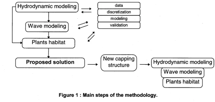
This report investigates the hydrodynamics, the waves and the emergent aquatic vegetation around Clark Island (Figure 1). Hydrodynamic simulations were produced for several flow discharge scenarios. Waves produced by exceptionally strong winds from several directions were simulated and their impacts on the capping structure and on plants were analyzed. A survey of local emergent aquatic plants was conducted and their abiotic preferences were determined. Modifications to the planned capping structure were proposed in order to pro duce a healthy, diversified and stable environment, and an analysis of a new design was performed.

Chapters 2, 3 and 4 of this report were built using the first design of the capping structure: following recommendations, the design was modified by Tecsult to what is called herein the «new design ». This new design is fully analyzed in Chapter 5. Chapter 2 presents the

hydrodynamic simulations, Chapter 3 addresses the modeling and interpretation of wind wave, Chapter 3 analyses the abiotic needs of emergent plants and their distribution. Chapter 5 presents a modified capping structure (new design) which was analyzed for hydrodynarnics, waves and plant colonization.

The main steps of the methodology used in the Clark Island study are described in figure 1.

Hydrodynamic modeling data

---+ +-- discretization modeling

;:::-

f

Figure 1 : Main steps of the methodology.

Wave modeling Plants habitat

Three main topics were considered in order to define an optimized solution for the reintroduction of vegetation at the site. Hydrodynamics, waves and plant habitat are successively analyzed following the same procedure: data collection, discretization of the data, modeling and validation of the results. Only plant habitat assessment has a slightly different work sequence.

Most of the images of this report were produced with the MODELEUR (Secretan et al. 1996), a powerful G.I.S. built specifically for fluvial application. This tool has strong modeling capabilities and works with either triangular or regular rectangular elements for finite element applications, as weIl as for finite difference programs.

2.

Hydrodynamic modeling

2.1. Data

The first step in hydrodynamics modeling is to collect two sets of physical data: a detailed topography of the river reach to be simulated with a description of riverbed materials and aquatic plants, and a reliable stage-discharge relationship at the downstream boundary of the river reach under study.

2.1.1. Topography

The topography of Lake St. Francis is weIl documented. Around 250 000 measurement points, available from the Canadian Hydrographic Service, coyer the entire lake. Almost 100 000 of those points are located in the modelized reach of Lake St. Francis which runs from a transversal section located about 20 km upstream from Clark Island down to the inlet of the Beauharnois canal and to the Coteau hydraulic structures (see figure 2). A detailed topography around Clark Island has also been provided by Tecsult. The topography used for the hydrodynamic simulations is based on RIGL 55. Therefore, the data provided by Tecsult has been converted from RIGL 85 to RIGL 55 (8 cm lower than RIGL 85).

Coteau 3 Gauge station for water level at Coteau-Landin

Upstream boundary

Summerstown .(:?

o

Figure 2 : Boundaries of the flow domain.

2.1.2. Aquatic plants

Submerged aquatic plants must be incorporated in the model for summer and early fall simulations because their occurrence creates significant friction affecting the flow pattern (Morin et al 1996). Seven species are considered abundant, forming 12 distinct vegetation systems distributed all over the lake bottom from very shallow depths to more than 12 m. For the hydrodynamic simulations, we used the plant distribution map and the related Manning' s friction coefficient from Morin et al. (1996). This friction coefficient is ca1culated using a function that takes into account the state of annual growth, the relative composition of plant species, their size and their density. Manning's coefficient is then interpolated to the nodes of the finite element grid.

2.1.3. Substrate

Substrate, along with aquatic plants, creates friction along the bottom. Precise spatial distribution of various grain diameters is essential for hydrodynamic modeling. The substrate of Lake St. Francis has been mapped in detail by Morin and Leclerc (in prep) using precise topographie maps of the lake, 16 000 qualitative observation stations from the Canadian Hydrographie Service, 325 sampling stations with granulometric analyses available in the literature and 250 field observations. The map was then digitized and included in the model with the Manning's friction coefficient. For the purpose of the hydrodynarnic simulation, Manning's coefficient «n » was calculated using a mean substrate diameter in accordance with the following equation (Morin and Leclerc, in prep) :

1

-- = 34.9( --log d,)o.31 n

where,

d' = average grain diameter (m).

The average grain diameter was ca1culated for each combination of materials with the following equation :

i=l

where,

di

=

w_i

=

=

2.1.4. Hydrology

(1)

(2)

The data on the hydrological regime of Lake St. Francis (Table 1) was derived from Morin et al. (1994). Lake St. Francis has a mean annual flow of 7 500 m3_{/s, of which more than 95%} originates from Lake Ontario. The maximum monthly flow recorded between 1962 and 1993 is

10 012 m3_{/s (May 1993) and the minimum monthly flow recorded during the same period is 4}

999 m3_{/s (May 1965). Most of the water in Lake St. Francis flows into Lake St. Louis through}

the Beauharnois canal where it is used for power generation. The portion of the flow discharge diverted to the Beauharnois canal is managed by the Coteau control structures; a minimum flow of 290 m3_{/s must be evacuated through those structures at aIl times to maintain acceptable}

environmental conditions.

Since December 1993, Hydro-Québec applies the following policy in operating the Coteau control structures:

• The minimum flow at Coteau 3 between July 16th and April 14th is 200 m3_{/s; from}

April 15th to July 15th it is 300 m3_{/s ;}

• at Coteau 1, the minimum flow is 90 m3_{/s from July 16}th _{to April 14}th _{and 140 m}3_/s

from April 15th to July 15th;

• if the total discharge transiting through the Coteau control structures is less than 1 440 m3_{/s, the flow at Coteau 3 is kept at 200 m}3_{/s or 300 m}3_{/s, depending on the season, and}

the remaining water flows through Coteau 1 ;

• if the total discharge is more than 1 440 m3_{/s, all exceeding flow is split between}

Coteau 1 and Coteau 3.

The water level at Coteau-Landing is usually kept at around 46.42 m - RIGL 55 (RIGL 85: 46.5) in summer and 46.48 m - RIGL 55 (RIGL 85 : 46.56) in winter. However, fluctuations occur (min. : 46.25 m and max. : 46.55 m). This data has been used as a reference to validate the water level of each hydrodynamic simulation.

Table 1 : Transited discharges for different hydrological events Hydrological event

Average summer flow (August) Low summer flow (July) Maximum flow (April)

Transited discharges (m3_/s) Upstream boundary 7800 6500 9622

Coteau control structures 1000

500

2.2. Modeling the hydrodynamics

2.2.1. Hydrodynamic model

The hydrodynamic modeling was performed using the HYDROSIM model developed at INRS-Eau (see Heniche et al. 1997). The approach used is based on the two-dimensional numerical modeling of the shallow water equations, which are solved using the finite element method. It represents the mass and momentum conservation principles, and takes into account the local granulometric assemblage for the bottom friction parametrization. It produces reliable predictions of mean velocity, water level, and discharges for a wide range of hydrologie al conditions. The wetted surface is also solved by the model since it incorporates a drying-wetting capability allowing to estimate the flow boundary dynamically. The theoretical model is represented by the following system:

Mass conservation (3) (4)

a

a

ah 1 a

a

_ax

ay

ay pax

ay

x(x,y)= Cartesian components ; t = time (s);

qx'qy = specifie discharge with regard tox and y (m2_/s); h = water surface level (m);

zf = bed level with respect to a reference plane (m); H = water depth (=h-9 (m);

c = celerity of waves (c = ~ gH) (mis); 3 3. P = density of the water equal to 10 kglm '

u(u, v)= velocity components which are given by the following relationship (mis); u = qxlH (mis)

v =qylH (mis)

Ic

'tij = Reynolds stresses (kg/s2_m)

't: ' 't : = bottom friction in x and y directions (kg/s2_m) 't; , 't; = surface stresses in x and y directions (kg/s2_m)

2.2.2. Discretization

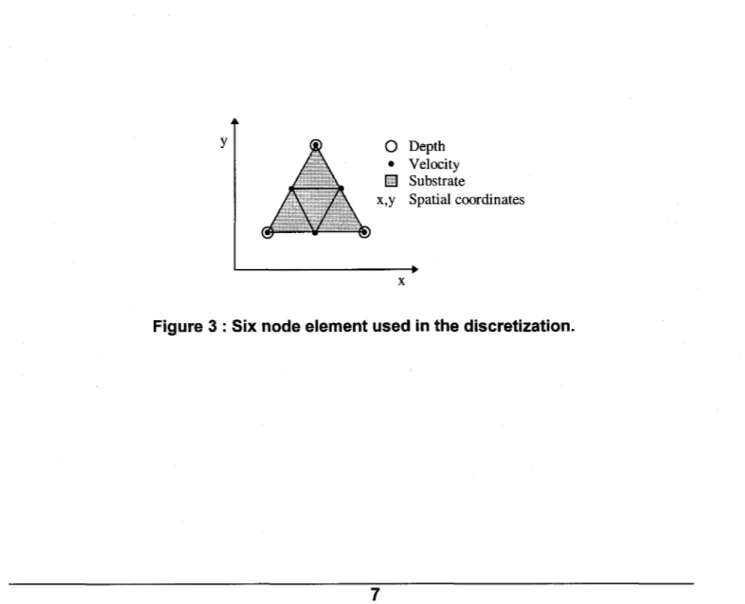
The hydrodynamic model uses a discretization approach based on the finite elements method. The element is composed of six nodes, all involved (linear approximation on 4 triangular sub-elements) to predict the velocities (Figure 3). The geometry and water level only use the three corner nodes to provide a linear approximation of these variables. After discretization, mean velocity, water level and depth can be predicted at every node, or estimated at any point of the flow domain using numerical interpolation.

It involves the subdivision of the flow domain in a number of triangular elements, which size and shape cân be adapted to represent the topographie and substrate variations as closely as possible. The grid is generated automatically with MODELEUR (Secretan et al. 1996). The resulting grid, which supports all the information related to topography, substrate and aquatic plants, is known as the numerical field model (NFM). The grid for the study area in Lake St. Francis comprises 12 217 elements and 25 137 nodes. Figure 4 and 5 present the finite element grid of the modelized reach. A finer grid was constructed for the main channel and for the close vicinity of Clark Island to better represent topographie variations. The mesh size varies from 10 meters in the vicinity of Clark Island to 400 meters in the shallow areas upstream from Clark Island.

y

_o

• Velocity LllI Substrate

x,y Spatial coordinates

x

Figure 4 : Finite element grid of the flow domain.

5{) 100 150 200 (mètres]

2.2.3. Initial and boundary conditions

In this study, steady state conditions were simulated, which did not require special attention to the initial conditions. This implies that the final result for a particular state is independent of the initial conditions. However, the simulation must be sufficiently long to eliminate the errors associated with estimated initial conditions. Either the initial conditions were chosen from the c10sest hydrological conditions already simulated, or a uniform water level, corresponding to the average water level of the flow domain at the discharge considered, was specified.

Boundary conditions can be given as a global discharge, water level or distributed specifie discharge. The c10sed lateral river boundaries were specified as having null tangential and normal velocities. The total river discharge was specified at the upstream boundary and the discharges at the Coteau control structures 1 and 3 were stated as downstream boundary conditions for each simulation. The water level was specified at the Beauharnois canal.

2.2.4. Calibration and validation

Calibration consists essentially in adjusting the value of the flow resistance parameters, i.e. the Manning's bottom frietion coefficient n, and the turbulent viscosity Vt. Since the Manning's n

value was calculated with an already calibrated relationship (equation 1), there were only slight adjustments to be made. For tbis study, a constant turbulent viscosity of 15 m2_{/s was retained.}

The validation reference state corresponds to the event of October 1 st and October 2nd 1996, on which days sorne velocity measurements (N=36) were taken by Tecsult. The river hydrological conditions on both days along with the values used as boundary conditions for the validation simulation are presented in Table 2.

Table 2 : Hydrological conditions for the validation reference state

Variable Event considered

October 1 st October 2nd Validation

Discharge at the upstream boundary nId 8300 m3

/s 8200

Discharge at Coteau 1 control structure 351 m3_{/s 428 m}3_{/s 350}

Discharge at Coteau 3 control structure 200 m3_{/s 200 m}3_{/s 200}

Water level at Beauharnois canal (m~ (1) nId nId 46.36 (46.44)

Water level at Coteau-Landing (m) (1 46.42(46.50) 46.42(46.50) 46.42 (46.50) (lJThe value in parentheses correspond to a RIGL 85 reference whereas ail other water level given in this table are based on RIGL 55. The difference between the two values is 8 cm.

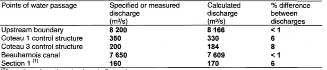
Since discharges had been measured for a few sections on October 1 st and 2nd, this data was also used to validate the hydrodynamic model. The comparison between measured and calculated discharges is presented in table 3. The errors observed are small and negligible, having no signifieant influence on the depth and the velocities simulated near the capping structure.

Table 3 : Measured and calculated discharges for different sections Points of water passage Specified or measured

discharge (m3_/s) Upstream boundary 8 200 Coteau 1 control structure 350

Coteau 3 control structure 200 Beauharnois canal 7 650

Section 1 (1) 160 (l)Location of sections is given in figure 6.

Calculated discharge (m3_/s) 8166 330 184 7609 170 % difterence between discharges <1 6 8 <1 6

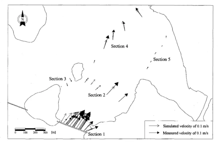
Differences between measured and calculated velocities were established for aIl measures available (Table 4). Overall, 78% of the velocity predictions were within 0.05 mis of measured values. In this particular case, the precision of the current meter is not known ; however it is usually around 0.03 mis. Greater differences in section 1 may be attributed to the fact that the bridge, close to which all measurements for this section were made, was not explicitly considered in the hydrodynamic simulations. Indeed, bridge piles may be responsible for local current phenomena. Figure 6 illustrates the velocity measurements taken by Tecsult compared with the calculated velocities. The orientation given to the measured velocities was based on the orientation of the calculated velocities for each measurement, since directions of the measured velocities were not available. Figure 7 and 8 show the depth and the velocity pattern for the validation reference state.

Table 4 : Validation results for velocity measurements.

Velocity (mis)

NO(1) _{Measured Calculated Differences}

Section 1 1 0.130 0.074 -0.056 2 0.130 0.114 -0.016 3 0.150 0.156 0.006 4 0.130 0.159 0.029 5 0.200 0.164 -0.036 6 0.160 0.167 0.007 7 0.140 0.174 0.034 8 0.160 0.180 0.020 9 0.110 0.181 0.071 10 0.200 0.182 -0.018 11 0.170 0.182 0.012 12 0.120 0.178 0.058 13 0.120 0.164 0.044 14 0.000 0.161 0.161 15 0.110 0.154 0.044 16 0.080 0.150 0.070 17 0.050 0.127 0.077 18 0.020 0.097 0.077 Section 2 1 0.120 0.112 -0.008 2 0.170 0.112 -0.058 3 0.030 0.066 0.036 4 0.020 0.064 0.044 5 0.040 0.057 0.017 Section 3 1 0.040 0.015 -0.025 2 0.030 0.019 -0.011 3 0.000 0.011 0.011 Section 4 1 0.110 0.085 -0.025 2 0.090 0.099 0.009 3 0.100 0.092 -0.008 4 0.140 0.089 -0.051 5 0.020 0.028 0.008 Section 5 1 0.040 0.022 -0.018 2 0.040 0.014 -0.026 3 0.050 0.020 -0.030 4 0.050 0.015 -0.035 5 0.020 0.024 0.004

\

r '

!

\0/ /'

/

/

o 100 200 300 [ml _{----. Measured velocity ofO.l mis}

Depth [ml • 0 • 0.2

~

•

1

6:8

Figure 7 : Depth in the vicinity of Clark Island for the validation of the reference state.

Velocity [mis] . 0 • 0.02 • 0.04 • 0.06 • 0.08 • 0.10 . 0.12 ~ 0.14

o

2.2.5. Integrating the capping structure

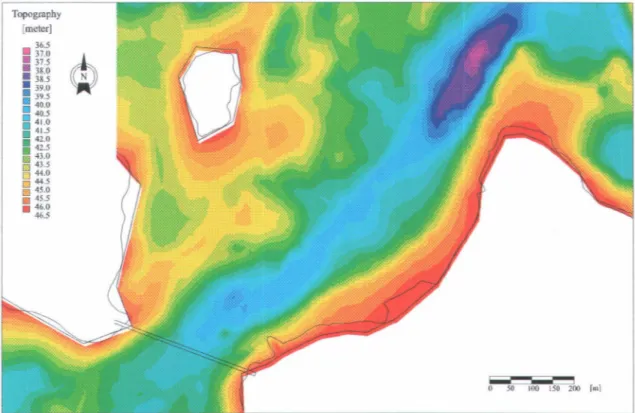
The topography around Clark Island was modified in the numerical field model (NFM) in order to take into account the capping structure (Figure 9, 10, 11 and 12). The elevation of the capping

structure was set at 46.32 m - RIGL 55 (RIGL 85 : 46.40). A regular slope was given between the breakpoint on the capping structure and the topography at the lowest point of the capping structure.

Lower limit of the

capping structure----~J

Zone of interpolation

Figure 9 : Illustration of the capping structure.

Elev. 46.42 (RIGL 85 : 46.50) (RIGL 85 : 46.40)

Breakpoint Zone of interpolation

Lower limit of the capping structure

Topography [meter] . 36.5 . 37.1) ~ . 37.5 . 38.0 . 38.5 . 39.0 Il J9.5 . 40.0 . 40.5 . 41.0 . 41.5 . 42.0 . 42.5 lin 43.0 D 43.5 0 44 .0 0 44.5 ~ 45.0 III 45.5 . 46.0 46.5 o 50 100 ISO 200 fm]

Figure 11 : Actual topography of the northwest shoreline of Clark Island. Topography [meter] . 36.5 • 37.0 ~ . 37.5 . 38.0 . 38.5 . 39.0 . 39.5 . 40.0 . 40.5 . 41.0 . 41.5 . 42.0 . 42.5 m 43.0 D 43.5 0 44 .0 0 44 .5 [ j 45.0 III 45.5 . 46.0 46.5 o 50 100 150 200 lm:

2.3. Results of hydrodynamic modeling

Hydrodynamic simulations were conducted for four distinct events.

• Reference state of October 1 st with the capping structure: 8 200 m3/s (550 m3/s at the Coteau

control structure) ;

• Average summer flow (Morin et al. 1994) with the capping structure: 7 800 m3_{/s (1000 m}3_/s

at the Coteau control structure) ;

• Minimum summer flow with the capping structure: 6500 m3_{/s (500 m}3_{/s at the Coteau control}

structure) ;

• Maximum flow with the capping structure: 9 622 m3_{/s (4 533 m}3_{/s at the Coteau control}

structure) ;

• Maximum flow without the capping structure: 9 622 m3_{/s (4 533 m}3_{/s at the Coteau control}

structure) .

2.3.1. Reference state: 8200 m3_/s

The boundary conditions specified for the reference state (8 200 m3_{/s) were described in section}

2.2.1. The same conditions were kept for the simulation at that flow value, integrating the capping structure: discharges of 350 m3_{/s and 200 m}3_{/s through Coteau 1 and Coteau 3}

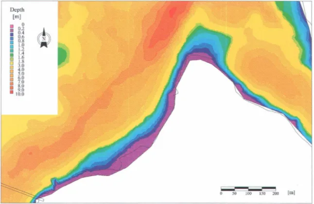
respectively, along with a water level of 46.36 - RIGL 55 (RIGL 85 : 46.44) specified at the entrance of the Beauharnois canal. Figure 13 and 14 illustrate the depth and the velocity pattern for that flow in the vicinity of Clark Island. Vortexes are created above the capping structure and downstream from the capping structure, but the velocities remain fairly small.

Depth [ml Il a • 0.05 • 0.10 • 0.15 • 0.20 • 0.25 • 0.30 • 0.35 • 0.40 • 0.45 .. 1.50 liiI 2.50 II! 3.50 • 4.50 II1II 5.50 '" 6.50 Cl 7.50 ~ 8.50 Il lôj8 50 100 ISO 200 lm]

Figure 13 : Depth in the vicinity of Clark Island at a flow of 8 200 m3_/s.

Velocity [mis] . 0 . 0.02 . 0.04 . 0.06 J;;:J 0.08 • 0.10 . 0.12 Ii:l 0.14 0 0.16 f:!l 0.18 • 0.20 0.22 50 100 ISO 200 rml

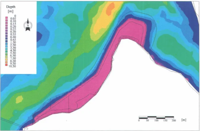
2.3.2. Average summer flow : 7 800 m3_/s

The boundary conditions for the average summer flow of 7 800 m3_{/s were set in order to satisfy}

Hydro-Québec's management policy as described in section 2.1.4. A discharge of 200 m3_{/s was}

specified at Coteau 3 with the remaining 800 m3_{/s flowing through Coteau 1. The water level was}

established at 46.36 - RIGL 55 (RIGL 85 : 46.44) at the Beauharnois canal in order to obtain a

value close to 46.42 - RIGL 55 (RIGL 85 : 46.50) at Coteau-Landing. Figure 15 and 16 represent

the depth and the velocity pattern at that tlow value. A uniform depth of about 10 cm is found on

the capping structure. A discharge of 1000 m3_{/s through the Coteau control structures produces}

velocities up to 0.3

mis

structure are similar to those created at 8 200 m3_/s.

Depth [ml • 0 • 0.05 • 0.10 • 0.15 • 0.20 • 0.25 • 0.30 • 0.35 • 0.40 • 0.45

•

Hg

Velocity [mis] • 0 . 0.05 . 0.10 . 0.15 . 0.20 . 0.25 0 0.30 6l 0.35 il 8:l~ ! i o 50 \IX) 150 200 [ml

Figure 16 : Velocity in the vicinity of Clark Island at a flow of 7 800

m

2.3.3. Minimum summer flow : 6 500 m3_/s

For the minimum summer flow event (6 500 m3_{/s) simulated in this study, the discharge at Coteau}

1 was 300 m3_{/s and the discharge at Coteau 3 was 200 m}3_{/s. The water level specified at the}

entrance of the Beauhamois canal was the same as for the first three simulations, i.e. 46.36 m.

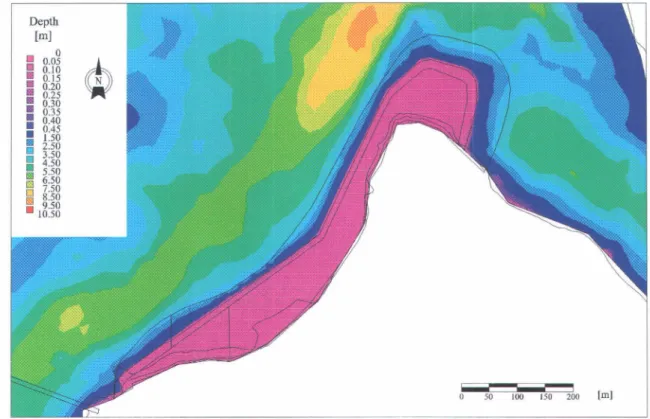
The depth and the velocity pattern are shown in figures 17 and 18. Both the depth and the flow

pattern are similar to the results obtained for the reference state since the discharges at the Coteau

Depth [ml o • 0.05 • 0.10 • 0.15 III 0.20 • 0.25 • 0.30 • 0.35 • 0.40 • 0.45 • _2.50 1.50 !3 3.50 • 4.50 l1li 5.50 '" 6.50 [] 7.50 t;;:) 8.50

•

Figure 17 : Depth in the vicinity of Clark Island at a flow of 6 500 m3_/s.

Velocity [mis] . 0 • 0.02 • 0.04 Il 0.06 • 0.08 • 0.10 • 0.12 m 0.14 [] 0.16 ID 0.18 li 0.20 0.22 50 100 150 2~ [ml

2.3.4. Maximum flow : 9 622 m3_{/s, with the capping structure}

According to Hydro-Québec's management policy, there is a discharge of 2 687 m3_{/s passing}

through Coteau 1 when the flow at the Coteau control structures is 4 533 m3_{/s. Thus the}

discharge at Coteau 3 is 1 846 m3_{/s. The water level at the Beauhamois canal is estimated at}

46.37 m (RIGL 55) at that specifie flow value. As illustrated in figures 19 and 20, the water level

at this particular flow is fairly low in the vicinity of Clark Island, leaving the capping structure uncovered. This can be explained by the fact that the water surface slope has to be rather steep to

allow 4 500 m3_{/s through the Coteau control structures.}

Depth [ml

·

•

Ug

Figure 19 : Depth in the vicinity of Clark Island at a flow of 9 622 m'/s with the capping

Velocity [mis] o . 0.1 . 0.2 . 0.3 . 0.4 III 0.5 m 0.6 Il 0.7 . 0.8 . 0.9 • 1.0 0 1.1 ci 1.2 0 1.3 D 1.4 fil 1.5 • 1.6 1.7 50 100 150 200 [ml

Figure 20 : Velocity in the vicinity of Clark Island at a f10w of 9 622 m3_{/s with the capping}

structure. Shear velocity [mis] . 0 . 0.Q2 . 0.04 III 0.06 • 0.08 . 0.10 !:li 0.12 0 0.14 rJ 0.16 li 0.18 0.20 50 100 150 200 [ml

Figure 21 : Shear velocity in the vicinity of Clark Island at a flow of 9 622 m3_{/s with the}

2.3.5. Maximum flow : 9 622 m3_{/s, without the capping structure}

An additional simulation has been made for a flow of 9 622 m3_{/s in order to analyze the CUITent}

pattern and the shear velocities on the shore of the island in the absence of a capping structure.

Figure 22 illustrates the depth whereas figure 23 illustrates the currents around Clark Island. This

simulation represents flow conditions that are actually relatively rare ; however before the erection

of the Coteau dams, the flow conditions around Clark Island were similar to these simulations.

The shear velocities, which are illustrated on figure 24, reach a value of more than 0.16

mis

Depth [ml • 0 • 0.50 • 1.00 • 1.50 • 2.00 • 2.50 • 3.00 Il 3.50 • 4.00 • 4.50 • 5.00 • 5.50 • 6.00 EllI 6.50 '" 7.00

i3

Figure 22 : Depth in the vicinity of Clark Island at a flow of 9 622 m3_{/s without the capping}

Velocity [mis] g O . 0.1 . 0.2 ~ • 0.3 • 0.4

•

g

:

~

•

l:~

Figure 23 : Velocity in the vicinity of Clark Island at a flow of 9 622 m'/s without the capping structure. Sbear velocity [mis] . 0 . 0.02 . 0.04 . 0.06 . 0.08 . 0.10 III 0.12 0 0.14 ru 0.16 il 8:1~ 50 100 150 200 [ml

Figure 24 : Shear velocity in the vicinity of Clark Island at a flow of 9 622 m'/s without the capping structure.

2.3.6. Impact of the capping structure

The maximum shear stress induced by currents to which the capping structure will be exposed is relatively well represented by the event simulated with a flow of 4 533 m3/s at Coteau structures. Figure 21 presents the distribution of calculated shear velocities in the study area. The maximum value affecting the structure is 0.18

mis

.

The implementation of a capping structure on the northwest shoreline of Clark Island will have a local influence on water depth and velocities. Figure 25 shows the difference between the velocities simulated with and without the capping structure when the total discharge is 8200 m3_/s.

The velocities occurring on the southwestem extremity of the capping structure are increased by

0.05

mis,

that there is no reduction of current velocities within the bay on the eastem side of Clark Island.

Velocity (mis) • -0.07 • -0.06 • -0.05 • -0.04 • -0.03 • -0.02 0 -0.01 III 0.01 Ci 0.02 l'>J 0.03 il 0.04 0.05 ! 1 o 50 100 150 200 [ml

Figure 25 : Differences between velocities simulated with and without the capping structure at a flow of 8200 m3_/s.

Discharges passing through the Coteau control structures have an important effect on water level in the vicinity of Clark Island. Table 5 shows water levels simulated by the hydrodynamic model at different points of interest.

Table 5 : Water level calculated by the hydrodynamic model at different points of interest

Discharge (1) (m3_/s)

Water level calculated (m) (RIGL 55)

Upstream boundary Beauharnais canal Coteau-Landing Capping structure

8 200 (550) 46.60 46.36 46.43 46.40

7 800 (1 000) 46.58 46.36 46.42 46.37

6 500 (500) 46.51 46.36 46.40 46.39

9600 (4 533) 46.51 46.37 46.40 45.96

(1) The value in parentheses corresponds ta the flow passing through the Coteau control structures

The water level at the upstream boundary was determined by the simulations. The first notice able fact observed from the values ca1culated by the model is that the water level at the upstream boundary is the same for both the maximum and minimum flow. The low water level for the maximum flow can be explained by the fact that the gates at the Coteau control structures were open, releasing more water. As a consequence, the portion of the flow diverted to the Beauharnois canal was low compared with aIl other events simulated inducing a more gentle water surface slope.

The water level at the Beauharnois canal was specified as the downstream boundary condition whereas the water level at Coteau-Landing was estimated by the model. The latter value is also· influenced by the discharge diverted to the Beauharnois canal. A low discharge in the

Beauharnois canal for a same total discharge upstream corresponds to a lower level at Coteau-Landing.

According to the simulations for the 9 622 m3_{/s discharge, a high discharge at the Coteau control}

structures has an important local impact on the water level. In fact, the water surface slope created to allow a flow of 4 500 m3_{/s through the Coteau control structures reaches a value of}

3.

Wave modeling

3.1. Data

3.1.1. Topography

Accurate topographie data sets are essential to obtain adequate wave simulations in shallow water. The same data set used for hydrodynamic modeling was also used for wave modeling. Two field elevation models were used ; the first represents the present conditions (without the capping structure) and the second represents the conditions after implementation of the planned capping structure.

3.1.2. Wind statistics and choice of event

Wind statistics performed in Morin et al. (1994) and in an INRS-Eau report on a Lake St.Francis beach stability (Boudreau et al 1995) were used to choose the appropriate wind direction and speed. As reported in Morin et al. (1994), dominant winds in the area are blowing in an East-West direction. They are stronger during the fall and the spring, and there are no extreme winds (45-55 km/h) during the summer. Generally, the stronger winds are westerlies, on an approximately equal frequency from the northwest, the west and the southwest. However during the spring, strong winds can also blow from the east. Statistics from five years of hourly data show that extreme wind speed reached a maximum of 55 kmIh in the area. Extreme winds (45-55 km/h) occur only 5 days per year on average and we believe that 60 kmIh winds represent a rare but «structuring» event, because it can have a significant impact on sedimentation and on resisting material (plants and structure).

For modeling purposes, we elected to simulate a maximum effect of strong winds during the fall. This corresponds to winds blowing from the northwest, the west and the southwest at a speed of 60 km/ho For the Clark Island site, these wind directions have the longest fetches. We also used the calibration event (October 1 st, 2nd 1996) with a total discharge of 8200 m3/s (350 m3/s at Coteau 1 and 200 m3_{/s at Coteau 3) for current and water level conditions as an input to the wind}

model. This event was also simulated with and without the capping structure, allowing to use the same event for wave simulations (with and without the capping structure). Three directions and two bathymetric conditions were simulated for a total production of six wave fields.

3.2. Modeling the waves

3.2.1. Wave model HISWA

Wave models capable of simulating accurately shallow water waves are not common. In the physieal context of Clark Island, strong currents, complex bathymetry and abundant vegetation are affecting wave behavior. Wind growth, wave propagation (refraction) and wave dissipation

parameters of HISWA (illncast Shallow water Wave), a model developed by Delft University of Technology, Netherlands (see Booij et al. 1993).

3.2.2. Discretization

HISW A uses finite differences for ca1culation. Regular rectangular grids are structuring the calculation parameters such as bathymetry, currents, and water levels. Different grids with a different mesh size can be used for data input, calculation and output. Local refinement is done through a «nesting» method that allows to resimulate on a finer grid with known boundary conditions. When done manuaIly, these grids become rapidly fastidious to produce and manage. The MODELEUR was more than useful for grid production, interpolation and visualization. Two different grids were produced for either the situations without and with the capping structure. The first grid that covers a portion the eastem part of the lake is composed of 58 000 nodes with a mesh size of 25 m. A local refinement of the grid, a nesting grid, was built with 64 000 nodes and a mesh size of 5 m. This nested grid covers the capping structure and the surrounding area.

3.2.3. Initial and boundary conditions

For aIl HISW A simulations, boundary conditions were defined mainly by the presence of land. The model was set to take into account white-capping and bottom friction. The width of the direction al sector was fixed at 120 degrees, i.e. 60 degrees on each side of the main direction of propagation. The spectral domain was divided in 90 intervals for a spectral direction al resolution of 1.33 degrees/interval (120/90). Most of the boundaries of the ca1culation grids were limited by land; only the southwestem side was an open boundary. Simulations of southwesterly winds consider a shorter fetch than actually occurs. Considering that the bridges most certainly break the propagation of waves and that the study site is clearly protected by the narrow channel between the islands, we believe that the southwest wind simulation is close to reality.

3.3. Results of wave modeling

The modeling results can be visualized for the three simulated conditions both with and without the capping structure. Wave simulations can produce several output variables ; we have selected the shear velocity created by the orbital movement of waves because it represents the direct effect of waves on structures, on substrate and on plants. In order to simplify the analysis, we have produced two images containing the maximal shear velocity of each node for the three simulations. One node has three attributes of shear velocity produced by the three simulations ; a simple calculation with the MODELEUR allowed us to retain the maximum value for each node of the grid. Thus we obtain two images of the maximal shear velocity which can be observed in the area, one without the capping structure and the other with the structure in place.

3.3.1. Without the capping structure

The modeling results presented in figure 23 show the spatial distribution of the shear velocities produced by waves at the study site. Shear velocity induced by waves is very low in the deep water of the main channel and in the relatively protected area of the bay on the eastern side of Clark Island. Relatively strong shear stress occurs on the northwestern side of the island, at the break in slope and directly on the shore. Maximum shear velocity is 0.8 mis.

3.3.2. Ground-truthing observations

There are no wave measurements available for the area. Thus the quantitative validation of the model is not possible, but sorne qualitative cIues can be gathered in the field. Several field observations along the local shoreline confirm the occurrence of important wave erosion on the northwestern side. On June 17th 1997, we observed significant erosion along the northwestern shore; the root systems of shore trees were severely exposed, tree stumps still in living position were present several meters from the shore, and small but active erosion banks occurred in the northern part of the island. Local substrate distribution also reflects important wave action; cIean sand occurs in the faint bay on the northwest side, coarse material (cobbles and boulders) is present in the northern area.

3.3.3. With the capping structure

The modeling results presented in figure 24 show the spatial distribution of the shear velocity over the planned structure. Differences with the simulation without the capping are very localized, occurring only over the modified zone. Shear velocities in deep water offshore of the island are exactly the same. Shear velocities are significantly smaller on the east side of the island, the capping structure acting as a protective barrier. On the capping structure, the entire energy that was dissipated over aIl of the area is now concentrated on the break in the slope of the structure. This concentration of wave energy induces shear velocity reaching 1.10 m. The energy is almost entirely dissipated after only a few meters over the capping structure; only a small portion is present inside the capping.

Shear velocity [mis] . 0 . 0.10 . 0.20 .. 0.30 0.40 . 0.50 . 0.60 1<'l0.70 00.80 [l 0.90 li 1.00 1.10 50 100 ISO 2~O [ml

Figure 26 : Wave induced shear velocities without the capping structure.

Shear velocity [mis] . 0 . 0.10 . 0.20 . 0.30 0.40 .. 0.50 . 0.60 ~ 0.70 ci O.RO 1:'l0.90 . 1.00 1.10 50 100 150 2bo [ml

4.

Plants habitat

Habitats of emergent aquatic plants are controlled mainly by three abiotic factors: waves, substrate and water depth. Velocities can also play a minor role along with the concentration of nutrients. Waves control the occurrence of plants by exerting a mechanical stress on stems and leaves (Weisner 1991). Water depth is a limiting factor because of the hydrostatic pressure inhibiting the gaseous transportation to the roots and because of the energy necessary for shoots

to reach the water surface (Yamasaki 1984; Spence 1982). Substrate plays two different roles : it

serves as a nutrient pool for plants and it helps stabilize and anchor the rooting system. Nutrient

rich substrates are capable of supporting a larger biomass. Root penetration is essential;

emergent plants are often found on « recently » deposited fine material.

4.1. Methodology of plants analysis

The methodology used for the assessment of emergent aquatic plants is relatively simple and

follows a methodology defined for submerged aquatic plants by Morin et al. (1996). As

mentioned above, abiotic conditions are determinant for species distribution. Very little is known about abiotic preferences of emergent species. Literature data are scarce and allow only for very

broad generalization. In order to understand and describe properly these abiotic preferences, we

conducted a systematic vegetation field survey (identification and distribution). Plant distribution

was mapped, and sediment thickness was measured and its composition was identified.

Combining the distribution of various plant species with the results of wave simulations and of the hydrodynamic model, we were able to calibrate the relative resistance of every species to

wave action and to water depth. It was then possible to predict relatively weIl the future

distribution of plant habitats on the new structure, knowing which plant species would thrive better under various wave energies, water depths and substrate compositions.

4.2. Field observations and habitat

Two field trips were done : a first visit on June 17th to sample plants on the northem part of the

island, and a second visit on July 13th when plants were more developed, flowers were present

and taxonomic identification was easier.

Several species are present in the northeastem part of the island. Figure 28a, taken on July 13t\

shows a wide angle view of the site with most of the species present in the area. From the left

side close to the horizon line, Scirpus lacustris forms a low density community. Immediately to

the right of the Scirpus zone (figure 28a), a dense formation of Typha angustifolia occurs; closer

to shore, Equisetum fluviatile and Scirpus lacustris are present, while on the shore Carex

aquatilis and Scirpus fluviatilis are abundant. On the left side of figure 28, Nymphaea sp. is

Erosion induced by wave action has exposed tree roots, and tree trunks are now observed in the lake. Figure 28c shows the actual onshore vegetation of the northwestem part of the island. Note the very coarse substrate around the point and the absence of emergent plants on this part of the island due to strong wave action.

4.2.1. Description of abiotic factors

We retained five species of emergent plants for which we described their habitat preferences. Table 6 presents the habitat preferences for these species. Although Typha latifolia was not observed in the area, we believe that it will certainly be one of the dominant species of the final design because of its preference for shallow and protected areas.

Table 6: Habitat preferences of selected species

Wave exposure A Water depth B Substrate Simulated wave Simulated

(relative index)

(shear stress Velocities trom 60 km/h (mIs)

wind mls1

Carex 3 -10 cm à 0 cm rich in organic 0.4 to 0.5 less than aquatilis Grows in (average of -5 matter 2 _0.2

~rotected area cm}3 ₁₀ cm to 40 cm

Scirpus 10 10 cm to 140 cm Muddy or sandy 0.5 to 0.7 less than

lacustris Good resistance 10 cm to more 0.2

to wave action than 50 cm

Scirpus 1

o

f1uviatilis Grows in 10 cm and more 0.2

relatively protected area with no current 1

Typha 8 40 cm to 100 cm Fine and rich in 0.3 to 0.5 less th an angustifofia Good resistance organic matter 2 0.2

to wave action 30 cm and more

Typha 0 -10 cm to 40 cm Fine and rich in unknown unknown latifolia Grows in very organic matter 2 probably 0 probably 0

I2rotected area 40 cm and more

A Arbitrary scale based on field observations from 0 (no wave) to 10 (maximum wave)

B Positive values indicate values over the interface roots/stems (soillevel)

1 From Fleurbec, 1987

2 From Couillard et Grondin, 1986 3 From Auclair et al., 1973

In table 6, wave exposure corresponds to field interpretation of the local wave energy. We use an arbitrary scale ranging from 10 for plants occurring in the most energetic environments to 0 for plants growing in protected zones. Water depth corresponds to the distance from the water level (measured positively downward) to the bottom/water interface or soil/air interface. Suitable substrates are mainly rich in fine material and in organic matter. Simulated wave shear stress where plants occur is also used to segregate and quantify field observations. As expected, velocities are relatively low where plants grow. Generally, Scirpus lacustris resists better to wave action and should be used for revegetalization in the area exposed to dominant winds. At the

other end of the spectrum, Typha latifolia grows in shallow water and is neither resistant to CUITent nor to waves and should be used only in protected areas.

4.3. Choice of plants for revegetalization

Several solutions can be proposed for revegetalization of the capping structure. Choosing the best solution depends on the knowledge and the values that are put forward. One of the most recognized values for ecosystem management is the biodiversity concept (see Dodge and Kavetsky 1995). Globally, the larger the number of species sustained by a given ecosystem, the greater the biodiversity. In order to maintain species diversity, habitats have to be diverse in terms of water depth, wave energy and water circulation. Colonizing plants must be a good source of food.

Three species were retained for the revegetalization of the site: Scirpus lacustris, Typha latifolia, and Typha angustifolia, for the following reasons. These plants coyer a wide spectrum of habitat characteristics typical of the study site; they are common on disturbed grounds (especially Typha sp.) ; they are part of the natural ecosystem of the area. These species were also chosen for several qualities other than their habitat tolerance. Scirpus lacustris is an important source of forage for waterfowl and it provides interesting nesting sites for several birds species (Fleurbec

1987). Scirpus lacustris stems and rhizomes are eaten by geese and muskrat ; their seeds are particularly appreciated by waterfowl. Typha latifolia is also an important source of food for waterfowl and mammals.

4.4. Habitat characteristics the capping structure

The most important abiotic variables for emergent plants and therefore for most of other biota were simulated and analyzed for the planned capping structure. As described earlier, emergent plants in this type of environment are mainly influenced by waves, cUITent, water depth and substrate characteristics. Considering that this structure is to be built, the type of substrate available for plants is not relevant because it is possible to plan its nutrient level and its physical properties. As modelized, CUITent velocities are not discriminating for plant species in the sense that the range of speeds within the structure is suitable for all three selected plant species. Waves and water depth appear then to be the controlling factors for plant distribution within the planned structure.

Waves shear stress within the structure is almost the same everywhere ; only the break in slope at the margin of the structure has a different wave energy dissipation. This situation would result in constant abiotic conditions that would favor the growth of a monospecific plant community.

5.

Analysis of the new capping structure

5.1. Modification of the capping structure design

5.1.1. Description of the new design

A new design of the capping structure was produced by Tecsult following recommendations proposed after the first analysis of the local abiotic factors as presented in the first 3 chapters. These recommendations are briefly outlined in the next paragraph. This new is roughly similar in shape to the initial version (Figure 29 and 30). Differences can be summarized in few points: the slope of the edges are slightly steeper, the limit of the structure is partially emergent and the central part of the capping structure is in shallow water.

Emerging ridge Elev: 47 m Actual elevation + 0.3 m ~~~~~7'--~~~- Submerged ridge Elev: 45.5 m ! i o 50 100 150 200 [ml

Elev. 46.42 (RIGL 85: elevation + 0.3

Ridge: Elev. is 45.5,46.2 or 47

Figure 30 : Profile of the new capping structure.

5.1.2. Main advantages of the new design

This new design ha~ severaI advantages in tenus of habitat diversity and sustainability compared to the first one. The most important innovation of this new design is the creation of very diverse abiotic conditions concentrated in a relatively small area.

The presence of emergent «islands » around the structure will protect the internaI part of the structure from ice-scouring, especially during the spring thaw. These emergent breakers can be used by several nesting bird species requiring protected and dry areas. Later, these islands will be naturaIly colonized by shrubs and trees. The occurrence of openings within the emergent structure will favor water circulation and diffusion of wave energy, creating diverse abiotic conditions: zones with relatively important wave energy and currents aIong with more quiet areas. In a long tenu perspective, wave energy is important in order to «c1ean » the structure from organic materiaI, maintaining the potential for fish spawning on the substratum and eliminating the possibility for emergent plants to colonize the entire area, keeping an open water channel within the structure. This basin will favor a better circulation of water within the capping structure which will become a feeding area for fish and juvenile waterfowl.

As suggested earlier, habitat diversity induces species diversity : the new design creates a variety of abiotic conditions that will favor and maintain diversified habitats for plants and fauna. The first design would have resulted, because of the constant abiotic conditions, in a monospecific plant community.

5.2. Hydrodynamic modeling

5.2.1. Data

The new capping structure was integrated in the numericaI field model (NMF) in order to replace the design of the first capping structure. The new elevations of the emergent ridge, the external and internaI slopes of the structure and the amount of materiaIs added in the centraI part of the structure were provided by Tecsult.

5.2.2. Modeling the hydrodynamics

Hydrodynamic simulations were produced with the new capping structure. Simulations were carried out using the HYDROSIM model presented previously in section 2.2.1. The same physical data described in section 2.1 was used along with the same finite element grid (refer to section 2.2.2). Therefore no calibration or validation of the model was necessary for the simulations that were made in this section.

The event chosen to analyze the impact of the new capping structure was the event of October 1 st which has also been used to validate the hydrodynamic model. This event was chosen because of its high recurrence frequency and also because we already had a simulation of the hydrodynamics at this flow with the actual topography, which allowed us to easily analyze the impact of the capping structure on the local currents. These conditions are as follows: the discharge at the entrance of the flow domain (upstream boundary) is 8200 m3_{/s and the discharges at Coteau} control structure 1 and 3 are respectively 350 m3_{/s and 200 m}3_{/s. The water level at the entrance}

ofthe Beauharnois canal (downstream boundary) is 46.36 m - RIGL 55 (RIGL 85: 46.44 m).

5.2.3. Results of hydrodynamic modeling

Results of the hydrodynamic simulation for a discharge of 8200 m3_{/s with the new capping} structure are illustrated by figures 31 to 34. Figure 31 shows water depth as calculated by the model. In general, depth within the structure is relatively shallow, deepest parts are located close to the ridge (figure 31). Note that a more precise topography is presented with wave modeling (Section 5.3). Velocities within the structure are very small less than 0,02 mis (figure 32). Related shear velocities are also small within the structure and reach 0.008 mis in the eastern part (figure 33). Figure 34 presents the difference of velocities between simulation with the new capping structure and present conditions. Theses differences are localized immediately around the new structure.

Depth [ml . 0 • 0.50 • 1.00 • 1.50 • 2.00 • 2.50 iii 3.00

·

₌

Figure 31 : Depth in the vicinity of Clark Island at a flow of 8200 m3_{/s with the new}

capping structure. VeJocity

[mis]

50 100 150 200 [ml

Figure 32 : Velocity in the vicinity of Clark Island at a flow of 8 200 m3_{/s with the new}

Shear velocity [mis] o . 0.002 • 0.004 . 0.006 • 0.008 . 0.010 Il 0.012 . 0.014 . 0.016 III 0.018 r;;] 0.020 00.022 I:J 0.024 f'l 0.026 • 0_0.030 .028 , 1 o 50 100 150 200 [ml

Figure 33 : Shear velocity in the vicinity of Clark Island at a flow of 8 200 m3_{/s with the} new capping structure.

VeJocity [mis] o 0 • -0.01 ~ • -0.02 • -0.03

•

Figure 34 : Differences between velocities simulated with and without the new capping structure at a flow of 8200 m3_/s.

5.3. Wave modeling

Topographical description of the new capping structure (Numerical Field Model) was integrated to the wave model using the MODELEUR, with the same method used for hydrodynamic modeling.

Simulated events are exactly the same in terms of wind speed and direction as in the simulated event of Chapter 3. These wind directions (N-O, 0, S-O) are typical of the area and their speed

(60 kmlh) represents relatively rare conditions. We believed that the se conditions are

« structuring » for plants, sediment and any other resisting material. Water level and current

velocity introduced in the wave modeling were the same as in the event described in Chapter 3. 5.3.2. Modeling the waves

The wave model used is the HISWA model from Delft University (see Chapter 3). This model

uses regular rectangular grid for calculation and for supporting the topographic data (figure 35), water level and currents. The simulations were performed using the same 25 m grid, containing 58 000 nodes, used in Chapter 3. However, because of the interpolation problem caused by the use of this type of grid when it is at an angle with the main structures, we had to refine a nesting

grid over the capping structure that comprises 198 000 nodes with a mesh size of 2 m. Other

conditions like direction al sectors and spectral domain are the same as what was used in Chapter 3.

5.3.3. Result of wave modeling

The result of wave modeling is presented in figure 36. This figure is an integration of three simulations; it is the maximum shear stress ca1culated by the model for each node of the domain in any of the three simulation results. A similar image of the area for the same wind conditions, but without the capping structure, is available in Chapter 3.

The distribution of wave energy is presented in figure 36. The maximum shear stress is located at the margin of the structure where it faces the main wave directions. Within the structure, the wave energy is relatively small, but three areas corresponding to the three openings in the

structure have a relatively high shear stress of 0.4 to 0.6 mis. In protected area, directly located

Depth lm] • 0 m;] 0.25 [] 0.50

o

Figure 35 : Water depth within the capping structure as introduced in the wave model

(created with 8 200 m3/s simulation).

Shcar vc10city [mIs]

.

0