HAL Id: hal-01127772
https://hal.archives-ouvertes.fr/hal-01127772
Submitted on 8 Mar 2015
HAL is a multi-disciplinary open access
archive for the deposit and dissemination of
sci-entific research documents, whether they are
pub-lished or not. The documents may come from
teaching and research institutions in France or
abroad, or from public or private research centers.
L’archive ouverte pluridisciplinaire HAL, est
destinée au dépôt et à la diffusion de documents
scientifiques de niveau recherche, publiés ou non,
émanant des établissements d’enseignement et de
recherche français ou étrangers, des laboratoires
publics ou privés.
PyLayers: An open source dynamic simulator for indoor
propagation and localization
Nicolas Amiot, Mohamed Laaraiedh, Bernard Uguen
To cite this version:
Nicolas Amiot, Mohamed Laaraiedh, Bernard Uguen. PyLayers: An open source dynamic simulator
for indoor propagation and localization. Communications Workshops (ICC), 2013 IEEE International
Conference on, Jun 2013, Budapest, Hungary. �10.1109/ICCW.2013.6649206�. �hal-01127772�
PyLayers: An Open Source Dynamic Simulator
for Indoor Propagation and Localization
Nicolas Amiot, Mohamed Laaraiedh , Bernard Uguen
University of Rennes 1, IETR
Email: {nicolas.amiot, mohamed.laaraiedh, bernard.uguen}@univ-rennes1.fr
Abstract— In this paper, we introduce PyLayers a new open source radio simulator built to tackle indoor localization problem. PyLayers has been designed to simulate complete dynamic scenarios including the realistic movement of persons inside a building, the transmission channel estimation for multiple radio access technologies and the position estimation relying on location-dependent parameters originated from the simulated OSI physical layer. The channel is estimated by using a fast graph-based ray tracing method. From these simulated data, location dependent parameters, such as received power or time of arrival, can be deduced. The realistic movement of persons into the building layout is modeled with a virtual forces approach. The simulated data can be directly used with one of the built-in localization algorithms or be exported to various standards extensions. Finally, the accuracies of both the channel estimation and the localization are compared to measurements and show a good match.
Index Terms— Simulator, propagation, localization,
ray-tracing, multi-wall, mobility model, graph theory
I. INTRODUCTION
E
VALUATING performances of an indoor localizational-gorithm is often a complicate task because performances highly depend on the chosen test environment. Three main ap-proaches are generally retained to perform such an evaluation. First one consists in using statistical models. Those statistical models are very efficient tools for obtaining a global trend of the algorithm accuracy. However, when the simulation scenario becomes very specific, this approach is often not sufficient. For more complex scenarios, a measurement campaign can be realized. The use of measurements is probably the best solution in terms of data quality. In return, it’s also a laborious task in terms of realization and post processing. An interme-diate solution is to use simulators. Simulators are convenient because they combine the accuracy of measurements and ease to use of statistical model. Nevertheless, the accuracy of the simulated data are conditioned by the realism level of the simulator.
Most of available radio estimators such as [1] are efficient in channel estimation but not necessary adapted for localization purposes. The channel impulse response is not directly an input of a localization algorithm. In addition, those tools are generally built for specific bandwidths for a given standard, and this prevent e.g. the validation of heterogeneous local-ization algorithms. Furthermore, movements of persons are generally simulated with random models or more generally by a Markov chain [2]. However, those approaches only capture
the human mobility at a large scale, and don’t take into consideration small scale e.g. attracting points of a room.
The aim of PyLayers [3] is to provide a transversal, ver-satile and upgradable simulator for indoor propagation and localization: Transversal because it addresses multiple simula-tion issues (mechanical, radio, localizasimula-tion); Versatile because each part of simulation is independent and different type of radio access technologies (RATs) are envisaged; Upgradeable because it is an open source project, coded with Python and standard scientific high level libraries Numpy, Scipy, NetworkX and Matplotlib. In the following, the four specific fields of simulation, so-called layers, of PyLayers are presented from section II-A to section II-D. Then, the simulator outputs are shown and compared to measurements in section III.
II. PYLAYERS STRUCTURE:MULTI-LAYERS DESCRIPTION
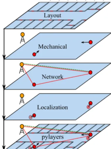
PyLayers is a complete dynamic simulator for indoor propagation and localization based on graphs description. As shown on Fig.1, the simulator is based on four layers: layout, mechanical, network and localization. Each layer regroups various toolboxes and operates independently from each other, but data from each layer can be shared with the others, e.g. the positions computed at the mechanical layer can be used by the network layer.
Layout
Mechanical
Network
Localization
pylayers
Fig. 1: Conception of PyLayers in four independent layers.
A. The Layout layer
The Layout layer allows to precisely describe a simulation scene, in terms of outlines, used materials and radio
propa-gation paths. These layout properties are distributed on four graphs of the layout layer:
• The structure graph Gs(Fig.2) • The graph of rooms Gr (Fig.3) • The visibility graph Gv (Fig.4) • The topological graph Gt(Fig.5)
The structure graph Gsis used to describe the layout outlines
and the materials used in the scene. Conventionally, the nodes with a positive index describes walls, whereas the nodes with a negative index describe vertexes. The edges of Gs link two
nodes with a positive and a negative index respectively. The graph of rooms Grdescribes all the mechanical paths between
the rooms. It is built as a sub-graph of Gs, by retaining only
cycles which possess at least one door. It is especially used by the mechanical layer. The graph of visibility Gv share its
nodes with the structural graph Gs. Its edges link nodes who
share an optical visibility. It is used by the network layer to perform the estimation of location dependent parameters (LDPs). The topological graph Gt contains information about
room connections in term of electromagnetic propagation. Indeed, it allows to fast linking any position inside the layout to Gv. It results from the determination of all the close set
of nodes, , a.k.a. the cycle, of the graph Gs. A complete
description of these graphs is available in [4].
Fig. 2: the structure graph Gs, describes both the outlines of the layout
linking vertexes (hatched circles) and walls (white circles), and the materials of the walls (not represented here).
0 1 2 3 4 5 6 7 8 9 10 11 12 13 14 15 16
Fig. 3: The graph of room Gr describes the possible paths of agents.
1 2 3 4 5 6 7 8 9 10 11 12 13 14 15 16 17 18 19 20 21 22 23 24 25 26 27 28 29 30 31 32 33 34 35 36 37 38 39 40 41 42 43 44 45 46 47 48 49 50 51 52 53 54 55 56 57 58 59 60 61 62 63 64 65 66 67 68 69 70 71 72 73 74 75 76 77 78 79 80 81 82 83 84 85 86 87 88 89 -71 -70 -69 -68 -67 -66 -65 -64 -63-62 -61-60 -59-58 -57-56 -54 -53 -52 -51 -50 -49-48 -40 -23 -22 -2 -9 -8 -7 -6 -5 -4 -3 -1
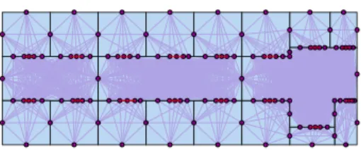
Fig. 4: The visibility graph Gvdescribes all the possible
electromag-netic paths through the layout walls.
B. The Mechanical layer
To ensure dynamic and layer independence, all the up-coming layers processing are based on the SimPy library
0 1 2 3 4 5 6 7 8 9 10 11 12 13 14 15 16
Fig. 5: The topological graph Gt is used to quickly links the Gv
cycles.
[5]. SimPy is a discrete event simulator which allows the simulation of active components. In particular, the mechanical layer uses the Personal Rapid Transit Simulation [6], a SimPy-based library which defines the movement of persons. In PyLayers, persons are called agents. Agents are independent instances moving into the layout. The movement of the agents is implemented by taking into account the 2 of the 3 major properties of the human mobility [7]:
1) Temporal, which defines time dependent action of the movement,
2) Spatial, which defines the physical nature of the move-ment.
The temporal property describes where agents are moving into the layout, e.g. having a target and knowing the path to reach that target. In PyLayers, the target is defined as a room and the path as a succession of rooms. The path from a room i to a targeted room t is obtained with the help of graph Gr.
Rooms i and t corresponds respectively to nodes vi
r and vtrof
Gr. Then, the path is obtained with D, a Djikstra [8] shortest
path algorithm:
Vp= D(vri, v t
r). (1)
The ordered set of node Vpdescribes the shortest path between
vri and vtr. To achieve the complete trajectory from i to t, the
agent go iteratively through all the room corresponding to the nodes of Vp. Hence each time a node of Vp is reached, the
next one becomes an intermediate target it, until the node vtis
reached. With regard to Fig. 3, if the agent is in room i = 1 and its target is room t = 10, the returned path is Vp= {1, 8, 10}.
Thus, the agent will first move from room 1 to its intermediate target 8. Once the agent has reached the center of room 8, it moves to its final target in room 10.
Once the path has been computed, the agents are moving by taking into account the layout environment, such as walls and doors. This is the spatial property of the movement. That spacial property of the human mobility has been modeled using magnetic forces [9]. The magnetic force model aims to obtain a resulting acceleration vector a to drive the agents through the layout. The magnetic force model supposes that the agents and the layout environment can be assimilated to positive poles unlike the intermediates target which can be assimilated to negative poles. Each agent k is potentially under the influence of several magnetic forces: an attractive magnetic force Fit which attracts the agent to its intermediate target
node vit; several repulsive magnetic forces Fr, which avoid
the collision of the agent with the walls or with another agent. According to [9], it is possible to approximate the attractive
magnetic force Fkit on agent k, with the Coulomb’s law:
Fkit≈ qkqit ||Rk,ig||2
ˆ
Rk,it, (2)
with qk and qit the intensities of the magnetic load of the
agent and the intermediate target respectively, Rk,itthe vector
from the agent k to the intermediate targeted node vig. In
order to be close to a human being mobility, we suppose that agents are not grazing the walls. Then the repulsive force must be maximal along the wall . Thus, we propose to model the repulsive magnetic forces Fr with:
Fr(dk,w) =
α ||dk,w||2
ˆ
dk,w, (3)
with dk,w the distance vector from the agent k to a wall w
and α a parameter to adjust the repulsion. Similarly, the inter-agent avoidance can be modeled with (3), by replacing dk,w
by dk,l where k and l are two different agents.
Then, the acceleration vector ak of the agent k with
regard to the environment can be written as the sum of three previously described interactions:
ak= Fkig+ W X w Fr(dk,w) + K X l6=k Fr(dk,l), (4)
where W is the number of walls in the vicinity of the agent k. The vicinity of the agent is determined with a simple distance threshold. The use of that threshold avoids the computation of the forces from all the walls of the entire layout. An example of operation of the mechanical layer can be seen in [10]. C. The Network layer
The network layer describes all radio interactions between the nodes of the entire network, to obtain channel impulse re-sponse (CIR) and/or LDPs. Like the layout layer, the network layer has a graph description. The nodes Vn of network graph
Gn have three attributes: • type: agent or anchor,
• emitted power in dBm,
• receiver sensitivity in dBm.
On the edges of Gn, LDPs between nodes are computed. In
order to manage multiple RATs between nodes, Gn is built as
a multi-graph. A multi-graph is a graph where several parallel edges can link two nodes [11]. This multi-graph description allows to describe each RAT on a different edge of the graph.
1 7 6 1 2 7 6 rat2 rat1
Fig. 6: Example of graph of network Gn which shows all the links
between 4 radio nodes on 2 different RATs. The multi-graph approach can be observed between nodes 1 and 7, which are linked with two different edges.
On each edge are evaluated the received power (Pr) and the time of arrival (TOA) for ultra wide band RAT. Those LDPs
are computed either in real-time with a modified COST-231 multi-wall approach [12], or post processed with the graph-based ray-tracing approach completely described in [13]. The standard COST-231 multi-wall approach consists in evaluating the losses by taking into account the intersection between walls and the ray which link the two nodes. In that model, losses from walls materials are computed supposing a specular incidence angle. The PyLayers multi-wall model adds to that standard model a computation of the losses from the walls by including the incidence angle. Hence, efficient transmission coefficient and excess delay through multi-materials walls can be computed using formulas given in [14]. For the problem at hand, both the incidence angle and the material are required. The incidence angle on each wall is computed during the con-struction of Gvwhile the constitutive materials can be retrieved
using Gs. The received power Pr can be easily evaluated by
subtracting the computed losses from the transmission power. The TOA is obtained by adding the excess delay to the line of sight delay.
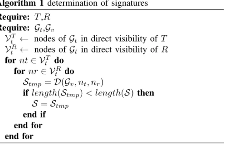
Alternatively, the LDPs can be obtained by a ray-tracing ap-proach from CIR computation. This second apap-proach requires a prior graph-based step: the determination of signatures. These signatures are then used to obtain rays. Let T be a device which tries to obtain LDPs from R, another device. The first step of signature computation consists in obtaining the two set of nodes VtT and VtR which are in direct visibility
of T and R respectively. Then, a shortest path algorithm is computed on Gv for each pair of nodes vTt and vtR of the
set VtT and VtR respectively. The obtained minimal set of
interactions between T and R is the so-called signature S. The procedure is described in Algorithm 1.
Algorithm 1 determination of signatures Require: T ,R
Require: Gt,Gv
VT
t ← nodes of Gtin direct visibility of T
VR
t ← nodes of Gt in direct visibility of R
for nt ∈ VtT do
for nr ∈ VtR do
Stmp= D(Gv, nt, nr)
if length(Stmp) < length(S) then
S = Stmp
end if end for end for
Obtaining CIRs using this approach requires to evaluate a numerous number of rays in Gv. This computation is high time
consuming and provide to obtain the LDPs in real time. On the other side, LDPs obtained from CIRs are more accurate than those obtained by multi-wall technique. The user can choose between the two approaches, depending on its final application.
D. The Localization Layer
The localization layer exploits the LDPs computed by the network layer to perform position estimation. Two types of
methods have been implemented in the localization layer: Algebraic based methods [15] and geometric based method [16]. The algebraic methods are based on maximum likelihood or on a weighted least square estimation to perform. The geometric based method use LDPs to build bounded regions of space called constraints. The geometrical intersection of those constraints define a smaller bounded region which contains the sought position.
III. SIMULATOR OUTPUTS
PyLayers provides numerous useful outputs and visualiza-tion tools for data post-processing and localizavisualiza-tion analysis. From each layer, relevant information can be exported in standard format file (csv, Matlab). Hence, from the mechanical layer, a time-stamped log file is stored for each agent. It contains the position, the velocity and the acceleration vectors. That time-stamped exportation is also available for the LDPs of the network layer and the estimated positions of the localization layer.
The visualizations tools of PyLayers take advantage of the multi-graph description. If Figures 2-6 shows layout description graphs, further visualization tools are available. For instance, the transmission and reflection coefficients of each material from each part of Gs can be displayed. Fig.7
shows the modulus and the phase response of the transmission coefficients for a wood door as a function of the frequency. This standard PyLayers output can also be produced for walls with multiple stack of materials.
1.0 1.5 2.0 2.5 3.0 3.5 4.0 4.5 5.0 fre que ncy (GHz)
0.50 0.55 0.60 0.65 0.70 0.75 0.80 0.85 0.90 0.95 T _|_ T // 1.0 1.5 2.0 2.5 3.0 3.5 4.0 4.5 5.0 fre que ncy (GHz)
4 3 2 1 0 1 2 3 4 T _|_ T // Modul us Phas e
Material : WOOD Thickness : 0.5 cm
Fig. 7: Modulus and phase of transmission coefficient for a wood door as a function of the frequency.
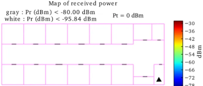
As explained previously, these transmission coefficients are used by the multi-wall algorithm to estimate Pr and TOA. The coverage tool extends the computation from a single link to the whole layout, and thus provides a map of either the received power (Fig.8), or the excess delay (Fig.9). The received power map in addition of received power value may also provide information on areas under the receiver sensitivity and areas under the noise floor. The map of excess delays informs about the delay introduced by the walls contributions.
The accuracy of CIRs obtained using PyLayers can be observed on Fig.10 which compares measurements from [17] and simulations along the same trajectory. Here, CIRs are stacked for each measurement point from bottom to the top of the figure. The figure shows that the most contributing
Map of re ce ive d powe r white : Pr (dBm ) < -95.84 dBm 78 72 66 60 54 48 42 36 30 d B m gray : Pr (dBm ) < -80.00 dBm Pt = 0 dBm
Fig. 8: Map of received power. The black triangle is the transmitter position. The white area represents power under the noise floor, the grey area represents power under receiver sensitivity, elsewhere is the received power in dBm
Map of LOS e xce s s de lay, polar orthogonal
0.0 0.6 1.2 1.8 2.4 3.0 3.6 4.2 4.8
Fig. 9: Map of LOS excess delay. The white triangle is the transmitter position. The degraded colors represent the delay in nsintroduced by the walls in addition of the LOS delay.
paths are retrieved in simulations with a correct delay. This is especially observable for the first arriving path which is mandatory for an accurate TOA estimation. However, it is noticeable that simulations provide a lower density of paths. This is due to the number of interactions considered during the simulation and the ignoring of pieces of furniture in the layout description.
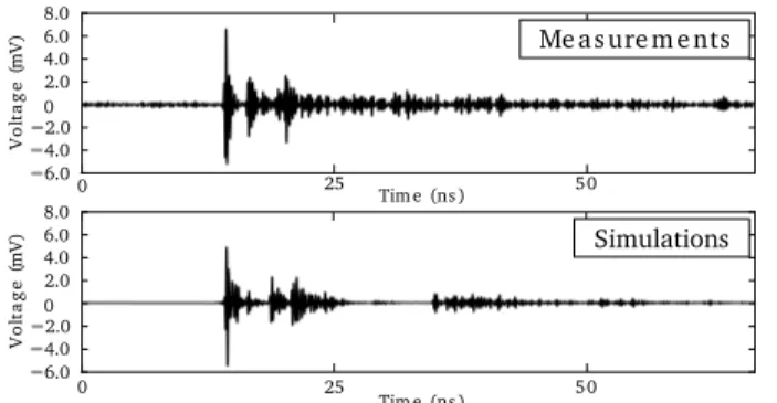
By focusing on a single CIR on Fig 11, it is confirmed that most of the paths and especially the first NLOS path are correctly estimated in terms of delay and amplitude. However, on the simulated plot, a lack of signal can be observed between
Fig. 10: Comparison of Measured (on the top) and Simulated (above) CIRs along an indoor trajectory.
0 Tim e (ns ) 6.0 4.0 2.0 0 2.0 4.0 6.0 8.0 V o lt a g e ( mV) 0 Tim e (ns ) 50 25 50 25 6.0 4.0 2.0 0 2.0 4.0 6.0 8.0 V o lt a g e ( mV) Me as ure m e nts Simulations
Fig. 11: Example of measured and simulated CIRs.
25 ns and 35 ns. This difference is due to a simulation setup which limit the number of considered multi-paths. Increasing the number of paths would increase the computation time but would allow to better fit with the measurements.
IV. CONCLUSIONS
This paper has presented an overview of PyLayers, an open source dynamic radio simulator for indoor propagation and localization. The simulator is built as a stack of specific capabilities named layers. Each Layer takes advantage of a graph description to simulate the realistic movement of persons, to model the propagation channel, and to perform localization estimation. A comparison against realistic mea-surements has shown that the simulator is able to provide accurate CIRs and LDPs. Our current work consists in both improving the global computation speed, and add localiza-tion layer visualizalocaliza-tion tools. Future work consists in adding the OSI MAC layer mechanisms. Finally, due to the open source aspect of the project, we also invite any interested person to use, test, or propose improvements of any parts of the project, by forking the following GitHub repository : https://github.com/PyLayers/PyLayers.
ACKNOWLEDGMENT
The work presented in this paper has been performed in the framework of the FP7 project ICT-248894 WHERE2 (Wireless Hybrid Enhanced Mobile Radio Estimators - Phase 2) which is funded by the European Union.
REFERENCES
[1] F. Esparza, V. Torres, M. Beruete, A. Lopez, and F. Falcone, “Simulation of indoor lte behaviour,” in Antennas and Propagation (EuCAP), 2010 Proceedings of the Fourth European Conference on, pp. 1–3, april 2010. [2] J. Nielsen, R. Olsen, T. Madsen, and H. Schwefel, “On the impact of information delay on location-based relaying: A markov modeling approach,” in Wireless Communications and Networking Conference (WCNC), 2012 IEEE, pp. 3045–3050, april 2012.
[3] Pylayers available at http://www.pylayers.org.
[4] B. Uguen, N. Amiot, and M. Laaraiedh, “Exploiting the graph descrip-tion of indoor layout for ray persistency modeling in moving channel,” in Antennas and Propagation (EUCAP), 2012 6th European Conference on, pp. 30–34, march 2012.
[5] SimPy available at http://simpy.sourceforge.net/.
[6] K. MacLeod, Personal Rapid Transit Simulation, available at : http://sourceforge.net/projects/prt/.
[7] D. Karamshuk, C. Boldrini, M. Conti, and A. Passarella, “Human mo-bility models for opportunistic networks,” Communications Magazine, IEEE, vol. 49, pp. 157–165, december 2011.
[8] E. Dijkstra, A Short Introduction to the Art of Programming. Holland, 1971.
[9] K. Teknomo, Microscopic Pedestrian Flow Characteristics: Develop-ment of an Image Processing Data Collection and Simulation Model. PhD thesis, Tohoku University, Japan, Sendai, 2002.
[10] PyLayer mechanical layer example : http://goo.gl/hCFtR.
[11] B. Bollob´as, Modern Graph Theory: B´ela Bollob´as. Graduate Texts in Mathematics Series, Springer, 1998.
[12] E. Damosso, L. Correia, I. M. European Commission. DGX III ”Telecommunications, and E. of Research.”, COST Action 231: Digital Mobile Radio Towards Future Generation Systems : Final Report. EUR (series), European Commission, 1999.
[13] B. Uguen, L.-M. Aubert, and F. Tchoffo-Talom, “A comprehensive mimo-uwb channel model framework for ray tracing approaches,” in International Conference on UWB, 2006.
[14] S. J. Orfanidis, Electromagnetic Waves and Antennas, ch. 8. Rutgers University, 2003.
[15] M. Laaraiedh, L. Yu, S. Avrillon, and B. Uguen, “Comparison of hybrid localization schemes using rssi, toa, and tdoa,” Wireless Conference 2011 - Sustainable Wireless Technologies (European Wireless), 11th European, pp. 1–5, april 2011.
[16] N. Amiot, M. Laaraiedh, and B. Uguen, “Evaluation of a geomet-ric positioning algorithm for hybrid wireless networks,” in Software, Telecommunications and Computer Networks (SoftCOM), 2012 20th International Conference on, pp. 1–5, sept. 2012.
[17] ICT-WHERE-Project, “Deliverable 4.1: Measurements of location-dependent channel features,” tech. rep., October 2008.