Bank Leverage Shocks and the Macroeconomy: a New Look in a Data-Rich Environment

Texte intégral

(1)2012s-23. Bank Leverage Shocks and the Macroeconomy: A New Look in a Data-Rich Environment Jean-Stéphane Mésonnier, Dalibor Stevanovic. Série Scientifique Scientific Series. Montréal Septembre 2012. © 2012 Jean-Stéphane Mésonnier, Dalibor Stevanovic. Tous droits réservés. All rights reserved. Reproduction partielle permise avec citation du document source, incluant la notice ©. Short sections may be quoted without explicit permission, if full credit, including © notice, is given to the source..

(2) CIRANO Le CIRANO est un organisme sans but lucratif constitué en vertu de la Loi des compagnies du Québec. Le financement de son infrastructure et de ses activités de recherche provient des cotisations de ses organisations-membres, d’une subvention d’infrastructure du Ministère du Développement économique et régional et de la Recherche, de même que des subventions et mandats obtenus par ses équipes de recherche. CIRANO is a private non-profit organization incorporated under the Québec Companies Act. Its infrastructure and research activities are funded through fees paid by member organizations, an infrastructure grant from the Ministère du Développement économique et régional et de la Recherche, and grants and research mandates obtained by its research teams. Les partenaires du CIRANO Partenaire majeur Ministère du Développement économique, de l’Innovation et de l’Exportation Partenaires corporatifs Autorité des marchés financiers Banque de développement du Canada Banque du Canada Banque Laurentienne du Canada Banque Nationale du Canada Banque Royale du Canada Banque Scotia Bell Canada BMO Groupe financier Caisse de dépôt et placement du Québec Fédération des caisses Desjardins du Québec Financière Sun Life, Québec Gaz Métro Hydro-Québec Industrie Canada Investissements PSP Ministère des Finances du Québec Power Corporation du Canada Rio Tinto Alcan State Street Global Advisors Transat A.T. Ville de Montréal Partenaires universitaires École Polytechnique de Montréal HEC Montréal McGill University Université Concordia Université de Montréal Université de Sherbrooke Université du Québec Université du Québec à Montréal Université Laval Le CIRANO collabore avec de nombreux centres et chaires de recherche universitaires dont on peut consulter la liste sur son site web. Les cahiers de la série scientifique (CS) visent à rendre accessibles des résultats de recherche effectuée au CIRANO afin de susciter échanges et commentaires. Ces cahiers sont écrits dans le style des publications scientifiques. Les idées et les opinions émises sont sous l’unique responsabilité des auteurs et ne représentent pas nécessairement les positions du CIRANO ou de ses partenaires. This paper presents research carried out at CIRANO and aims at encouraging discussion and comment. The observations and viewpoints expressed are the sole responsibility of the authors. They do not necessarily represent positions of CIRANO or its partners.. ISSN 1198-8177. Partenaire financier.

(3) Bank Leverage Shocks and the Macroeconomy: a New Look in a Data-Rich Environment* Jean-Stéphane Mésonnier†, Dalibor Stevanovic ‡. Résumé / Abstract The recent crisis has revealed the potentially dramatic consequences of allowing the build-up of an overstretched leverage of the financial system, and prompted proposals by bank supervisors to significantly tighten bank capital requirements as part of the new Basel 3 regulations. Although these proposals have been fiercely debated ever since, the empirical question of the macroeconomic consequences of shocks to banks’ leverage, be they policy induced or not, remains still largely unsettled. In this paper, we aim to overcome some longstanding identification issues hampering such assessments and propose a new approach based on a data-rich environment at both the micro (bank) level and the macro level, using a combination of bank panel regressions and macroeconomic factor models. We first identify bank leverage shocks at the micro level and aggregate them to an economy-wide measure. We then compute impulse responses of a large array of macroeconomic indicators to our aggregate bank leverage shock, using the new methodology developed by Ng and Stevanovic (2012). We find significant and robust evidence of a contractionary impact of an unexpected shock reducing the leverage of large banks. Mots clés : bank capital ratios, macroeconomic fluctuations, panel, dynamic factor models Codes JEL : C23, C38, E32, E51, G21, G32. *. We thank Sandra Eickmeier, Simon Gilchrist and Tao Zha for useful discussions and comments at various stages of this project, as well as participants at the French Economic Society Conference 2012, the Panel Data Conference 2012 (Paris) and seminars at Banque de France, Bundesbank, ECB, EUI (Florence), Koc University (Istanbul) and Rimini Centre for Economic Analysis. Aurélie Touchais, Guillaume Retout and Béatrice SaesEscorbias provided very helpful assistance with the data. Stevanovic gratefully acknowledges financial support from the Banque de France Foundation for Research in Monetary and Financial Economics. The views expressed herein are those of the authors and do not necessarily reflect those of the Banque de France. † Author for correspondence. Banque de France, Financial Economics Research Division, 75001 Paris, France. Email: jean-stephane.mesonnier@banque-france.fr ‡ UQAM and CIRANO..

(4) 1. Introduction. Fluctuations in the leverage of large …nancial institutions have been identi…ed as both a major driver of the accumulation of risks leading to the subprime crisis of 2007-2009 and an important ampli…cation channel of the …nancial crisis itself, as well as a means of transmitting it to the real economy. For instance, Adrian and Shin (2010) have pointed out that, in a …nancial system in which the balance sheets of major institutions are continuously marked to market, leverage adjustments appear to be strongly pro-cyclical, thus fueling asset price booms as well as amplifying asset price busts. Based on the widespread view that on the eve of the …nancial crisis the leverage of many large …nancial institutions was overstretched and their core equity basis too narrow with respect to the risks really borne, bank supervisors worldwide swiftly reacted and proposed as early as the end of 2009 to signi…cantly strengthen bank capital and liquidity regulations. The resulting so-called Basel 3 package of September 2010 thus notably includes a substantial increase in both the quantity and quality of core capital relative to risk-weighted assets, and also paves the way for the introduction of a new regulatory leverage ratio (i.e. unadjusted for estimated risks) towards the end of this decade1 . Since then, the empirical question of the macroeconomic consequences of new regulations aimed at raising bank capital requirements has been the subject of a …erce debate and numerous investigations, both by academics and regulators. While the …nancial industry has produced alarming estimates of the potentially contractionary consequences of such regulations (IIF, 2010), claiming that more stringent capital regulations would imply higher bank funding costs and reduced lending, some researchers have argued that, at least in the long run, the Modigliani and Miller (1958) theorem should roughly apply and bank capital should not be that expensive (Admati et al., 2010). Searching for a robust empirical assessment, the Macroeconomic Assessment Group (MAG) associated with the Basel Committee has recently tried to assess the median impact on aggregate credit and real GDP of imposing higher capital requirements, based on the results of a large range of di¤erent structural and statistical models. Overall, the MAG’s estimates point to only a modest recessionary impact of a transition towards higher capital standards, provided the phasing-in is progressive enough. Although the MAG produced an impressive amount of results in a very short period of time, their approach, based on an ad hoc combination of heterogenous and not necessarily consistent models, su¤ers from (acknowledged) method1. Cf. Basel Committee on Banking Supervision (2010) for more details.. 1.

(5) ological shortcomings in its attempt to reconcile the facts observed at the microeconomic (or bank) level with macroeconomic developments. Enough room is thus left for new empirical investigations. In this paper, we propose a new approach to assessing the macroeconomic consequences of a shock to the capital-to-asset ratio of large US bank holding companies. A speci…city of our work is that we base our estimates on an integrated framework that relies on a rich database of both bank balance sheet information and macroeconomic aggregates, thus bridging the usual gap in the literature between micro- and macroeconomic assessments of the e¤ects of bank capital ‡uctuations on lending and growth. Although a large literature has already tackled this issue, gauging the macroeconomic impact of a shock to bank leverage, as measured by a bank’s capital-to-asset ratio, remains a di¢ cult task.2 A …rst identi…cation problem arises from the fact that ‡uctuations in bank capital ratios, be they measured at the level of individual institutions or at the aggregate level, are partly endogenous to economic activity. Thus, they cannot as such inform about the extent of a contraction in credit supply as opposed to a decrease in credit demand or the consequences of a cyclical degradation in the credit quality of borrowers during recessions. Valid instruments are needed at the bank level but are not frequently available.3 Alternatively, econometricians dealing with aggregate measures of …nancial leverage need to include su¢ cient controls for demand factors in their regressions and convince that they deal correctly with endogeneity issues, for instance by using VAR models. However, the identi…cation of leverage shocks at the aggregate level in a VAR model often relies on ad hoc restrictions like the short-run restrictions imposed by recursive ordering and Cholesky decomposition (as in Berrospide and Edge, 2010). This merely re‡ects the fact that adequate information on bank behavior at the micro level is desperately missing. A second well-known problem is that highlighting the role of bank capital constraints in bank lending at the individual level is not necessarily enough to understand their macro consequences.4 Approaches exploiting the cross-sectional heterogeneity of bank capital at the micro level look more promising than macro VARs regarding identi…cation issues, but remain generally unable to quantify the macro consequences of the e¤ects that they identify at the micro level. Indeed, even if some banks tighten their supply of credit following adverse 2. See e.g. Kashyap, Stein, Hanson (2010) for a recent survey. The classical studies by Peek and Rosengren (1997, 2000) of the consequences of a depletion of the capital of Japanese banks in Japan on their lending activity in the US provide a rare example of perfect instrumentation. 4 Cf. for instance Ashcraft (2006) for a similar argument regarding assessments of the bank lending channel of monetary policy. 3. 2.

(6) capital shocks, economy-wide e¤ects hinge on the dependence of non-…nancial agents on credit from these banks to …nance investment and consumption expenditures, as opposed to other sources of funding. Basically, a general equilibrium framework, when only in reduced form, is required to be able to reach any conclusion, with a proper multivariate modeling of a su¢ ciently large set of macro variables representing the economy and encompassing appropriate aggregate measures of bank capital developments. Our approach aims to overcome these two identi…cation hurdles. We proceed in four steps, making use of both bank-level and macroeconomic information in an integrated framework. First, we estimate the vector of "non bank-related" macroeconomic shocks that drive the bulk of US aggregate business cycle ‡uctuations. We extract these shocks, that we do not need to identify individually, from a large macroeconomic database using a standard dynamic factor model as in Stock and Watson (2005). This macroeconomic database includes a variety of real, nominal and …nancial indicators, but no aggregate variable that has any direct link with bank balance sheets (such as e.g. credit or money aggregates or aggregate measures of bank lending rates and conditions). Second, we construct measures of exogenous capital ratio shocks at the bank level, using a dynamic model of bank capital ratios that we estimate on an unbalanced panel of US large bank holding companies over the period from 1986 to 2010 with quarterly frequency. In doing this, we include as controls in our panel regression the space spanned by the macroeconomic shocks that we have obtained from the …rst step. As a consequence, we can be con…dent that the estimated innovations to individual bank capital ratios are orthogonal to whatever non credit-related shocks are needed to explain most of the ‡uctuations in the real variables of interest. Third, we aggregate these individual capital ratio shocks into a macroeconomically relevant measure of exogenous shocks to the leverage of large banks. Last, this time including credit and other banking indicators in the list of dependent variables, we estimate the impulse responses of a large set of macroeconomic variables to this new series of aggregate bank leverage shocks, using the Factor-augmented Autoregressive Distributed Lag (FADL) methodology recently proposed by Ng and Stevanovic (2012). We …nd robust evidence that our measure of leverage shocks to the large US banks matters for understanding ‡uctuations in credit aggregates as well as the US business cycle. In particular, an unexpected rise in the capital to asset ratio of large banks (akin to a negative bank leverage shock) triggers a signi…cant and persistent fall in the growth of loans across the board, as total commercial bank credit contracts by some 1% on impact for a shock of 10 basis points, and by about 3% after six quarters. This impact is larger on loans. 3.

(7) to non-…nancial …rms than on real estate loans. Meanwhile, interest rates on commercial and industrial loans shoot up on impact, which suggests that our capital ratio shock series indeed correctly indenti…es negative credit supply shocks. On the real activity side, investment, consumption of durable goods and GDP also fall signi…cantly on impact, although this fall is more short-lived, suggesting that at least some non-…nancial agents may be able to compensate for the reduction in credit supply and turn to other sources of funding.5 Of course, some caution is required in interpreting these results in terms of the likely impact of regulatory capital tightening. Indeed, the innovations on which we base our aggregate capital ratio shock series may re‡ect a variety of disturbances: stricter requirements imposed by the regulator or market discipline is one possibility, but another could be unexpected pro…ts and losses due to some asset price ‡uctuations during the quarter going beyond expectations based on the information available to bank managers at the beginning of the quarter or not re‡ected in contemporaneous shocks a¤ecting the real economy. Nevertheless, if we allow for an asymmetric e¤ect of leverage-reducing and leverage-increasing shocks on macro aggregates, we …nd that the former matter much more that the latter. This hints that leverage-reducing shocks may impinge on bank credit because they make capital requirements more constraining. Finally, we compare our results with the macroeconomic responses we obtain when we plug the measure of aggregate leverage shocks estimated by Berrospide and Edge (2010) into our FADL setup. This comparison suggests that taking advantage of the information contained in the bank data has helped us better identify the variations in agregate leverage that are associated with credit supply shocks. The rest of the paper is organized as follows. Section 2 discusses the related empirical literature on the consequences of bank capital shocks for credit and growth, and highlights shortcomings of existing approaches. Section 3 explains the modelling strategy. Section 4 presents our selection of banks and our macroeconomic databases. Section 5 details the model speci…cations and presents the estimation procedure. Section 6 discusses the results. Finally, section 7 concludes.. 2. Related literature. As mentioned earlier, researchers have long been interested in assessing the economic consequences of ‡uctuations in credit supplied by banks. In particular, the main historical 5 Cf. Kashyap, Stein and Wilcox (1993) on the …nancing mix of …rms, as well as, more recently Adrian, Colla and Shin (2011). The latter suggest that during the …nnancial crisis of 2007-2009, bond …nancing made up for almost all the reduction in bank lending to large US …rms.. 4.

(8) episodes of severe recessions associated with falling bank credit, bank capital depletion and bank failures, like the recent crisis, the Great Depression of the 1930s, the US recession of the early 1990s and Japan’s "lost decade" in the late 1990s-early 2000s, each time motivated new waves of empirical contributions aiming to overcome some of the well-known identi…cation challenges that impede any assessment of the causal impact of bank capital shocks on loan supply and activity.6 Against this background, our paper relates …rst to a strand of empirical studies that look for new aggregate indicators to be included in small monetary VARs or even univariate regressions in order to better identify credit supply shocks. These indicators are intended to provide independent information on bank credit supply and thus help to disentangle demand and supply e¤ects in the ‡uctuations in observed reduced-form credit aggregates. A …rst example is provided by Peek, Rosengren and Tootel (1999, 2003), who take advantage of con…dential supervisory information collected by the US Fed to construct an aggregate indicator of banks’…nancial health, de…ned as the share of assets held by banks falling into the "CAMEL 5" bucket (i.e. viewed by the regulator as likely to fail in the coming quarters). They notably show that their bank health indicator predicts unemployment and in‡ation one year ahead and provide evidence that shocks to this indicator do re‡ect shocks to credit supply. Morgan (1998) suggests looking rather at the share of loans under commitment out of total loans, since the former will be less a¤ected by a voluntary contraction in lending by banks than loans without pre-agreed commitments. Lastly, Lown and Morgan (2006), for the US, and Ciccarelli et al. (2010), for the euro area, show that indexes of lending standards, as constructed by central banks from individual answers to loan o¢ cer surveys on loan conditions, are useful proxies of credit supply. In the same vein, but using a bottom-up methodology closer to ours, Basset et al. (2011) construct an aggregate summary series of bank-level innovations to lending standards and use it as an exogenous series of shocks to bank credit supply in a small monetary VAR of the US economy. Measures of credit supply building on bank lending surveys indeed look particularly promissing, since by construction, and to the extent that the answers given by bankers are deemed trustworthy, the decomposition between developments in credit demand and supply is given. However, none of these various measures of credit supply are directly related to the capital position of banks. As such, they may rec‡ect binding capital constraints as well as liquidity shortages, or any other sources of credit supply contractions or expansions (like a change in business 6. See, among others, Bernanke (1983), Bernanke and Lown (1991), Woo (2003), Berrospide and Edge (2010).. 5.

(9) strategy, for instance). The panel regression which corresponds to the second step in our estimation strategy follows on several papers using bank-level regressions to gauge the e¤ects of bank capital (more precisely bank leverage) on lending (see, e.g., Hancock and Wilcox, 1994, Kashyap and Stein, 2000 or Berrospide and Edge, 2010). Recently, some researchers have argued that microeconomic bank-level data alone are insu¢ ciently precise to allow for a correct identi…cation of the causal impact of bank balance sheet shocks on credit supply and economic activity (see Peydro, 2010, for a survey). Indeed, not only is aggregate credit demand or borrower quality often correlated with aggregate credit supply, but there may be also a correlation in the cross section. For instance, if poorly capitalized …rms that need more bank funding in bad times tend to match with lowly capitalized banks (as is documented in the Japanese case by Caballero, Hoshi and Kashyap, 2008), estimates of the true negative e¤ects of bank capital contraction on lending will be biased downwards because lowly capitalized banks will face a countercyclical increase in loan demand for which there is no way to control using bank …xed e¤ects alone. As a consequence, several recent studies have used large loan-level datasets (taken from the credit registers held by the central banks of some countries), either in panel regressions with …rm-bank …xed e¤ects or in di¤-in-di¤ setups, in order to investigate afresh a series of standard issues in empirical banking or assess the consequences of shocks to bank balance sheets on loan supply during the recent crisis (cf. e.g. Khwaja and Mian, 2008 and the references cited in Peydro, 2010). However, it is fair to note that, while papers along this line are obviously very successful in identifying credit supply e¤ects, they have little to say about the aggregate consequences and fail to account for general equilibrium e¤ects. By construction, a di¤-in-di¤ approach is indeed suitable for highlighting how cross-sectional heterogeneity in the situation of banks helps to understand di¤erent lending behaviour in relative terms, but not for assessing the aggregate e¤ects in absolute terms. Besides, in such frameworks, there is no way to look at feedback e¤ects from the macroeconomy to the bank balance sheets. Last but not least, our study …ts into a very recent literature that uses dynamic factor models in order either to better identify …nancial shocks and assess their impact on a number of macroeconomic aggregates or to jointly exploit the information contained in both large microeconomic bank balance sheet datasets and small or large macroeconomic databases. Looking at credit shocks de…ned as exogenous increases in corporate spreads, Gilchrist et al. (2010) and Boivin et al. (2009) are two examples of papers exploring the …rst avenue. Daves et al. (2010), Buch et al. (2011) and Jimborean and Mesonnier (2010) are some of. 6.

(10) the few available studies investigating the second.. 3. Modelling strategy. We outline in this section our modeling approach in four steps: 1. Using a dynamic factor model, we …rst extract a vector of non-bank macro shocks,. t,. from a large macroeconomic database X that gathers series related to real activity, prices, and market interest rates, but excludes any credit or money indicator; 2. using the estimated bt as controls, we run standard panel regressions of individual bank capital ratios on banks speci…c and macroeconomic determinants. We thus. obtain a panel of estimated exogenous innovations to individual bank capital ratios, denoted b "i;t ;. 3. We aggregate the bank-speci…c b "i;t into a macroeconomic measure of exogenous shocks to capital ratios, b "t ;. 4. Finally, we compute impulse response functions (IRFs) of the macro variables of interest in X to aggregate capital ratio shocks b "t using the FADL approach. Note that the. ‡exibility of this approach allows us to also compute IRFs of ancillary macro variables that are not in X, like credit aggregates or bank lending rates.. 3.1. Estimation of macroeconomic shocks. The …rst step of our approach aims to estimate a vector of "non-bank related" macroeconomic shocks that we can then use as controls in the panel regressions of the second step, when we model the dynamics of bank capital ratios at the bank level. We extract these macro shocks from a large database of macro series using a factor method. The database encompasses many macroeconomic measures of real activity, prices, interest rates of di¤erent maturities and some measures of …nancial conditions (as corporate bond spreads and broad stock market index returns), but no money or credit variables. Conceptually, the selection of the series in this macroeconomic database is thus in line with standard reduced-form general equilibrium models of the US economy which feature three equations for activity (IS curve), in‡ation (Phillips curve) and the monetary policy rate (Taylor-like rule). Let thus X be the chosen T. N dataset of macroeconomic aggregated series representing. the US economy. Note here that all series are stationary or have been transformed in. 7.

(11) order to be covariance stationary. We assume that Xt allows for a general dynamic factor representation: Xt =. (L)ft + ut. ut = D(L)ut ft =. 1. 1 (L)ft 1. (1). + vXt. (2). +. (3). 0 vf t. where ft contains q common factors that evolve as a vector autoregressive (VAR) process of order h, (L) is a polynomial matrix of factor loadings of order s, D(L) is a diagonal polynomial matrix, vXt is a vector white noise process, vf t is a vector of q structural shocks such as demand, supply or monetary policy. We assume that the characteristic roots of 1 (L). are strictly less than one, E(vXit vXjt ) = 0, and E(vXit vf kt ) = 0 for all i 6= j and for. all k = 1; : : : q.. Remember that the goal of this …rst step is not to identify the underlying structural shocks vf t , but merely to control for all of them simultaneously when estimating the leverage shocks at the bank level, as we explain in details below. Hence, we only need to estimate the space they span, that is the vector of reduced-form innovations:. 3.2. t. =. 0 vf t .. A dynamic model of bank leverage targeting. The second stage of our analysis consists of estimating a dynamic model of bank capitalto-asset ratios in order to retrieve a panel of exogenous shocks to the capital ratios at the individual bank level. For this purpose, we follow Hancock and Wilcox (1994), among others, and assume that because of some unspeci…ed costs to capital adjustment banks cannot immediately adjust their capital ratio towards their (time-varying) target.7 The change in the capital ratio in each period thus depends on the gap between the target and actual capital ratios in the previous period and on an exogenous shock: ki;t. ki;t. 1. =. ki;t. 1. ki;t. 1. + ei;t. (4). where ki;t is the actual capital ratio at (the end of) period t for institution i, ki;t is the target capital ratio,. a parameter driving the speed of adjustment and ei;t a bank-. speci…c innovation to leverage. As is standard, the target capital ratio is in turn assumed to be a linear function of bank-speci…c characteristics, stacked in a vector Zi;t , and a set of macro variables, Mi;t , so that ki;t =. Z :Zi;t. 7. +. M :Mi;t .. The motivation for choosing. For recent examples of this approach, see e.g. Berrospide and Edge (2010) and Francis and Osborne (2012).. 8.

(12) both sets of variables is the assumption that they belong to the informational basis that bank o¢ cials routinely monitor when they decide on the "optimal" target ratio for their speci…c institution. In particular, the macro variables chosen should re‡ect sources of macro risks that bankers would take into account in their capital policy. Note that, although the innovations ei;t are exogenous to the macro variables stacked in Mi;t. 1. by construction,. they may not be orthogonal to macroeconomic shocks occurring between t. 1 and t, such. as an exogenous real demand shock or an exogenous monetary policy shock. For instance, a negative monetary policy shock that would imply a rise in the short-term rate during period t would tend to curtail banks’ pro…ts, and hence a¤ect their capital through a lower (or even negative) accumulation of earnings. Let us suppose, as we do in section 3.1 above, that observed ‡uctuations in a large set of macroeconomic variables relevant for describing the state of the economy can be subsumed to the propagation of a small number of unobserved common shocks, which are not explicitly related to the state of the banking sector. Extracting truly structural shocks to individual banks’ capital ratios then entails also controlling for the space spanned by these structural macroeconomic shocks, that is to say controlling for the vector of reduced-form common shocks. t. obtained from the …rst. step. Replacing in equation 4, rearranging and adding a bank-speci…c …xed e¤ect, we …nally get our estimation equation for the bank capital ratio: ki;t =. i. + (1. ):ki;t. 1. + :. Z :Zi;t 1. + :. M :Mt 1. +. :. t. + "i;t. (5). The residuals "i;t can now be interpreted more convincingly as exogenous shocks to individual bank capital ratios. Note that these may still re‡ect a variety of circumstances: changes in the regulatory environment and changes in the speci…c requirements imposed by the regulator on a given bank are of course of the essence, but changes in the business model or risk strategy of the bank (following e.g. the appointment of a new CEO) and leverage adjustments due to unexpected windfall pro…ts and losses on some assets (which may not be spanned by the vector of economy-wide macro shocks extracted above) may also show up. However, by construction, the "i;t should no longer re‡ect the impact on bank leverage of other macroeconomic shocks that may also drive the business cycle, such as productivity, real demand or monetary policy shocks. Note that to the extent that a substantial part of of the ‡uctuations of variables in X may be driven by credit supply shocks, such shocks may be captured by our estimated. t.. By controlling for. t. we are. thus quite conservative against our assumption that pure bank leverage shocks matter for 9.

(13) explaining macroeconomic ‡uctuations.. 3.3. Aggregation. To obtain an aggregate series of exogenous shocks to large banks’capital ratios, b "t , we then compute a weighted average of the residuals for the banks present in our panel in each period:. where ai;t. 1. et = min(Nt ; Nt N. b "t =. et N X. ai;t. "i;t 1 :b. i=1. denotes the share of bank i at period t 1). 1 in the total assets of the. institutions present in the sample. Weighting the individual residuals. by a measure of the relative size of the banks is of the essence since we aim to construct a measure that is macroeconomically meaningful: intuitively, the macro consequences, if any, of a leverage shock to a bank totaling $ 200 billion should not be the same as of a shock to a bank holding less than $ 10 billion.8 Note that we take the lagged share of total banking assets as weights, instead of the contemporaneous share, because the size of the bank in a given period is obviously endogenous to the leverage shock received within that period.9. 3.4. Impulse response analysis. Last, we implement the Factor-Augmented Distributed Lag (FADL) approach recently proposed by Ng and Stevanovic (2012) in order to estimate the impulse response coe¢ cients of macro variables of interest to the aggregate bank leverage shock. Once we have estimated the space spanned by the common macroeconomic shocks,. t,. and the leverage shock, "t ,. the idea of the FADL methodology is to augment an autoregression of a variable of interest, yt , with current and lagged values of the estimated shocks ^t and ^"t : yt =. y (L)yt 1. +. (L)^t +. "t " (L)^. + vyt :. (6). 8 Following the methodology of Gabaix (2011), Buch and Neugebauer (2011) compute "granular banking residuals" for a panel of industrial economies including the US, and …nd that idiosyncratic changes in the volume of credit granted by the few largest banks matter for explaining business cycle ‡uctuations. 9 Of course, as our panel is unbalanced, this weighting scheme entails that some pure composition e¤ects may a¤ect the aggregate shock constructed. However, since we impose that banks stay in the panel for at least 32 periods and most banks indeed stay for a much longer period of time, we may assume that these composition e¤ects remain small. Indeed, we have constructed an alternative aggregate series of shocks weighted by the contemporaneous asset shares and checked that our results remained qualitatively unchanged.. 10.

(14) Let …rst suppose that yt belongs to the dataset Xt initialy used to estimate the "non-bank macro" shocks. t .If. yt 2 Xt , its FADL representation is derived from the dynamic factor. model (1)-(3), given that D(L) is a diagonal matrix polynomial: yt = and augmented by. y (L)yt 1 " (L)"t .. + (1. y (L)) y (L)(I. Since. t. (1)L). 1. t. + vXyt ;. (7). and "t are not observed, we replace them by their. estimates. If the leverage shock is important for yt , the corresponding coe¢ cients should be signi…cant. To construct the impulse responses, we estimate equation (6) by OLS. The dynamic responses of yt to a unit increase in ^"t are de…ned by ^ " (L) = y. 1. ^ " (L) : ^ y (L)L. Since ^ y (L) is a scalar rational polynomial, the impulse response coe¢ cients are easy to compute using the filter command in matlab. Note that imposing restrictions on FADL impulse response functions is very easy. For example, to constrain the impact response of yt to ^"t , it is su¢ cient to restrict. " (0). = 0. In principle, any linear regression restriction. can be imposed to shape the impulse response functions of interest. This approach is very appealing in our context for several reasons. Firstly, the identi…cation of the shock of interest, "t , is done at the micro-level in such a way that bt and b "t. are orthogonal by construction. Hence we do not have to deal with any of the rotation and identi…cation issues that normally occur within the FADL framework as well as in standard FAVARs, as discussed at length in Ng and Stevanovic (2012). The previously estimated leverage shock is simply added to the FADL representation of yt and we only need to pin down its standard deviation. Secondly, yt does not need to be in Xt . We can estimate FADL regressions for any variable, and test if it has a factor structure and if it responds to the leverage shock. As a matter of fact, in the following, we estimate additional FADL regressions for a selection of credit and banking indicators stacked in an ancillary dataset Y , which, as detailed in the following section, does not belong to the set of variables in X used for the extraction of common macro shocks. Last but not least, it is important to note that, with the FADL approach, restrictions on the responses of the variables in Xt or Yt , if required by the theory, can be imposed equation by equation. Restrictions imposed on the IRF of one series thus would not impinge on the IRF of another one, and would not a¤ect the estimation nor the identi…cation of structural shocks. That said, we wish here to take an agnostic stance regarding the consequences of 11.

(15) bank leverage shocks for the macroeconomy and thus do not impose any restriction to the impulse responses of the macro variables of interest.. 4. Data. A speci…c feature of our approach is that we use both panel regression techniques on banklevel data and a time series analysis of macroeconomic variables in a data-rich environment. In this section, we thus describe at length these di¤erent datasets.. 4.1. Constructing a database of large US banks. Our source of bank balance sheet information is the Consolidated Financial Statements for Bank Holding Companies (FRY-9C) collected by the US Federal Reserve (the "Call reports"). We consider bank balance sheet information at the level of the Bank Holding Companies (BHCs) instead of the level of the commercial banks that belong to these groups, because decisions regarding the choice of the targeted leverage of an institution are arguably taken at the level of the bank holding or bank group and not necessarily at the level of the subsidiaries.10 In the following, we use the generic term "banks" to denote the BHCs in our sample. Our bank database covers the period from 1986 Q1 to 2010 Q1. Notably, the period of study thus covers the years of implementation of the …rst Basel capital regulations (post 1988), the "credit crunch" episode of the early 1990s, the IT-boom and bust and the recent subprime crisis, i.e. several time spells in which we can expect large shocks to bank leverage to have happened with potentially signi…cant macroeconomic consequences. As in many developed economies, the US banking system has experienced a large wave of mergers and acquisitions since the late 1980s. As a consequence, the total population of bank holding companies as recorded in the initial balance sheet database shrank to 236 in 2010 from more than 330 back in 1986. Besides, the raw database is highly unbalanced, with 819 di¤erent institutions identi…ed, out of which only 66 are present throughout the sample period. Finally, a major statistical break occurs in 2006 Q1, when a change in the reporting guidelines stated that subsidiaries with total assets of more than one billion USD were no longer required to …le a separate reporting. Because of 32 institutions fell into this category and stopped their reporting at this date, the total cumulated assets of the 10. Houston, James and Marcus (1997) and Houston and James (1998) …nd that loan growth among a¢ liated banks is more sensitive to the cash ‡ows and capital position of their holding company than it is to their own, and that it is less sensitive to their own capital position relative to una¢ liated banks. Overall, their results suggest that bank holding companies develop internal capital markets to allocate capital among their subsidiaries.. 12.

(16) reporting banks dropped by some 30% in early 2006. Taking these features of the initial balance sheet database into account, we designed our selection of institutions in order to meet a few simple criteria. First, we want to focus on the largest US bank corporations, expected to have relatively similar leverage behaviors, so running a panel regression on our set of institutions would make sense. We thus kept only the banks whose total assets always remained above $ 3 billion.11 Second, we were concerned about limiting the selection bias due to the attrition of the database over time, while ensuring some minimal degree of stability through time of the selected sample of banks. We thus excluded institutions with missing observations of total assets and equity capital and also banks that remain in the sample for less than thirty-two quarters. Third, we deleted bank subsidiaries a¤ected by the change in reporting guidelines mentioned above so as to avoid any double counting. As said, a large number of mergers and acquisitions have a¤ected the US banking system since the mid-1980s. We used the Chicago Fed database on M&A involving BHC to identify bank-quarter observations when such operations took place. Some 356 M&As happened in our sample, compared to more than 9,600 for the whole BHC population. Contrary to the practice in many bank panel studies, we do not reconstruct merged banks backwards. Nor do we rename the acquiring banks from the acquisition date onward, because this would lead to too many large banks with a too small number of consecutive observations. Instead, we deal with M&As by including a dummy in the panel regressions presented below. Our sample …nally consisted of 104 large BHCs that represent on average 75% of the total assets in the US banking sector.12 Figure 1 shows the share of the selected institutions out of total US banking assets through time. Although the representativeness of our sample varies somewhat (between 60 percent and 80 percent of the total), it remains su¢ ciently high throughout compared to similar studies. Note that of the 104 selected institutions only 20 remain present over the whole sample period.. 4.2. A rich macroeconomic dataset. In this paper, we use a large number of macroeconomic series for two joint purposes. First, using a factor model as presented in section 3.1, we want to uncover the space spanned by real and nominal structural shocks, other than shocks originating from the banking sector, that may also drive part of the ‡uctuations in bank capital ratios. Second, we want to 11. This corresponds roughly to the 55th percentile of banks ranked according to their average total assets over the period 1986-2010. 12 Please see the Appendix for the complete list of banks in our selection.. 13.

(17) be able to ultimately compute the responses of a wide array of aggregate variables to our estimated bank leverage shocks. We describe here the collection of macroeconomic time series that we use throughout. A huge number of time series of aggregate variables representing the US economy are available to the econometrician for analysis (see e.g. Stock and Watson, 2002, and Bernanke et al., 2005 for examples of studies using several hundreds of variables). However, selecting only a few dozen of them may be enough for our purpose, as in Gilchrist et al. (2009). Indeed a factor structure may not be appropriate for every series. If the additional data are noisy, uninformative and/or do not satisfy the restrictions of the factor model, it may not be useful to consider them when estimating the common shocks, as shown in Boivin and Ng (2006).13 Hence, we construct here two separate macroeconomic datasets. The …rst one, denoted by X, is a comprehensive sample of thirty-one aggregate variables representing a large variety of real and nominal measures of the state of the US economy, but excluding any money and credit aggregates or other possible indicators of banks’ credit supply behavior (like surveys on credit conditions). This sample is used to extract the common macroeconomic shocks. t. that we take as controls when we estimate the bank capital ratio shocks. The. second macroeconomic dataset, denoted by Y , encompasses a list of aggregate credit and banking indicators that are not included in X. The variables included in X can be classi…ed into four broad categories: economic activity indicators, in‡ation indicators, risk-free interest rates, and other …nancial indicators or asset prices. All series are observed at quarterly frequency and transformed to stationarity before we apply the factor analysis (cf. Appendix A for details of data sources and transformations to stationarity applied to individual series). The selection of real and nominal macro variables partly follows Gilchrist et al. (2010). In particular, we consider the following twelve indicators of economic activity (with quarterly frequency): (1) the capacity utilization index; (2) real GDP; (3) private domestic investment; (4) the industrial production index; (5) the Institute for Supply Management (ISM) di¤usion index of activity in the manufacturing sector; (6) non-farm payroll employment; (7) real personal consumption expenditures (PCE) ; (8) real PCE in durable goods; (9) real PCE in non-durable goods; (10) the civilian unemployment rate; (11) the Conference Board’s coincident business cycle indicator index; and (12) housing starts. 13. Note however that the FADL analysis we implement here only requires a strong factor structure to hold in the macroeconomic dataset and is less likely to be a¤ected by the presence of weak factors in very large data sets as noted in Onatski (2009).. 14.

(18) Price developments are summarized by the following seven in‡ation indicators: the logdi¤erence of (1) the Consumer Price index (CPI); (2) the core CPI; (3) the Producer Price index (PPI) for all commodities; (4) the PPI for …nished goods only (core PPI); (5) the CRB index of (spot) commodity prices; (6) the price of oil as measured by the price per barrel of West Texas Intermediate (WTI) crude; (7) the price of imported goods. Our broad macroeconomic dataset also includes the entire term structure of interest rates, starting at the short end with the e¤ective federal funds rate and continuing with the constant maturity Treasury yields at 6-month, 1-year, 2-year, 3-year, 5-year, and 10-year horizons, for a total of seven interest rates.14 Finally, we also include …ve series of asset prices that we deem relevant for understanding business cycle ‡uctuations in the US since the late 1980s: (1) the nominal e¤ective exchange rate of the US dollar against a basket of major currencies; the spread of (2) AAA and (3) BAA corporate bond yields over ten year Treasuries; (4) the S&P 500 equity index and (5) the FHFA housing price index. Regarding the additional dataset of credit and banking indicators stacked in Y , we consider the following series: (1) total commercial bank credit; (2) commercial and industrial (C&I) loans; (3) consumer loans; (4) real estate loans; (5) loans and leases in bank credit; (6) total bank deposits; (7) total bank assets of commercial banks; (8) total loans by banks and thrift corporations. All these series are taken from the H8 statistical release of the Federal Reserve (Assets and Liabilities of Commercial Banks in the U.S), except the last one (which comes from the Z1 release). In addition, we also consider (9) credit standards, as taken from the Senior Loan O¢ cer Survey on credit conditions conducted by the Federal Reserve (a rise in the indicator denotes a tightening of credit conditions to …rms); and (10) the aggregate measure of the leverage of the US commercial banking sector as used in Berrospide and Edge (2010). This leverage ratio is computed by the Fed on the basis of individual Call reports as the ratio of the sum of all commercial bank equity to the sum of all banks’ assets.15 Although we think this is an inaccurate measure of aggregate bank leverage, we include it in our selection for comparison purpose. Last, in order to better gauge whether or not our identi…ed leverage shock is akin to a credit supply shock, we include several series of credit interest rates: (11) interest rates on personal loans with maturity up to two years, (12) rates on new car loans with maturity up to 4 years, both 14. Although nominal yields exhibit a discernible downward trend over our sample period (1986–2008), they are not converted into real terms so as to ensure their approximate stationarity as in Gilchrist et al. (2010). Indeed, since we extract the factors by iteratred principal components on prewhitened macro series, the strong persistence of interest rate series is not an issue. 15 The series is available from the US Fed FRED database with code EQTA.. 15.

(19) taken from the Survey on consumer credit (G19 release), and measures of (13) average rates on all C&I loans, (14) on large C&I loans (above $1 million) and (15) on small C&I loans (below $100 thousand). The latter interest rates series on loans to …rms are extracted from the Survey of terms of business lending (E2 release).. 5. Estimation and results. 5.1. Estimation of the dynamic factor model. To extract an estimate of the macroeconomic shocks. t. that drive the common ‡uctuations. of the variables in Xt , we implement an algorithm that builds on the iterative principal components (IPC) approach of Stock and Watson (2005). This method is brie‡y summarized below. The starting point is the static factor representation of the pre-whitened data xt = (I. D(L)L)Xt in equations (1-3):. where 0. 1. Ft. = G t,. xt =. Ft + vXt. Ft =. F Ft 1. +. (8) (9). Ft. r matrix of loadings, Ft is r = q(s + 1) 0 1 0 1 : : 1 2 : s ft B Iq 0 : 0 : 0 C B ft 1 C B C B C B Iq 0 : 0C Ft = B C; .. F =B0 C @ A . @: 0 : : 0A ft max(h;s) 0 0 : Iq : 0. 1. B 2C B C = B . C; @ .. A N. and G is an r. is the N. 1 with. i. =. i0. q matrix that maps the dynamic shocks into the static shocks. The. i1. Ft. are the reduced form errors of Ft and are themselves linear combinations of the structural shocks vf t . The algorithm then proceeds in three steps: Step 1: First, we estimate Ft by iterative principal components (IPC) as in Stock and Watson (2005). 1.i Initialize. X i (L). using estimates from a univariate AR(q) regression in Xit . Let D(L). be a diagonal matrix with. X i (L)L. on the i-th diagonal.. 1.ii Iterate until convergence min. D(L); ;F. SSR =. T X. (I. D(L)L)Xt. t=1. 16. Ft. 0. (I. D(L)L)Xt. Ft :. :::. is.

(20) 1.ii.a Let F^t be the …rst k principal components of xx0 using the normalization that F 0 F=T = Ik , where k is the assumed number of static factors. by regressing Xit on F^t and lags of Xit .. 1.ii.b Estimate D(L) and. Step 2: Second, we estimate a VAR in F^t to obtain ^ F . Step 3: Last, we estimate. t:. ^ 0 ^ F F^t. where F^t are the iterative principle components of all n observations of the panel x, ^ and F^t 1 and ^ F are obtained from Step (1).. 3.i Let ^Xit = xit. i. 3.ii The estimate of. t. 1,. consists of the …rst q principal components of ^Xit .. Step (3) is based on the fact that vit = xit. i Ft. = xit. ^ i ( ^ F Ft. 1 + F t ).. Let us now. de…ne ^Xit = xit = = (. i Ft. i. F Ft 1. + vit. i G) t. + vit :. As noted in Stock and Watson (2005), the rank of the r. 1 vector. Ft. is only q, since Ft. is generated by q common shocks. In other words, ^Xit itself has a factor structure with common factors. t.. Amengual and Watson (2007) show that the principal components of. ^Xt can precisely estimate the space spanned by vf t . In practice, the dimension of. t,. q,. is unknown and must be chosen by the econometrician, if possible on the basis of some statistical tests. In the case of our application, we follow the standard information criteria proposed by Bai and Ng (2007) and Amengual and Watson (2007) and set the number of common shocks to q = 3. Note that, since usual tests con…rm that three shocks are su¢ cient to describe the bulk of the correlations present in X with a small-scale dynamic factor model, then we may be con…dent that we have extracted all possible real demand and supply shocks spanning business cycle ‡uctuations (up to a rotation). Since our dataset also includes various measures of prices and short- and long-term interest rates and there is little doubt that the short-term interest rate is an appropriate measure of the stance of monetary policy in the US over the period of our study, we may also be quite certain that monetary policy shocks will be also properly accounted for by these three series of shocks. 17.

(21) 5.2. Estimation of the panel regression. We present in this section the results from the estimation of the bank-level regression (5), that we repeat here for convenience’s sake: ki;t =. i. + (1. ):ki;t. 1. + :. Z :Zi;t 1. + :. M :Mt 1. +. :bt + "i;t. (10). The bank-speci…c variables stacked in Zi;t include a measure of bank size (the log of total assets), a measure of bank pro…tability (the return on assets, or ROA), a measure of asset risk (the ratio of net-charge-o¤s to assets), and two measures of asset structure (the ratio of mortgage loans and the ratio of commercial and industrial loans to assets). The …rst three are standard determinants of bank capital ratios in the empirical literature. The relative shares of real estate loans and loans to …rms in bank assets may be viewed as additional proxies for bank risk, at least through the lense of the …rst Basel capital regulations which imposed weighting C&I loans more than mortgage loans in the computation of regulatory capital requirements. Alternatively, these simple measures of asset composition may help to capture some specialization of individual banks. Last, two sets of bank-speci…c dummy variables are also included as regressors. First, we add bank-speci…c dummies that take the value of one in quarters when the bank has acquired another institution. Second, we also add dummies capturing a change in status from BHC to Financial Holding Company (FHC). Indeed, an important institutional change for US banks since 1986 was the adoption of the Gramm-Leach-Bliley Financial Services Modernization Act of 1999 (GLB Act). This relaxed the provisions of the 1933 Glass-Steagall Act requiring a strict separation of banking and securities activities. Under the new legislation, BHCs that meet some supervisory standards are allowed to become FHCs. Switching to the FHC status authorizes a bank to engage in a range of new …nancial and non-…nancial activities, possibly a¤ecting both its business model and its level of risk. Again using information provided by the National Information Center on US …nancial institutions run by the Federal Reserve, we identi…ed 27 changes from BHC to FHC status and 8 changes back to BHC status in our selection of banks and we created a dummy variable taking the value of one for observations under FHC status. Table 1 reports summary statistics for the bank-speci…c variables used in the panel regressions. The median institution in our sample is already quite large, with assets above $ 19 billion.16 Nevertheless, some substantial degree of heterogeneity in size remains in the sample, as the four largest institutions have average assets above $ 400 billion, while the 16. For comparison, the median BHC in the sample used by Berropside and Edge (2010) has assets around $ 3 billions only.. 18.

(22) smallest ones have average assets below $ 5 billion. The distribution of variables scaled by assets is however more homogenous, be it capital, loans or net charge-o¤s. The average capital ratio is slightly above 8 percent, which corresponds to a leverage of about 12.5 for the average bank. Overall, loans to non-…nancial clients make up more than 60 percent of the total in the average bank’s balance sheet, with mortgage loans representing in turn about 40 percent of all loans. Average pro…tability, as re‡ected by our measure of ROA, is 2.59 percent, which is broadly in line (but a little lower) with the average ROA for all US commercial banks over the same period of 25 years.17 Net charge-o¤ rates, which we take as a proxy for the riskiness of bank assets, are also of the order of magnitude of the available aggregate statistics for the whole US banking system. Appendix A provides details of data sources and the de…nitions of these variables. Assuming that banks choose their target capital ratio in order to absorb expected future losses on their assets, any macroeconomic information that is deemed relevant to their gauging the probability of future losses should also be included in our regression. Indeed, the ratio of net charge-o¤s alone mainly re‡ects the perceived consequences of current and past adverse shocks and is rather backward-looking in nature. We consider here two types of macro control variables in the Mt vector. First, we take the log of the Chicago Board VIX as a measure of uncertainty on the US equity market. Second, we take the expectations of two key macroeconomic indicators at a one-year horizon, as collected by the Survey of Professional forecasters conducted by the Philadelphia Fed. These two measures of macroeconomic expectations relate to: (1) the expected variation in the short-term rate of interest (the rate on 3 month T-Bills), (2) the expected rate of growth of real GDP. Table 2 provides some descriptive statistics for this …rst set of macro controls. Last but not least, we include in the regression our estimate of the common macroeconomic common shocks stacked in bt .. Table 3 presents the estimation results of equation 5. A constant and three seasonal. dummies are included in the regression but not reported for brevity. We estimate the dynamic model of bank leverage using OLS with bank …xed e¤ects as suggested by preliminary Hausman tests, and t-stats are computed using the Huber-White robust estimator of variance.18 Although it is well known that the estimation of a dynamic panel with …xed e¤ects entails the possibility of biased OLS estimates, we rely on the simulation results in Judson 17. The average ROA for all US commercial banks (on an unconsolidated basis) is close to 4 percent over 1986-2010. 18 Correcting the variance for possible within-correlation at the individual level (clustering) does not make any di¤erence.. 19.

(23) and Owen (1999), who suggest that this bias drops quickly to zero when the time dimension of the panel is long enough (more than 30 periods). Since individual banks in our selection are present on average for 59 periods and always for more than 30, we conclude that a GMM approach is not required here. The …rst column of Table 3 presents the results when only bank-speci…c variables are included as regressors. Columns 2 to 4 show the impact of also including observable macroeconomic variables, like macro expectations, common shocks extracted from the dataset in X using a dynamic factor model, or both. The full speci…cation in column 4 is our baseline model in the following. Whatever the speci…cation, the large coe¢ cient we obtain for the lagged capital ratio con…rms the well-known fact that bank book capital to asset ratios are very persistent at the institutional level. This implies that the remaining regressors will account for only a modest share of total variance. Nevertheless, we choose to model the level and not the …rst di¤erence of the ratio, for two reasons: …rst, although persistent, capital ratios are by nature bounded variables, and the economic rationale for assuming that they follow an integrated process is not clear; second, interpreting the response of macroeconomic variables to a bank leverage shock as we do below is more intuitive if we construct our aggregate capital shock series on the basis of innovations to the levels of the individual ratios, not to the changes in them. Looking at the role of other bank-speci…c covariates, we …nd a positive correlation between capital ratios and asset sizes, in line with previous results of Berrospide and Edge (2010), who also restrict their sample to the largest US BHC. This contrasts, however, with the results from studies based on larger populations of US commercial banks, including small ones, which suggest that small banks on average keep higher capital bu¤ers than large ones.19 Nevertheless, the standard asymmetric information argument that provides a rationale for this stylized fact of better capitalized small banks may not be very relevant for the population of large listed BHCs that we look at in this study. Past pro…tability of assets (lagged ROA) does not turn out to be signi…cant, but (lagged) net charge-o¤s are positively correlated with capital ratios, con…rming the intuition that bank managers adjust their capital ratio to compensate for the capital depletion that would eventually follow a degradation in the quality of assets. Mergers and acquisitions are associated with a signi…cant increase in the capital ratio, but a switch to FHC status does not have any noticeable impact. 19. Cf. for instance Kashyap and Stein (1995) and Kishan and Opiela (2000).. 20.

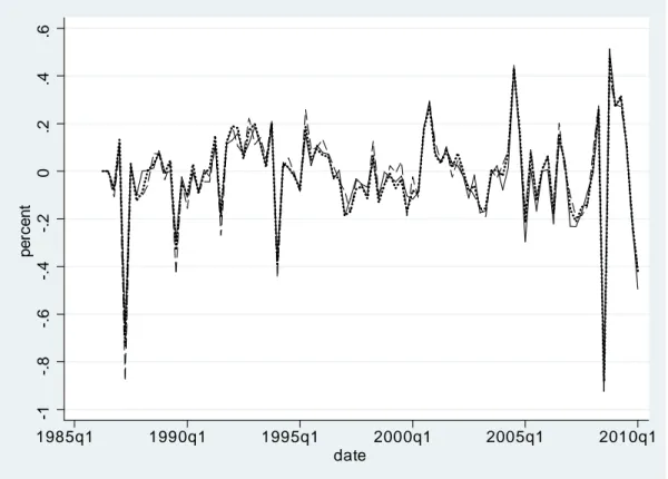
(24) The observable macroeconomic controls included are all signi…cant, suggesting that their omission would bias our analysis. As in Berrospide and Edge (2010), a higher volatility in stock markets tends to imply a lower capital ratio, which may re‡ect higher losses in times of stress. An expected rise in GDP growth is associated with a decrease in capital ratios, which hints at a procyclical behavior of bank leverage. Meanwhile, expected policy rate hikes over the following year are associated with an increase in the current capital ratio, which suggests that this variable can be seen as a "risk factor" impinging on the expected pro…tability of assets. Finally, at least one of the lagged common shocks summarizing the perceived state of the economy emerges as signi…cant, but at the expense of the expected GDP growth regressor, suggesting that this estimated structural macro shock accounts for a large proportion of aggregate GDP ‡uctuations.. 5.3. Aggregate measure of bank capital ratio shocks. Figure 2 shows the aggregate series of capital ratios shocks we obtain for the US banking system. The series has a mean close to zero and a standard deviation of 0.2 percentage points. According to our measure, the largest negative shocks occurred in the second quarter of 1987, the third quarter of 1989, the …rst quarter of 1994, the …rst quarter of 2005, and then, during the last recession, in the …rst semester of 2007 as well as, in the aftermath of the Lehman failure, the third quarter of 2008. Large positive shocks to bank capital ratios occured at the end of 2000, just at the onset of the recession triggered by the burst of the dotcom bubble, and also in the third quarter of 2004 and, last but not least, in early 2009, possibly as a consequence of the TARP program and the ensuing forced recapitalization of US banks during 2009. Note that the panel regression (5) assumes that all banks react in a homogenous way to bank characteristics, as is commonly assumed, but also to the macro shocks. t.. This. last assumption may seem at odds with the …ndings of Buch, Eickmeier and Prieto (2010), who analyze the transmission of macroeconomic shocks to bank risk taking (measured as the share of non-performing loans) and loan growth for the US, using disaggregated information for a large panel of US commercial banks within a FAVAR model. They notably point to heterogenous responses to expansionary monetary and house price shocks, as small banks extend more loans and more capitalized banks tend to make more risky investments (as can be gauged, with the bene…t of hindsight, by looking at the change in bad loans over a horizon of one year). However, it is fair to note that they consider a much more heterogenous population of some 1500 commercial banks with assets larger than $25 million, whereas we. 21.

(25) focus on a contained sample of some 100 large bank holding companies with assets larger than $3 billion, so that the potential for heterogenous behaviour at the bank level is a priori less in our case. Nevertheless, in order to check that our estimated macro shock to bank capital ratio is immune from the possible consequences of such heterogeneity, we restimated equation (5) on di¤erent sub-samples of banks, taking into account only the 25 or 50 largest institutions. As regression coe¢ cients (not shown here for brevity) are not really a¤ected (also less precisely estimated), we …nd con…rmation of the homogeneity assumption. Importantly for our purpose, Figure 3 shows that the estimated aggregate capital ratio shock series also remains broadly unchanged when we restrict the sample to a smaller number of institutions. Giving an economic interpretation to the sign of our aggregate shock series is not straightforward. Indeed, following a positive shock, a bank can increase its capital ratio by only increasing its capital, only decreasing its assets, increasing its capital more than it in‡ates its assets or decreasing its assets by more than its capital shrinks. In other words de-leveraging may be associated with either an expansion or a reduction in a bank’s balance sheet. Mutatis mutandis, the same applies for a negative shock to bank capital ratios. To guide intuition, it may help to look at correlations between asset growth, equity growth and changes in the capital ratios at the individual level. Table 4 shows how the sign of shocks to the ratio relates to the sign of changes in its numerator (equity) and denominator (assets) at bank level within our sample. Note that roughly half of the capital ratio shocks in our sample are positive, which is consistent with the assumption that E("i;t ) = 0 in the panel regression. Looking at positive (i.e. deleveraging) shocks, most if not all of them (94%) are associated with stable or increasing equity, while about half of them are associated with increasing assets. In contrast, some 86% of negative ratio (i.e. leveraging) shocks tend to go in synch with increasing assets, while the equity base goes up in only two thirds of cases. From this we may guess that negative ratio shocks should have rather expansionary e¤ects on the economy. The sign of the aggregate consequences of positive ratio shocks remains, however, unsettled at this stage and should be expected to depend on the size distribution of shocked banks at each point in time.. 5.4. Validating the factor structure of macro series. In practice, having obtained series of realizations of the three real and nominal macro shocks stacked in. t;. as well as of the bank capital ratio shock "t , we get estimates of the. parameters in equation (6) by using simple OLS regressions. Since it appears that usual. 22.

(26) information criteria are not very conclusive about the optimal number of lags to include in each polynomial, we try to keep the model as parsimonious as possible, while allowing for a su¢ ciently rich dynamic of the response of individual variables to the aggregate capital ratio shock. We thus choose one lag for the lagged dependent variable, one lag for the nonbanking macro shocks and four lags for the capital ratio shock as our baseline speci…cation. We nevertheless checked that allowing for a richer lag structure (up to four lags for each polynomial) does not qualitatively a¤ect our conclusions. A comparison of IRFs for di¤erent sets of lags of the polyomials in equation (6) is presented in Figures 6-7. The …gures con…rm that our main results are quite robust to reasonable changes to lag selection. An important underlying assumption of our approach is that the series in X have a factor structure and that the dynamic factors extracted from X also span the ancillary variables in Y . To check this, we conduct Wald tests of joint signi…cance of the coe¢ cients in the FADL regressions of individual macro series, as well as tests of the joint signi…cance of the parameters associated with the contemporaneous and lagged bank capital ratio shock only. Table 5 presents the results, together with the share of the variance of each macro series that is explained by all regressors vs the capital ratio shock alone. The tests …rst con…rm that our shock series indeed span all the real and nominal macro series stacked in X as well as most of the banking indicators in Y , with the exception of the growth of real estate loans. Interestingly, the null that capital ratio shocks do not matter for explaining macro series is rejected (at the 10% level) for several key activity variables, notably GDP, investment, industrial production, the consumption of non-durables and housing starts, as well as for the corporate spread. The aggregate capital ratio shock also turns out to be a signi…cant determinant of most credit and banking indicators, with the exception of the growth of deposits and of real estate loans, as well as interest rates on personal and new car loans. It is important to note that this …nding is not as such inconsistent with the fact that the capital ratio shock is by construction orthogonal to the contemporaneous common macro shocks driving Xt . Indeed, the capital ratio shock may …rst drive the idiosyncratic component of some of the macro series Xi;t (the ut term in equation 1). Besides, lags of the capital ratio shock may not be orthogonal with the common shocks in. t.. Finally, note. that the factor structure also explains a large share of the variance of some key banking indicators, above 80% for the growth of C&I loans and bank credit rates, although these indicators were not part of the training sample used to extract the non-banking macro shocks. Overall, the results presented in Table 5 suggest that it indeed makes sense to look at. 23.

(27) the IRFs of key macroeconomic and credit indicators to the aggregate capital ratio shock.. 6. Assessing the macroeconomic e¤ects of shocks to the leverage of large banks. Figure 4 presents the response of a selection of macro variables of interest in Xt to a positive bank capital ratio shock of one standard deviation (i.e. about 0.2 percentage points), together with bootstrapped con…dence intervals at the 70% level.20 First, we …nd a large and signi…cant contractionary e¤ect on GDP of this unexpected reduction in the leverage of large banks, with the components of aggregate demand that are a priori most sensitive to the availability of credit showing the largest reaction on impact. Indeed, total productive investment decreases by some 2 percentage points on impact, and slightly more in the second quarter after the shock. Similarly, consumption of durables drops immediately by some 1.5 percentage points, but the e¤ect is short-lived and vanishes after one quarter. Also, consumption of non-durables and total consumption contract with a lag during a couple of quarters after the shock. The responses obtained for interest rates show that, while monetary policy does not seem to react to the bank capital ratio shock itself, the central bank will lower the short term rate by some 50 basis points two quarters after the shock to counteract its recessionary consequences. This persistent decrease in the policy rate is in turn re‡ected in lower risk-free interest rates along the whole yield curve. Finally, a deleveraging shock to bank capital ratios leads to an immediate (although short-lived) increase in the Baa corporate spread. Interestingly, this result echoes the evidence presented by Gilchrist and Zakrajsek (2012) regarding the link between their measure of the excess corporate bond premium - the premium required by corporate bond investors beyond the compensation for the measured default risk of …rms - and the capacity of major …nancial institutions to take risk on their balance sheet, depending in turn on their capital structure. They notably …nd that a deterioration in the pro…tability of broker-dealers leads to rise in their CDS spreads, a good measure of the perceived default risk of these …nancial intermediaries, and an associated rise in the excess corporate bond premium, re‡ecting their reluctance to take on additional risk. As Gilchrist and Zakrajsek also provide evidence that this premium embedded in corporate spreads, and to some extent the total corporate spread itself, are good predictors of future economic activity, this suggests that the consequences of bank leverage 20 Note that the response functions are presented in levels for the sake of clarity, which means that they show the cumulated e¤ects of the capital ratio shock on the growth rates or changes of individual variables whenever the series are non-stationary (like e.g. GDP).. 24.

(28) shocks for the excess corporate bond premium could provide a channel for the transmission of these shocks to activity, beyond the direct e¤ect on lending. Figure 5 in turn presents the responses of the credit and banking indicators stacked in Y , which we do not take into account when extracting the real and nominal shock series from the general macro dataset. Note that, again, none of these IRFs are constrained. Most interestingly, we …nd a large, signi…cant, immediate and persistent decrease in most measures of aggregate credit considered, with the weakest response for consumer credit. Credit to …rms (C&I loans and loans & leases) contracts more than credit to households for housing purposes, by some 2.5% on impact and 10% over the …rst year. Overall, a positive shock to bank capital ratios (i.e. a negative aggregate bank leverage shock) triggers a large and persistent fall in total bank credit and total bank assets over at least six quarters. Total commercial bank credit drops by 2% on impact and about 6% over the following year, the magnitude being similar for bank assets. Last but not least, we …nd that the deleveraging shock implies a signi…cant rise in the spreads between some bank credit rates and monetary policy rates. The increase is notably large and persistent for interest rates on small loans to …rms. The combination of decreasing loan volumes and increasing loan rates suggests that our estimated bank capital ratio shock does identify properly a negative credit supply shock. This is all the more noteworthy that we do not need to impose any sign restrictions to identify this shock. The last two panels at the bottom of Figure 5 show the reaction of two other indicators used in related studies: the index of tightening of credit conditions according to the Loan O¢ cer Survey, and the aggregate measure of the leverage of all US commercial banks as computed in the Flow of funds.21 Credit standards do not seem to tighten following a positive shock to bank capital ratios, which suggests that, at least over our sample period, credit standards were not primarily tightened because of capital constraints on the side of banks.22 This tends to be con…rmed by the almost zero correlation we observe between our capital ratio shock and the aggreate bank lending standard shock provided by Basset et al. 21. Due to a shorter available time series, the IRF for these last two variables are estimated over the period from 1992 to 2010. 22 This may hold in aggregate, although some banks may indeed have tigntened standards and cut lending as a consequence of scarce capital, and in particular most recently in anticipation of more stringent Basel 3 capital requirements. In a recent paper, Basset and Covas (2012) use banks’ own assessments of their capital adequacy as reported to the Fed’s Survey on lending standards to study the link between capital adequacy and lending over the period 1996-2010.They …nd reduced loan growth at banks that tighten lending standards as a result of concerns about their current or future capital position relative to banks that do not report being capital constrained.. 25.