Dynamic Modeling and Validation of Radiant Ceiling Systems Coupled to its Environment

(1)

3123

, Page 1

International High Performance Buildings Conference at Purdue, July 12-15, 2010

Dynamic Modeling and Validation of Radiant Ceiling Systems Coupled to its

Environment

Néstor FONSECA

1

_{*, Cristian CUEVAS}

2

_,

_{Vincent LEMORT}

3 1

Universidad Tecnológica de Pereira, Facultad de Ingeniería Mecánica,

Pereira, Colombia, Phone: 57-6_3137124, E-mail: nfonseca@utp.edu.co

2

_{Universidad de Concepción, Facultad de Ingeniería Mecánica, Chile}

Concepcion, Chile, E-mail: crcuevas@udec.cl

3

_{University of Liège Belgium. Thermodynamics Laboratory,}

Liege, Belgium, E-mail: Vincent.Lemort@ulg.ac.be

* Corresponding Author

ABSTRACT

This paper presents the results of a study performed in order to develop a dynamic model of radiant ceiling panels in heating or cooling modes coupled to its environment (fenestration, walls, internal loads and ventilation system). The model considers the radiant panels as a dynamic-state finned heat exchanger connected to a detailed lumped dynamic model of the building (R-C network). The behavior of the radiant ceiling system and the interactions with its environment has been experimentally and numerically evaluated. Using as inputs the radiant ceiling and room dimensions, material properties and the transient measurements of air temperature at the adjacent zones, supply air and water temperatures and mass flow rates, the model allows for the estimation of the water exhaust temperature, radiant ceiling average surface temperature, resultant and dry air room temperatures, radiant ceiling power and internal surface temperatures of the room in order to compare with measurements taken during the commissioning process. Two dynamic tests in heating and cooling modes are used to validate the model

1. INTRODUCTION

The analysis of the radiant ceiling system becomes a complex process considering that its behavior must be studied by coupling it with the corresponding structure of the building (facade, walls, internal loads and ventilation system), climate and functioning conditions. This is due to that the resultant temperature in a space is not only depending on the air temperature, but also on the transient variation of the surface temperatures in the conditioned space (Fonseca

et al., 2009). A few computer models currently available were developed specially as design tools for radiant

cooling systems and usually as stand-alone programs to evaluate their performances. In general, these models cannot be used to determine the global behaviour of radiant ceiling systems (cooling and heating) in any conditions other than the specific design conditions and without considering for example the effect of the fenestration and ventilation systems or ceiling perforation effects.

The model developed by Kilkis et al. (1995) proposes a design procedure for radiant cooling systems that assumes steady-state conditions where the radiant heat exchange with the facade and walls is simplified as well as in most of the related literature (ASHRAE, 2004; Jae-Weon and Mumma, 2004). The usual practice (Hauser et al., 2000 ) is to connect a model of cooled or heated ceiling with TRNSYS (Klein et. al., 2009) modules for the other room surfaces. TRANSYS model is based on the German standard DIN 4715-1(1993) for the chilled ceiling panels; therefore additional parameters to define the performance in this type of test conditions are needed. However, as the aim of this kind of tests is only to compare the performance of different types of cooling ceiling systems, a homogeneous load distribution is considered without the influences of the ventilation system and/or the facade asymmetry effect (Kochendörfer, 1996 ).

In the EnergyPlus program (2008), the radiant ceiling is then simplified using these assumptions and the effectiveness-NTU method. Consequently, none of the large building energy programs available publicly (TRNSYS, EnergyPlus) has the capability to simulate buildings cooling or heating by radiant ceiling systems with the required detailed level. In the first part of this study (Fonseca et al., 2009), the results of an experimental analysis of radiant

(2)

3123

, Page 2

ceiling systems in heating or cooling mode coupled to its environment is presented. In this part, a separate dynamic model simulates the specifics of radiant cooling systems performance but integrated with its environment, the resultant temperature is therefore calculated as a comfort parameter for design proposes and especially for commissioning processes (Fonseca et al., 2009b).

2. MATHEMATICAL MODEL DESCRIPTION

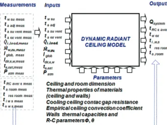
The dynamic model developed in this study basically considers the heat exchange between a room and the adjacent zones. The dynamic thermal balances in dry regime of the active radiant ceiling, room and ceiling void, the external and internal walls thermal balances (including a possible inactive ceiling zone) as well as ceiling and floor slabs are considered. The window behavior is modeled assuming steady-state condition, considering the low thermal inertia of the fenestration system. The cooling ceiling model can be characterized by the inputs, outputs and parameters shown in Figure 1.

Figure 1: Definition of the cooling ceiling model inputs outputs and parameters

2.1 The radiant ceiling model

According to the systems used in this study, two typical individual elements (for six different configurations) of radiant ceiling can be chosen as shown in Fonseca et al. (2009a; 2009b). The radiant ceiling can be therefore considered as a fin where only the dry regime is considered. The thermal balance of this sub-system considers the convective heat transfer on the water side (in transition or turbulent flow as the main design conditions), conduction through the tube shell and union system (tube-ceiling surface) and convective and radiation heat transfers from the tube external surface and ceiling surface to the ceiling cavity and the room. In case of the conductive thermal resistance through plaster layers, two-dimensional steady-state conduction heat transfer is assumed (Rao and Rahmman, 2006; Antonopoulos et al., 1997). In dynamic state, the total thermal power extracted from the zone by water (

Q&

_total) in cooling mode can be calculated from the dynamic water (Eq. 1) and radiant ceiling (Eq. 2) thermal balances as: cavity t RC total w

Q

U

&

=

&

−

&

−

&

, [W] (1)

RC load i room RC cavity RC RC RC

Q

U

&

=

&

−

&

,

−

&

,

−

&

, , [W] (2)

And

∫

=

Δ

2 1

.

τ τ

U

d

τ

U

_w

&

_w [J] (3)

∫

=

Δ

2 1

.

τ τ

U

d

τ

U

_RC

&

_RC [J] (4) [J] (5) [J] (6)

(3)

3123

, Page 3

International High Performance Buildings Conference at Purdue, July 12-15, 2010 where

tw,ave,1 is the initial water average temperature [°C]

tRC,ave,1 is the initial radiant ceiling average temperature [°C] RC

Q&

is the total thermal energy extracted by the radiant ceiling panel, [W]. cavity

t

Q

&

, is the heat flow rate through the tube external surface from the ceiling cavity, [W].

cavity RC

Q

&

, is the heat flow (convection + radiation) coming from the ceiling cavity, [W].

room RC

Q

&

_, is the heat flow (convection + radiation) coming from the room, [W].

RC r load i

Q

&

, ,, is the radiative fraction of the room internal thermal load on the radiant ceiling, [W].

w

C

is the thermal mass of the water into the active radiant ceiling, [J K-1_] RC

C

is the global radiant ceiling thermal mass (tubes, union system and metallic plates) , [J K-1_]

Considering the constant tube surface temperature, the water average temperature is estimated form the log-mean temperature difference for each block of panels connected in series by:

tt – tw;av e tt – tw;su = exp – π Di · h_w · Lt 2 Mw Np · cp;w [°C] (7)

The theoretical approach used in steady-state analysis (Fonseca et al., 2009a) for the fin effectiveness and panel perforations influence are used here as the base of the dynamic modeling.

2.2 Thermal zone model

Two zones are considered in this global model: the room and the ceiling void (Fonseca et al., 2009b). The dynamic behavior of each zone is modeled by an air thermal capacity. The thermal balance of the room is given from equations 8 to 11 according to methodology presented in (Fonseca et al., 2009b).

s i conv floor w i s i conv bottom w i s i conv right w i s i conv left w i s i conv RC inac s i conv RC a

Q

U

&

=

&

_, _,_,

+

&

_, _, _,_,

+

&

_, _, _, _,_,

+

&

_, _, _, _,_,

+

&

_, _, _, _,_,

+

&

_, _, _, _,_,

ven conv load i s i conv win s i conv w e

Q

&

+

&

+

&

+

&

+

, , ,, , ,, , , [W] (8)

∫

=

Δ

2 1

.

τ τ

U

d

τ

U

_a

&

_a [J] (9) [J] (10) room a a p c i f a

F

c

V

C

=

_,_,

.

_,

.

ρ

.

[J K-1_] (11)

The thermal balance considers the convective heat flow rate on each surface in contact with the air room, including the possibility of an inactive ceiling surface. The air capacity is corrected by a hypothetical factor (

F

_f,_i,_c), supposed to consider the capacity of all the internal surfaces and equipment (Walls and furniture) inside the room.

The

Q

&

_i,_load,_conv value is the convective portion of the internal thermal load and

Q&

ven is the sensible contribution of

the mechanical ventilation system. The same method is applied to the ceiling void. The convective heat transfer coefficients on the internal side of the room walls are calculated from Churchill and Chu correlations. For the floor surface the Mc Adams correlations are used (Incropera and DeWitt, 1996). The convective heat exchange on the radiant ceiling surface (active or inactive) is a more complex process, considering the combined effects of ventilation, ceiling perforations, internal thermal loads, facade and radiant ceiling operation. The number of configurations and possible combinations of these elements in modern buildings avoid describing completely the phenomenon with a correlative method. Existing correlations were developed from experimental measurements in specific conditions of ventilation and internal thermal loads (Alamdari and Hammond, 1983; Spitler et al., 1997;Awbi and Hatton 2000). According to ASHRAE (2004), only natural convection (NC) should be considered

(4)

3123

, Page 4

on the radiant ceiling surface. However, among others to ensure that the radiant ceiling system in cooling mode is operating only in dry regime, moisture has usually to be removed from the room through a mechanical ventilation system which generates some air movement. Forced convection (FC) is negligible if (Gr/Re2_{) » 1. Hence the} combined free and forced (or mixed) convection regime is generally one for which (Gr/Re2_{) ≈ 1. In this study, the} current order of magnitude found for (Gr/Re2_{) is between 0.9 and 0.68. Therefore to combine the effects of natural} and forced convection on ceiling surface the Yuge method (1960) is used.

o NC room RC comb room RC NC room RC FC room RC NC room RC comb room RC NC room RC FC room RC FC room RC comb room RC NC room RC FC room RC comb room RC Nus Nus Nus Nus For G Nus Nus Nus Nus For R Nus Nus Nus Nus For Nus Δ + = = Δ + = < Δ + = > = , , , , , , , , , , , , , , , , , , , , , , , , , , ....; : ....; : ....; : [-] (12) With: [-] (13) [-] (14)

The effect of buoyancy on heat transfer in a forced flow is strongly influenced by the direction of the buoyancy force relative to that of the flow. For a perpendicular direction (transverse flow) caused by ventilation system, buoyancy acts to enhance the rate of heat transfer associated with pure forced convection. The Yuge method was developed originally for mixed convection on a sphere in transverse flow. For a flat plate in transverse flow, the adaptation of coefficients m, n and Δ0 performed in this study gives the following results:

NC room cc NC room

Nus

m

, , ; ,

1 .

0

1

011 .

0

7 +

+

=

[-] (15) NC room cc

Nus

n

, ,

2 .

0

2

993 .

0 +

=

[-] (16) NC room cc o

=

0 .

257 *

Nus

, ,

Δ

[-] (17)

For a ventilated radiant ceiling, the Reynolds number close to the diffusers is usually around 25000 and the Eq. 18 can be used for forced convection (FC) on a horizontal plate in parallel and laminar flow (Incropera and DeWitt, 1996). 3 / 1 2 / 1 , ,roomFC

0 .

664 Re

L

Pr

cc

Nus

=

[-] (18) With:

ν

FC RC L

L

u

_,

Re

=

∞ [-] (19)

The air velocity on the cooling ceiling (u∞) and the characteristic length in forced convection (LRC,FC : distance of jet detachment) are defined from diffuser manufacturer’s catalogue. Finally, the mixed local heat transfer coefficient is given from Eq. 20.

comb room RC RC c a conv room RC

Nu

L

k

h

_, _, , , ,

=

[-] (20)

The characteristic length of mixed convection (Lc,RC) has to be experimentally identified, this is due to the fact that in modern buildings there are too many configurations and possible combinations of ventilation systems, thermal load types and distributions as well as the facade effect.

2.3 Wall model

A two-port R-C network model is used to simulate each surrounding wall (floor and ceiling slabs, partition walls). The parameters of this wall R-C network are adjusted through a frequency characteristic analysis (Bertagnolio, 2008).The (convective) thermal balance on the internal node of the external wall model can be expressed as follows:

(5)

3123

, Page 5

w e in w e out w e

Q

U

&

_,

=

&

_, _,

−

&

_, _, [W] (21)

∫

=

Δ

2 1

.

, , τ τ

U

d

τ

U

ew

&

ew [J] (22) [J] (23) w e p w e w e w e

m

c

C

,

=

φ

,

.

,

.

,, [J K -1 ] (24)

The balance of the external side of the wall gives:

sky w e sun w e s e conv w e out w e

Q

&

, ,

=

&

, , , ,

+

&

, ,

−

&

, , [W] (25)

Where: s e conv w e s e w e f adj a out w e

R

t

Q

, , , , , , , , , , ,

−

=

&

[W] (26) s e w e w e s e conv w e

h

A

R

, , , , , , , ,

.

1 =

[K W-1_]₍₂₇₎ s e conv w e out w e w e c s e w e out w e

R

t

Q

, , , , , , , , , , , , ,

₋

−

=

&

[W] (28) [K W-1_]₍₂₉₎ w e total w e

AU

R

, , ,

1 =

[K W-1_]₍₃₀₎

The values

θ

_e,_w and

φ

_e,_w are the accessibility and proportion parameters respectively (R-C network) of the considered wall. They are obtained using the methodology proposed by Bertagnolio (2008).

The balance of the internal side of the external wall gives:

0

, , , , , , , , , , ,

,win

+

ewiloadrad

+

ewrad

−

ewconvis

=

e

Q

&

[W] (31)

With: total s i room w e w i rad rad load i rad load i w e

A

Q

, , , , , , , , , , , ,

&

.φ

.

&

=

[W] (32) Where RC rad w i rad,,

1 φ

,

φ

=

−

[-] (33)

The coefficient

φ

_{rad ,}_RCis the radiative fraction of the internal thermal load or gain to the radiant ceiling (from the view factors). And:

win sun rad load i load i rad load i

Q

&

, ,

=

&

,

.

φ

, ,

+

&

, [W] (34)

With conv load i rad load i, ,

1 φ

, ,

φ

=

−

[-] (35)

The coefficient

φ

_i_,_load_,_conv is the convective fraction of the internal thermal load or gain. The sun heat radiation though the window is considered here as an internal thermal load and distributed on each internal wall surface. Finally, the conductive heat flux through the wall can be defined as follows:

s i conv w e in w e s i w e w e c in w e

R

t

Q

, , , , , , , , , , , , ,

₋

−

=

&

[W] (36) total w e w e in w e

R

_, _,

=

θ

_,

.

_, _, [K W-1_]₍₃₇₎

(6)

3123

, Page 6

For the internal walls, the methodology is almost the same, obviously without the effect of the sun and infrared radiation with the sky considered in the external wall surface. On the outdoor side, in the case of external walls, solar gains and sky infrared losses are taken into account and injected or taken out of the surface node of the wall. The equation used to compute solar gains and infrared losses through the external wall and window are taken from (Bertagnolio, 2008). Radiation heat exchanges between walls are computed by means of the radiosity method. The view factors can be calculated for the surfaces considered (15 surfaces). This method supposes that the surface temperatures are known.

2.4 Room-resultant temperature

The resultant temperature can be estimated in a detailed way from calculated surface temperatures and the corresponding view factors between the person and surfaces. In this case the mean radiant temperature (MRT) viewed by a sphere of 60 cm of diameter (representing a seat person) placed in different positions inside the room is calculated according to:

[K] (38)

The view factors (F0,j) can be calculated for the surfaces and the sphere position inside the room (24 surfaces). The resultant temperature can be therefore calculated as:

[°C] (39)

This calculus can be further compared to the measure of globe temperature at the same place to evaluate the comfort conditions in different places inside the room, in the frame of the design or commissioning process. The resultant temperature and PMV and PPD indices are calculated by means of the classical Fanger’s method and used here as a comfort variable in order to evaluate the global performance of the system.

3. DYNAMIC MODEL VALIDATION

The validation process is performed using the test bench described in with the copper tube radiant ceilings in cooling and heating mode. As an example, the model validation is presented here in heating mode. The contact thermal resistance and heat transfer coefficient of this type of radiant ceiling are obtained in steady state conditions from experimental test (Fonseca et al., 2009a) and used in the dynamic model as parameters. The modifications considered here are: the distance and velocity of the jet detachment considering that they are defined from diffuser manufacturer’s catalogue for the specific diffuser model (this parameters as well as the R-C network parameters are used to adjust the model as shown in Figure 1). The model outputs are compared directly with measurements performed during the regulation test.

For heating mode validation,the test duration is 9:30 hours. The main objective is to simulate the heating during the first hours in the morning, after a night cooling, without ventilation and without lighting.

(7)

3123

, Page 7

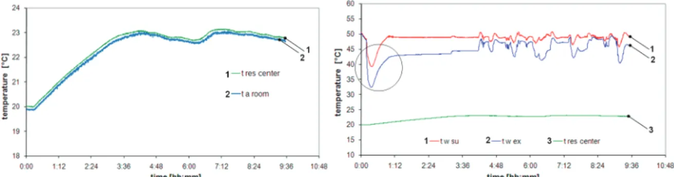
In Figure 2 (resultant and air temperatures at the center of the office and 75 cm above the floor) is observed that during the test, the air temperature is systematically lower than the resultant temperature. This is due to the radiant ceiling operation (the water temperature is around 49°C) and a limited convective effect in heating mode.

The water temperature measurements are shown in Figure 2. The initial perturbation is due to the fact that water exhaust of each panel block is mixed into the collector with the water previously stored in the system (panels and conduits) as a consequence of the by-pass effect.

In heating mode, only six panels placed close to the facade are operating. They are connected in three blocks, each one with two panels connected in series.

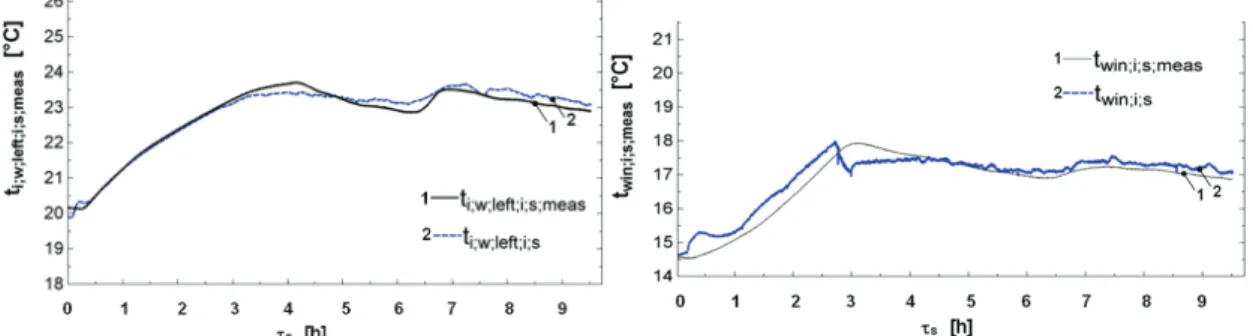
The direct comparison between the model results and measured values of the internal wall and window surface temperatures (at the internal surface) are shown in Figure 3.

Figure 3: Comparison: Measured and calculated temperatures of internal wall and window at the internal surface.

Figure 4: Comparison: Measured and calculated room air and resultant temperatures

The error indicator RMS (root-mean-square) [19] is used to compare the measured and calculated values of the temperatures profiles of n measurements according to:

[°C] (38)

An average error RMS value between simulated and measured values of internal surface temperature of ±0.23K is observed, which is within the measurement uncertainty variation. For air and resultant room temperatures the results are presented in Figure 3 and 4, A RMS error between simulated and measured values of ±0.23K is observed. It is also observed that the calculated value is systematically lower than the measured value. This is due to the fact that the comparison is based on the resultant and air temperatures (ta,room and tres,room) measured in the center of the chamber and 75 cm above the floor, while the model considers homogeneous air conditions. Therefore the temperature stratification induced during the experimental test in heating mode is not considered and can explain an important part of the model error.

(8)

3123

, Page 8

4. CONCLUSIONS

The dynamic model of the radiant ceiling systems and its environment are presented here as a part of the system study in cooling or heating modes. A good agreement is found between simulated and measured values. The results show that the average difference between simulated and measured air and surfaces temperatures is lower than ±0.5 K. However the simulated water exhaust temperature does not follow its dynamic behavior. This is due to model assumptions and the particularities of hydraulic circuits implemented experimentally (more complex than the real case in a building). The air and surfaces temperatures calculated as model outputs consider homogeneity conditions inside the room. The air stratification experimentally induced is not considered in the model and can explain therefore part of the model error. The dynamic model permits to support a global operation testing procedure of the system in the frame of commissioning procedure aiming at the verification of the radiant ceiling behavior coupled to the building, internal thermal loads, fenestration and ventilation systems and evaluation of the comfort conditions of the occupants. In this modeling the resultant temperature is calculated as a comfort indicator, as it depends strongly on the transient variation of the surface temperatures in the room. A dynamic simulation of the whole system must be included in the Functional Performance Testing (FPT) of this system in commissioning process.

REFERENCES

Alamdari, F., Hammond, P., 1983, Improved data correlations for bouyancy-driven convection in rooms, Building

Services Engineering research and Techonology, vol 4. no 3: p.106-112.

Antonopoulos, A., Vrachopoulos, M., Tzivanidis, C., 1997, Experimental and theoretical studies of space cooling using ceiling embeddes piping, Applied Thermal Engineering, vol 17, no. 4: p. 351-36.

ASHRAE HANDBOOK-HVAC Systems and Equipment, 2004, Chapter 6. Atlanta: American Society of Heating, Air-Conditioning and Refrigeration Engineers, Inc.

Awbi, H., Hatton, A., 2000, Mixed convection from heated room surfaces. Energy and Buildings. vol 32: p 153-166. Bertagnolio, S., Masy, G., Lebrun, J., André, P., 2008, Building and HVAC System simulation with the help of an

engineering equation solver, Proceedings of the Simbuild 2008 Conference, Berkeley, USA.

DIN 4715, 1993, Cooling surfaces for rooms; part 1: measuring of the performance with free flow Deutsches Institut Fur Normung E.V. (German National Standard) / 01-Jul-1994 / 13 pages.

EnergyPlus Engineering Document – The Reference to EnergyPlus Calculations, The Ernest Orlando Lawrence Berkeley Laboratory, USA, April 2008.

Fonseca, N., Cuevas, C., Lemort, V., 2009a, Radiant ceiling systems coupled to its environment Part 1: Experimental analysis. In revision. Applied Thermal Engineering

Fonseca, N., Lebrun, J., André, P., 2009b, Experimental study and modeling of cooling ceiling systems using steady- state analysis, International Journal of refrigeration, Article In press.

Hauser, G., Kempkes, C., Olsen, B., 2000, Computer Simulation of hydronic heating/cooling system with embedded pipes, ASHRAE Transaction , vol. 106.

Incropera, F., DeWitt, D., 1996, Fundamentals of Heat and Mass Transfer. Fourth Edition. School of Mechanical Engineering Purdue University.

Jae-Weon, J., Mumma, S., 2004, Simplified cooling capacity estimation model for top insulated metal ceiling radiant cooling panels, Applied Thermal Engineering. vol.24: p. 2055-2072.

Klein, et. al., TRNSYS – A Transient System Simulation Program User Manual, The Solar Energy Laboratory, University of Wisconsin – Madison., 2009.

Kochendörfer, 1996, Standard testing of cooling panels and their use in system planning, ASHRAE Transactions, 102 (1): p. 651-658.

Kilkis, B., 1995, Coolp: A computed program for the design and analysis of ceiling cooling panels, ASHRAE

Transaction: Symposia. SD 95-4-4: p. 705-710.

Rao, C, Rahmman, M., 2006, Transient conjugate heat transfer model for circular tubes inside a rectangular substrate, Journal of Thermophysics and Heat Transfer, vol 20: p.122-134.

Spitler, J., Pedersen, C., Fisher, D., Interior convective heat transfer in buildings with large ventilative flow rates. ASHRAE Transaction 97 (1): p. 505-515.

Yuge, T., 1960, Experiments on heat transfer from spheres including mixed natural and forced convection, Trans.