Essays in macro finance and monetary economics

Essays in Macro Finance and Monetary Economics

par

Modeste Yirbèhogré Somé

Département de sciences économiques

Faculté des arts et sciences

Thèse présentée à la Faculté des études supérieures

en vue de l’obtention du grade de Philosophiæ Doctor (Ph.D.)

en sciences économiques

Janvier 2015

Cette thèse intitulée :

Essays in Macro Finance and Monetary Economics

présentée par :

Modeste Yirbèhogré Somé

a été évaluée par un jury composé des personnes suivantes :

Benoît Perron

président-rapporteur

Francisco Ruge - Murcia directeur de recherche

Julien Bengui

membre du jury

Steven Ambler

examinateur externe

Michel Delfour

vice-doyen, représentant du doyen de la FAS

Thèse acceptée le 30 Janvier 2015

Remerciements

Je tiens ici à remercier d’abord mon directeur de recherche Francisco Ruge -Murcia qui m’a toujours soutenu tout au long de mon parcours. Il a été d’une patience incroyable à mon égard et une grande partie de cet aboutissement a été grâce à lui. Je le remercie sincèrement du fond de mon cœur pour les connaissances qu’il a bien voulu partagées avec moi.

Je remercie également mes deux coauteurs d’Afrique du Sud le Professeur Eric Schaling et le Professeur Alain Kabundi qui ont bien voulu accepter collaborer dans un chapitre de ma thèse.

Ensuite, un grand merci à l’ensemble des professeurs du département d’économie de l’Université de Montréal qui ont toujours été à la disposition des étudiants. Je suis reconnaissant particulièrement envers Rui Castro, Alesandro Riboni, Marine Carrasco, Yves Sprumont, William McCausland, Gerard Gaudet, Marc Henry, Bénoit Perron, André Martens, Jean - Marie Dufour qui m’ont dispensé les enseignements tout au long du programme.

Je n’oublierai pas de remercier mes amis et collègues du programme qui ont eu des soutiens divers et de tout genre à mon égard tout au long du programme. Très spécialement je remercie Agbaglah Messan, mon ami et frère avec qui j’ai vécu et partagé de moments agréables pendant toutes ces années. Je remercie également Blache Paul, Rachidi Kotchoni, Doko Firmin, Constant Lonkeng, et tous les autres amis du département qui ont toujours été à mes côtés dans les bons comme dans les di¢ ciles moments. A mes collègues, Ulrich, Selma, Walter, Firmin, Rachidi avec qui j’ai partagé le bureau de façon conviviale, je vous dis grand merci. Comment ne pas remercier mes amis de Montréal qui ne sont pas du département ? Très spé-cialement je tiens à remercier David Zongo, Cedric Okou, Serge Bationo, Abraham Bayala, Kenneth et tous les autres amis qui ont en fait été ma famille au Canada. Je remercie également mon amie et con…dente de tout temps Mme Lonkeng Judith qui m’a toujours apporté son soutien. Je remercie Carlene Sandra, cette merveilleuse et inspirante amie qui était toujours là pour me remonter le moral.

parents au monde. Ils se sont toujours sacri…és pour moi dès le bas âge jusqu’à maintenant. Ma tante Marie Bernard, mon oncle Bénoit, mes cousins Davy, Sonia et Adéline, m’ont toujours soutenu et je les remercie in…niment pour cette bonté.

Finalement je remercie le Département de sciences économiques de l’Université de Montréal et le Centre de Recherche Interuniversitaire en Économie Quantitative (CIREQ) qui ont été en fait les acteurs principaux qui m’ont soutenu …nancièrement.

Résumé

Les questions abordées dans les deux premiers articles de ma thèse cherchent à comprendre les facteurs économiques qui a¤ectent la structure à terme des taux d’in-térêt et la prime de risque. Je construis des modèles non linéaires d’équilibre général en y intégrant des obligations de di¤érentes échéances. Spéci…quement, le premier article a pour objectif de comprendre la relation entre les facteurs macroéconomiques et le niveau de prime de risque dans un cadre Néo-keynésien d’équilibre général avec incertitude. L’incertitude dans le modèle provient de trois sources : les chocs de pro-ductivité, les chocs monétaires et les chocs de préférences. Le modèle comporte deux types de rigidités réelles à savoir la formation des habitudes dans les préférences et les coûts d’ajustement du stock de capital. Le modèle est résolu par la méthode des perturbations à l’ordre deux et calibré à l’économie américaine. Puisque la prime de risque est par nature une compensation pour le risque, l’approximation d’ordre deux implique que la prime de risque est une combinaison linéaire des volatilités des trois chocs. Les résultats montrent qu’avec les paramètres calibrés, les chocs réels (produc-tivité et préférences) jouent un rôle plus important dans la détermination du niveau de la prime de risque relativement aux chocs monétaires. Je montre que contraire-ment aux travaux précédents (dans lesquels le capital de production est …xe), l’e¤et du paramètre de la formation des habitudes sur la prime de risque dépend du degré des coûts d’ajustement du capital. Lorsque les coûts d’ajustement du capital sont élevés au point que le stock de capital est …xe à l’équilibre, une augmentation du paramètre de formation des habitudes entraine une augmentation de la prime de risque. Par contre, lorsque les agents peuvent librement ajuster le stock de capital sans coûts, l’e¤et du paramètre de la formation des habitudes sur la prime de risque est négligeable. Ce résultat s’explique par le fait que lorsque le stock de capital peut être ajusté sans coûts, cela ouvre un canal additionnel de lissage de consommation pour les agents. Par conséquent, l’e¤et de la formation des habitudes sur la prime de risque est amoindri. En outre, les résultats montrent que la façon dont la banque centrale conduit sa politique monétaire a un e¤et sur la prime de risque. Plus la banque centrale est agressive vis-à-vis de l’in‡ation, plus la prime de risque diminue

et vice versa. Cela est due au fait que lorsque la banque centrale combat l’in‡ation cela entraine une baisse de la variance de l’in‡ation. Par suite, la prime de risque due au risque d’in‡ation diminue.

Dans le deuxième article, je fais une extension du premier article en utilisant des préférences récursives de type Epstein –Zin et en permettant aux volatilités condi-tionnelles des chocs de varier avec le temps. L’emploi de ce cadre est motivé par deux raisons. D’abord des études récentes (Doh, 2010, Rudebusch and Swanson, 2012) ont montré que ces préférences sont appropriées pour l’analyse du prix des actifs dans les modèles d’équilibre général. Ensuite, l’hétéroscedasticité est une caractéristique courante des données économiques et …nancières. Cela implique que contrairement au premier article, l’incertitude varie dans le temps. Le cadre dans cet article est donc plus général et plus réaliste que celui du premier article. L’objectif principal de cet article est d’examiner l’impact des chocs de volatilités conditionnelles sur le niveau et la dynamique des taux d’intérêt et de la prime de risque. Puisque la prime de risque est constante a l’approximation d’ordre deux, le modèle est résolu par la méthode des perturbations avec une approximation d’ordre trois. Ainsi on obtient une prime de risque qui varie dans le temps. L’avantage d’introduire des chocs de volatilités condi-tionnelles est que cela induit des variables d’état supplémentaires qui apportent une contribution additionnelle à la dynamique de la prime de risque. Je montre que l’ap-proximation d’ordre trois implique que les primes de risque ont une représentation de type ARCH-M (Autoregressive Conditional Heteroscedasticty in Mean) comme celui introduit par Engle, Lilien et Robins (1987). La di¤érence est que dans ce modèle les paramètres sont structurels et les volatilités sont des volatilités conditionnelles de chocs économiques et non celles des variables elles-mêmes. J’estime les paramètres du modèle par la méthode des moments simulés (SMM) en utilisant des données de l’économie américaine. Les résultats de l’estimation montrent qu’il y a une évidence de volatilité stochastique dans les trois chocs. De plus, la contribution des volati-lités conditionnelles des chocs au niveau et à la dynamique de la prime de risque est signi…cative. En particulier, les e¤ets des volatilités conditionnelles des chocs de productivité et de préférences sont signi…catifs. La volatilité conditionnelle du choc de productivité contribue positivement aux moyennes et aux écart-types des primes de risque. Ces contributions varient avec la maturité des bonds. La volatilité condi-tionnelle du choc de préférences quant à elle contribue négativement aux moyennes et positivement aux variances des primes de risque. Quant au choc de volatilité de la politique monétaire, son impact sur les primes de risque est négligeable.

Le troisième article (coécrit avec Eric Schaling, Alain Kabundi, révisé et resoumis au journal of Economic Modelling) traite de l’hétérogénéité dans la formation des attentes d’in‡ation de divers groupes économiques et de leur impact sur la politique

monétaire en Afrique du sud. La question principale est d’examiner si di¤érents groupes d’agents économiques forment leurs attentes d’in‡ation de la même façon et s’ils perçoivent de la même façon la politique monétaire de la banque centrale (South African Reserve Bank). Ainsi on spéci…e un modèle de prédiction d’in‡ation qui nous permet de tester l’arrimage des attentes d’in‡ation à la bande d’in‡ation cible (3% -6%) de la banque centrale. Les données utilisées sont des données d’enquête réalisée par la banque centrale auprès de trois groupes d’agents : les analystes …nanciers, les …rmes et les syndicats. On exploite donc la structure de panel des données pour tester l’hétérogénéité dans les attentes d’in‡ation et déduire leur perception de la politique monétaire. Les résultats montrent qu’il y a évidence d’hétérogénéité dans la manière dont les di¤érents groupes forment leurs attentes. Les attentes des analystes …nanciers sont arrimées à la bande d’in‡ation cible alors que celles des …rmes et des syndicats ne sont pas arrimées. En e¤et, les …rmes et les syndicats accordent un poids signi…catif à l’in‡ation retardée d’une période et leurs prédictions varient avec l’in‡ation réalisée (retardée). Ce qui dénote un manque de crédibilité parfaite de la banque centrale au vu de ces agents.

Mots-clés : Models d’équilibre général, Structure à terme, Prime de risque, ARCH-M, Attentes d’in‡ation.

Abstract

This thesis consists of three essays in the areas of macro …nance and monetary economics. The …rst two essays deal with the analysis of the term structure of interest rates in dynamic and stochastic general equilibrium (DSGE) models. The third essay explores in‡ation expectations formation across di¤erent economic groups in South Africa.

Interest rates are one channel through which monetary policy a¤ects the real economy. Typically, central banks implement monetary policy by in‡uencing short term interest rates. Theoretically, the interest rate on a long-term bond is the average of expected future short term interest rates over the maturity period, plus a risk premium demanded by the holder of the bond to compensate for the risk involved in holding a longer maturity bond. Therefore, any changes in the target rate of the central bank and the risk premium a¤ect long – term interest rates, such as mortgage rates and interest rates on certain durable goods. It is then important for the central bank to understand the economic factors that a¤ect both components of long - term interest namely the market expectations about the short - term rates and the risk premium. For example, recently in the U.S. economy, between June 2004 and June 2006, the ine¤ectiveness of monetary policy to a¤ect long - term interest rates has been attributed to a decline in risk premium over this period, which has o¤set the e¤ect of the increase in the target rate of the Federal Reserve (Fed). In the implementation of its monetary policy, the central bank can more or less control agents’expectations through transparent communication. However, the risk premium is endogenous and unobservable and therefore can not be fully controlled by the central bank. On the other hand, achieving the goal of prices stability in an in‡ation targeting framework depends on the credibility of the central bank.

In the …rst two essays I explore the economic factors of the term structure of interest rates and risk premiums. I build a non-linear dynamic stochastic general equilibrium (DSGE) models whereby I incorporate a range of bonds with di¤erent maturities. Speci…cally, the goal of the …rst essay is to understand the relationship between macroeconomic factors and the level of risk premium in a New Keynesian

general equilibrium framework. Uncertainty in the model comes from three sources : productivity, monetary policy and, preferences shocks. The model has two types of real rigidities namely habit formation in preferences and adjustment costs in capital stock. The model is solved by perturbation method up to second order and calibrated to the U.S. economy. Since the risk premium is by nature a compensation for risk, the second - order approximation implies that the risk premium is a linear combination of the volatility of the three shocks. Results show that at the calibrated parameters, real shocks (productivity and preferences) play a more important role in determining the level of the risk premium relative to monetary shocks. I show that, contrary to previous work (where production capital is …xed), the e¤ect of habit formation on the risk premium depends on the degree of capital adjustment cost. When capital adjustment costs are so high that the capital stock is …xed in equilibrium, an in-crease in the parameter of habit formation leads to an inin-crease in the risk premium. However, when agents can freely adjust the capital stock without cost, the e¤ect of the habit formation parameter on the risk premium is negligible. This result is explained by the fact that when the capital stock can be adjusted without cost, it opens an additional channel to the agents for consumption smoothing. Therefore, the e¤ect of habit formation on the risk premium is reduced. In addition, the results show that the way the central bank conducts its monetary policy has an e¤ect on the risk premium. The more aggressive the central bank vis-à-vis in‡ation, the lower the risk premium and vice versa. This is due to the fact that when the central bank …ghts against in‡ation it leads to a decrease in the variance of in‡ation. As a result, the risk premium due to in‡ation risk decreases.

In the second essay, I extend the analysis of the …rst essay by using recursive preferences (as those proposed by Epstein - Zin) and by allowing the conditional volatility of the shocks to be time - varying. The use of this framework is motivated by two reasons. First, recent studies (Doh, 2010, Rudebusch and Swanson, 2012) sho-wed that these preferences are appropriate for the analysis of asset prices in general equilibrium models. Second, heteroscedasticity is a prominent feature of economic and …nancial data. This implies that, contrary to the …rst essay, the uncertainty here is time - varying. Thus, the framework in this essay is more general and realistic than in the …rst essay. The main objective of this paper is to examine the impact of uncertainty due to conditional volatility of the shocks on the level and the dy-namics of interest rates and risk premiums. Since the risk premium is constant at second order approximation, the model is solved by the perturbation method with an approximation of order three in order to get a time - varying risk premium. The advantage of introducing shocks conditional volatilities is that , it induces additional state variables that provide an additional contribution to the dynamics of the risk

premium. I show that the risk premiums implied by the third – order approximate solution have an ARCH-M (Autoregressive Conditional Heteroscedasticty in Mean) type representation as that introduced by Engle, Lilien and Robins (1987). The dif-ference is that in this model the parameters are structural and the volatilities are conditional volatility of economic shocks and not those of the variables themselves. I estimate the model parameters by Simulated Method of Moments (SMM) using U.S. data. The estimation results show that there is evidence of stochastic volati-lity in the three shocks. Moreover, the contribution of conditional shocks volativolati-lity to the level and the dynamics of the risk premium is signi…cant. In particular, the e¤ects of the conditional volatility of productivity and preferences shocks are impor-tant. The conditional volatility of the productivity shock contributes positively to the means and standard deviations of risk premiums. These contributions vary with the maturity of the bonds. Conditional volatility of the preferences shock contributes negatively to the averages and positively to the variances of risk premiums. As for the impact of volatility of monetary policy shock, its impact on the risk premium is negligible.

The third article (coauthored with Eric Schaling and Alain Kabundi, revised and resubmitted to the journal of Economic Modelling) deals with heterogeneity in in‡ation expectations of di¤erent economic agents and its impact on monetary policy in South Africa. The main question is to examine whether di¤erent groups of economic agents form their in‡ation expectations in the same way and if they perceive the central bank (South African Reserve Bank) monetary policy in the say way. We specify an in‡ation expectation model that allows us to directly test whether in‡ation expectations are anchored or not to the in‡ation target band (3% - 6%). The data used are in‡ation expectations data from surveys conducted by the central bank. There are three groups of agents : …nancial analysts, businesses and trade unions. We therefore exploits the panel structure of the data to test the heterogeneity in in‡ation expectations and derive their perceived in‡ation targets. Results show that there is evidence of heterogeneity in the way the three groups form their expectations. The expectations of …nancial analysts are well anchored to the central bank target band while those of businesses and trade unions are not. In fact, businesses and trade unions put a higher weight on lagged realized in‡ation in their expectations. This Indicates a lack of full credibility of the central bank.

Keywords : DSGE, Term structure, In‡ation expectations, ARCH-M, Risk pre-mium.

Dédicace ii

Remerciements iii

Résumé v

Abstract viii

Table des matières xv

Liste des …gures xv

Liste des tableaux xv

Introduction 1

1 A General Equilibrium Analysis of the Term Structure of Interest

Rates. 5

1.1 Introduction . . . 5

1.2 The Model . . . 8

1.2.1 Households . . . 9

1.2.2 Firms . . . 11

1.2.3 Monetary Policy Rule and Government . . . 15

1.2.4 Market Clearing and Aggregation . . . 16

1.2.5 Equilibrium . . . 17

1.3 Interest Rates and Risk Premia in DSGE Models . . . 17

1.4 Model Solution . . . 20

1.5 Estimation . . . 22

1.5.1 Data . . . 22

1.5.2 Paramaters Estimation : Simulated Method of Moments (SMM) 22

1.5.3 Calibration . . . 23

1.5.4 Parameters Estimates . . . 24

1.6 Results and Sensitivity Analysis . . . 25

1.6.1 The term structure of interest rates . . . 25

1.6.2 Shocks contribution to risk premium . . . 26

1.6.3 Sensitivty Analysis . . . 28

1.7 Conclusion . . . 30

2 Time - varying Volatility and Risk Premia in General Equilibrium 38 2.1 Introduction . . . 38

2.2 Stylized Facts of Term Structure of Bond Interest Rates . . . 42

2.3 The Model . . . 43

2.3.1 Households . . . 44

2.3.2 Firms . . . 48

2.3.3 Monetary Policy Rule and Government . . . 51

2.3.4 Market Clearing and Aggregation . . . 52

2.3.5 Stationary Equilibrium . . . 52

2.4 Interest Rates and Risk Premia in DSGE Models . . . 54

2.5 Model Solution . . . 56

2.6 Econometric Analysis . . . 59

2.6.1 Data . . . 59

2.6.2 Paramaters Estimation : Simulated Method of Moments (SMM) 59 2.6.3 Calibration . . . 62

2.6.4 Parameters Estimates . . . 62

2.7 Results . . . 64

2.7.1 Implications for the Term Structure . . . 64

2.7.2 Risk Premia and Volatility Shocks . . . 67

2.8 Conclusion . . . 70

3 Monetary Policy and Heterogeneous In‡ation Expectations in South Africa 81 3.1 Introduction . . . 81

3.2 In‡ation and In‡ation Expectations in South Africa : An Overview . 83 3.3 The Model . . . 86

3.4 Econometric and Data Analysis . . . 89

3.4.1 Econometric Analysis . . . 89

3.5 Empirical Results . . . 91

3.5.1 Anchoring of In‡ation Expectations . . . 91

3.5.2 Heterogeneity of In‡ation Expectations . . . 92

3.5.3 Credibility and Implicit In‡ation Targets . . . 93

3.5.4 Expectations Trap ? . . . 95

3.6 Conclusion . . . 97

Conclusion 104 Annexe 113 3.1 Appendices for Chapter 2 . . . 113

3.1.1 Appendix 1 : Unit Root Test . . . 113

3.1.2 Appendix 2 : Model Moments at the SMM Estimates . . . 113

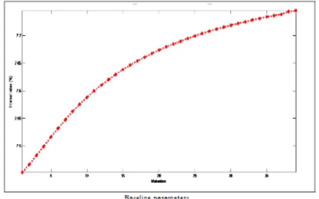
1.1 Average Term Structure of Interest Rates . . . 33

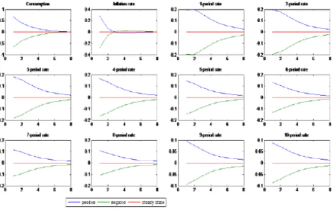
1.2 Impulses Responses to Monetary Policy Shock . . . 34

1.3 Impulses Responses to Productivity Shock . . . 34

1.4 Impulses Responses to Preferences Shock . . . 35

1.5 Shocks Contribution to Risk Premia . . . 35

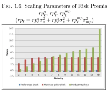
1.6 Scaling Parameters of Risk Premia . . . 36

1.7 The E¤ect of Monetary Policy Action ( ) on Risk Premium (10 - year) 36 1.8 The E¤ect of Habit Formation (b) on Risk Premium (10 - year) . . . 37

1.9 The E¤ect of Consumption Curvature ( c) on Risk Premium (10 - year) 37 2.1 Model Implied Term Structure of Interest Rates . . . 74

2.2 Simulated Series of the Term Structure . . . 75

2.3 Responses to Productivity Level Shock . . . 76

2.4 Responses to Preferences Level Shock . . . 76

2.5 Responses to the Monetary Policy Level Shock . . . 77

2.6 Responses to the Productivity Volatility Shock . . . 77

2.7 Responses to Preferences Volatility Shock . . . 78

2.8 Responses to Policy Volatility Shock . . . 78

2.9 Risk Premium and Conditional Volatility E¤ects Coe¢ cients . . . 79

2.10 Sensitivity Analysis . . . 80

3.1 In‡ation and In‡ation Expectations :Aggregate . . . 102

3.2 In‡ation and In‡ation Expectations per Group . . . 103

3.1 Responses of Macro Variables to shocks . . . 115

3.2 Responses to Monetary Policy Shocks um _{. . . 116}

3.3 Responses of Macro Variables to Volatility Shocks . . . 117

3.4 Responses to Monetary Policy Volatility Shock . . . 117

Liste des tableaux

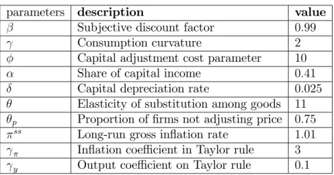
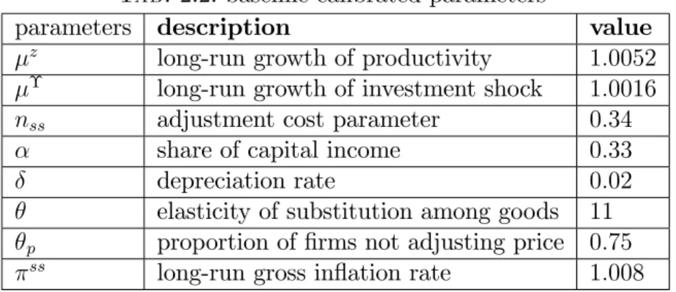
1.1 Baseline Calibrated Parameters . . . 25

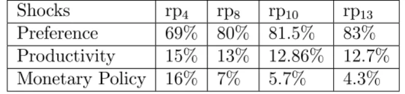
1.2 Shock Contribution to Risk Premia (Baseline Parameters) . . . 27

1.3 Prices of Risk (Baseline Parameters) . . . 28

1.4 Unit Roots Test . . . 31

1.5 SMM Estimation . . . 32

1.6 Model implied term structure statistics, baseline calibrated parameters 32 2.1 Selected Term Structure Statistics :Sample : 1962Q1 2001Q3 . . . . 43

2.2 baseline calibrated parameters . . . 72

2.3 SMM Estimation . . . 73

3.1 StationarityTest of In‡ation and in‡ations expectations . . . 99

3,2 Granger Causality Test . . . 99

3.3 Heterogeneity in Average In‡ation Expectations . . . 100

3.4 Heterogeneity in Slopes and Intercepts . . . 100

3.5 Expectations Formation and Implicit In‡ation Target by Agent . . . . 101

3.6 Optimal in‡ation Regression . . . 101

3.1 Unit Roots Test . . . 113

Introduction Générale

Cette thèse est composée de trois chapitres dans les domaines de la macro …nance et de la macroéconomie monétaire. Les deux premiers chapitres traitent de l’analyse de la structure à terme des taux d’intérêt dans les modèles dynamiques et stochas-tiques d’équilibre général. Quant au troisième chapitre, il traite de la modélisation des attentes d’in‡ation de di¤érents agents dans l’économie Sud-Africaine.

L’un des canaux traditionnels de transmission de la politique monétaire sur l’ac-tivité réelle est celui des taux d’intérêt. En e¤et, typiquement la banque centrale met en œuvre la politique monétaire en in‡uant sur les taux d’intérêt de court terme. Elle relève et abaisse le taux cible du …nancement à un jour, qui est le taux auquel les grandes institutions …nancières se prêtent des fonds au jour le jour. Selon la théorie, le taux d’intérêt sur une obligation à long terme est la moyenne des attentes des taux d’intérêt futurs à court terme entre aujourd’hui et la date d’échéance de l’obli-gation, plus une prime de risque réclamée par le détenteur de l’obligation en guise de compensation pour le risque qu’il court en détenant une obligation de plus longue maturité. Par conséquent, toutes variations des taux cibles de la Banque centrale et de la prime de risque se répercutent sur les taux d’intérêt de plus long terme, tels que les taux d’intérêt sur les prêts hypothécaires et les taux d’intérêt sur certains biens durables. Pour une politique monétaire e¢ cace la banque centrale se doit donc de comprendre les facteurs économiques qui a¤ectent les deux composantes des taux d’intérêt de longs termes à savoir les attentes des agents sur les taux de courts termes et la prime de risque. Par exemple, récemment dans l’économie américaine, entre juin 2004 et juin 2006, l’ine¢ cacité de la politique monétaire à a¤ecter les taux d’intérêt de long terme a été attribuée à une baisse de la prime de risque sur cette période qui a contrebalancé l’e¤et de la hausse du taux cible de la banque centrale américaine (Fed). Dans la mise en œuvre de sa politique monétaire, la banque centrale peut plus ou moins contrôler les attentes des agents par une communication transparente. Cependant la prime de risque est endogène et inobservable et ne peut donc être entièrement contrôler par la banque centrale. En outre, l’atteinte de l’objectif tradi-tionnel de control d’in‡ation des banques centrales dépend des attentes des agents

économiques sur l’in‡ation future.

Les questions abordées dans les deux premiers articles cherchent à comprendre les facteurs économiques qui a¤ectent la structure à terme des taux d’intérêt et la prime de risque. Je construis des modèles non linéaires d’équilibre général en y intégrant des obligations de di¤érentes échéances. Spéci…quement, le premier article a pour objectif de comprendre la relation entre les facteurs macroéconomiques et le niveau de prime de risque dans un cadre Néo-keynésien d’équilibre général avec incertitude. L’incertitude dans le modèle provient de trois sources : les chocs de productivité, les chocs monétaires et les chocs de préférences. Le modèle comporte deux types de rigidités réelles à savoir la formation des habitudes dans les préférences et les couts d’ajustement du stock de capital. Le modèle est résolu par la méthode des perturbations à l’ordre deux et calibré à l’économie américaine. Puisque la prime de risque est par nature une compensation pour le risque, l’approximation d’ordre deux implique que la prime de risque est une combinaison linéaire des volatilités des trois chocs. Les résultats montrent qu’avec les paramètres calibrés, les chocs réels (productivité et préférences) jouent un rôle plus important dans la détermination du niveau de la prime de risque relativement aux chocs monétaires. Je montre que contrairement aux travaux précédents (dans lesquels le capital de production est …xe), l’e¤et du paramètre de la formation des habitudes sur la prime de risque dépend du degré du cout d’ajustement du capital. Lorsque les couts d’ajustement du capital sont élevés au point que le stock de capital est …xe à l’équilibre, une augmentation du paramètre de formation des habitudes entraine une augmentation de la prime de risque. Par contre, lorsque les agents peuvent librement ajuster le stock de capital sans cout, l’e¤et du paramètre de la formation des habitudes sur la prime risque est négligeable. Ce résultat s’explique par le fait que lorsque le stock de capital peut être ajusté sans cout, cela ouvre un canal additionnel de lissage de consommation pour les agents. Par conséquent, l’e¤et de la formation des habitudes sur la prime de risque est amoindri. En outre, les résultats montrent que la façon dont la banque conduit sa politique monétaire a un e¤et sur la prime de risque. Plus la banque centrale est agressive vis-à-vis de l’in‡ation, plus la prime de risque diminue et vice versa. Cela est due au fait que lorsque la banque centrale combat l’in‡ation cela entraine une baisse de la variance de l’in‡ation. Par suite, la prime de risque due au risque d’in‡ation diminue.

Dans le deuxième article, je fais une extension du premier article en utilisant des préférences récursives de type Epstein –Zin et en permettant aux volatilités condi-tionnelles des chocs de varier avec le temps. L’emploi de cadre est motivé par deux raisons. D’abord des études récentes (Doh, 2010, Rudebusch and Swanson, 2012) ont montré que ces préférences sont appropriées pour l’analyse du prix des actifs dans

les modèles d’équilibre général. Ensuite, l’hétéroscedasticité est une caractéristique courante des données économiques et …nancières. Cela implique que contrairement au premier article, l’incertitude varie dans le temps. Le cadre dans cet article est donc plus général et plus réaliste que celui du premier article. L’objectif principal de cet article est d’examiner l’impact des chocs de volatilités conditionnelles sur le niveau et la dynamique des taux d’intérêt et de la prime de risque. Puisque la prime de risque est constante a l’approximation d’ordre deux, le modèle est résolu par la méthode des perturbations avec une approximation d’ordre trois. Ainsi on obtient une prime de risque qui varie dans le temps. L’avantage d’introduire des chocs de volatilités conditionnelles cela induit des variables d’état supplémentaires qui apportent une contribution additionnelle à la dynamique de la prime de risque. Je montre que l’ap-proximation d’ordre trois implique que les primes de risque ont une représentation de type ARCH-M (Autoregressive Conditional Heteroscedasticty in Mean) comme celui introduit par Engle, Lilien et Robins (1987). La di¤érence est que dans ce modèle les paramètres sont structurels et les volatilités sont des volatilités conditionnelles de chocs économiques et non celles des variables elles-mêmes. J’estime les paramètres du modèle par la méthode des moments simulés (SMM) en utilisant des données de l’économie américaine. Les résultats de l’estimation montrent qu’il y a une évidence de volatilité stochastique dans les trois chocs. De plus, la contribution des volati-lités conditionnelles des chocs au niveau et à la dynamique de la prime de risque est signi…cative. En particulier, les e¤ets des volatilités conditionnelles des chocs de productivité et de préférences sont signi…catifs. La volatilité conditionnelle du choc de productivité contribue positivement aux moyennes et aux écart-types des primes de primes. Ces contributions varient avec la maturité des bonds. La volatilité condi-tionnelle du choc de préférences quant à elle contribue négativement aux moyennes et positivement aux variances des primes de risque. Quant au choc de volatilité de la politique monétaire, son impact est sur les primes de risque est négligeable.

Le troisième article (coécrit avec Eric Schaling, Alain Kabundi, révisé et resou-mis au journal of Economic Modelling) traite de l’hétérogénéité de di¤érents agents économiques dans les prédictions d’in‡ation et de leur impact sur la politique moné-taire en Afrique du sud. La question principale est d’examiner si di¤érents groupes d’agents économiques forment leurs attentes d’in‡ation de la même façon et s’ils per-çoivent de la même façon la politique monétaire de la banque centrale (South African Reserve Bank). Ainsi on spéci…e un modèle de prédiction d’in‡ation qui nous permet de tester l’arrimage des attentes d’in‡ation à la bande d’in‡ation cible (3% -6%) de la banque centrale. Les données utilisées sont des données d’enquête réalisée par la banque centrale auprès de trois groupes d’agents : les analystes …nanciers, les …rmes et les syndicats. On exploite donc la structure de panel des données pour

tester l’hétérogénéité dans les attentes d’in‡ation et déduire leur perception de la politique monétaire. Les résultats montrent qu’il y a évidence d’hétérogénéité dans la manière donc les di¤érents groupes forment leurs attentes. Les attentes des ana-lystes …nanciers sont arrimées à la bande d’in‡ation cible alors que celles des …rmes et des syndicats ne sont pas arrimées. En e¤et, les …rmes et les syndicats accordent un poids signi…catif à l’in‡ation retardée d’une période et leurs prédictions varient avec l’in‡ation réalisée (retardée). Ce qui dénote un manque de crédibilité parfaite de ces agents vis-à-vis de la banque centrale. Notons que la banque centrale sud-africaine utilise la politique de ciblage d’in‡ation (in‡ation targeting) depuis 2000. Ces résul-tats suggèrent donc qu’un accent soit mis sur la communication envers les …rmes et les syndicats puisqu’ils sont les principaux acteurs de l’économie qui in‡uencent la variation des prix et des salaires.

Chapitre 1

A General Equilibrium Analysis of

the Term Structure of Interest

Rates.

1.1

Introduction

The goal of this work is to investigate the determinants of the term structure of interest rates in a New Keynesian Dynamic Stochastic General Equilibrium (DSGE) model with habit formation preferences and adjustment cost in capital stock. The model features three shocks : productivity shock, preferences shock and monetary policy shock. We ask how changes in macroeconomic structural parameters such as preferences, technology or monetary policy parameters a¤ect the term structure of interest rates. The contribution of the three shocks to the size of risk premia is also studied.

New Keynesian models are known to replicate many empirical business cycle facts1 _{and are increasingly used in many central banks for policy analysis. It is then}

important to understand how interest rates behave in this framework because changes in central bank instrument rate are intended to pass-through the term structure of interest rates and a¤ect the real economy. The relationship between interest rates that only di¤er in maturities is an important area of research because economists believe that important economic facts can be inferred from this relationship. In fact empirical works have found the yield curve to have economic growth prediction po-wer over a long period of time (see for example, Harvey, 1991). Second, the term structure of interest rates contains important implications for market expectations

about monetary policy and in‡ation forecast.

Long-term interest rates can be explained as market expectations about future short-term interest rates (the traditional expectation hypothesis theory) and risk premia. As for the market expectations about future short-term rates, it means that current long-term interest rates re‡ect investors anticipations about the future mo-netary policy stances because short-term rates are controlled by momo-netary policy authorities. Thus, long-term interest rates re‡ect future expectations of in‡ation and output in the New Keynesian environment. The risk premium component compen-sates investors for the risk born by holding a long-term debt instead of rolling over short-term instruments. In this model, the risk arises for two reasons. First, an in-vestor fears future capital losses because there is uncertainty about the bond future prices. Even with risk-free bonds, a capital loss can happen if the holder wants to resell the bond before maturity time to (for example) o¤set a bad income shock. If it happens that the resell price is very low, she will su¤er a consumption fall. Second, in‡ation can erode the value of the bond even at maturity time because the bonds are nominal. Risk premia are then as important as the expectations part for the cen-tral bank because they a¤ect the long-term interest rates as well. Unfortunately risk premia are unobserved and can have undesirable impacts on monetary policy. For example, a tightening monetary policy e¤ect can be undermined by a decline in the risk premium component even if the market correctly anticipates the future mone-tary policy actions as it recently happened in 2004 in the U.S. economy2. Kurmann and Otrok (2011) …nd in VAR framework a weak long-term interest rates response to a news productivity shock because the responses of the term premium and the expectations part o¤set each other. It is then important- at least for central bankers-to understand the economic determinants of risk premia.

It is challenging to study the term structure of interest rates in a DSGE model. Especially, risk premia are di¢ cult to compute because DSGE models are non-linear systems and an analytical solution is unavailable for the general case. Numerical methods such as value function iteration (VFI) or policy function iteration (PFI) are computationally infeasible because of the large number of state variables. Mo-reover, previous works have found standard macroeconomic Real Business Cycle ( RBC) models to mismatch simultaneously business cycle variables and asset prices3_.

In exchange economy frameworks, some of these puzzles have been solved by using

2_{See Cochrane and Backus (2007), Rudebusch et al (2007) for this issue called the ”Greenspan}

Conundrum” in Finance literature

3_{Donaldson, Thore and Merha (1990) found that a RBC model with full depreciation of capital}

cannot replicate bond risk premium consistent with the data (bond premium puzzle). See also Den Haan (1995)

either habit formation preferences (see Campbell and Cochrane, 1999, Wachter, 2005, Piazzesi and Schneider, 2007) or recursive preferences (Gallmeyer et al, 2008). This is because with these preferences, risk aversion becomes countercyclical (instead of being constant) and resources can only be allocated intertemporally through …nan-cial assets. Thus a risk averse investor will require a larger compensation to hold a long-term bond instead of rolling over short-term bonds. In production economy frameworks where consumption, output, and investment are endogenous, there are other channels available for consumption smoothing than the …nancial assets. The agent could either increase his labour or uses investment every time to o¤set unex-pected bad income shocks given that the cost of adjusting these variables are low. Thus, the increasing e¤ect of habit formation preferences- on bond risk premia size-will tend to be weakened in production economies. There is also evidence that the bond premium puzzle remains unsolved in New Keynesian models even with habit formation preferences and real rigidities. Rudebusch et al (2008) …nd that the vo-latility of risk premia is insigni…cant in a New Keynesian model with real rigidities such as capital adjustment cost and adjustment cost in labour market.

Therefore, we focus in this work on the structural determinants of the size of bond risk premia. In early studies of the term structure of interest rates in production eco-nomies, higher habit strength parameter increases the size of risk premia. However, the capital input factor in the production function is …xed in these papers (Rude-busch et al, 2008, Ravenna and Seppala, 2006). We compare the habit formation preferences e¤ect on the size of bond risk premia when the capital stock is …xed and when the capital stock can be adjusted costlessly. We also ask to what extent each shock contributes to the size of risk premia and if the agent prices the risk involved in these shocks in the same way. That is, we decompose the contribution of each shock to two multiplicative terms : …rst, the size of the volatility of the shock that captures the quantity of risk it brings with. Second, a constant function of structural parameters that can be interpreted as price of the associated risk. Thus, macroeco-nomic factors of risk premium operate through the volatilities of exogenous shocks (quantity of risk) and these scaling coe¢ cients (price of risk). It is well known that increasing the size of the volatilities of the shocks will magnify the size of risk premia. The ability of a DSGE model to generate a sizeable risk premium will depends on the shock volatilities. Rudebusch and Swanson (2008) …nd in a calibrated DSGE model a small and stable term premium whereas Hordahl et al (2007), Ravenna and Seppala (2006) …nd a sizeable and variable term premium. Rudebusch and Swanson (2008) attribute the result in Hordahl et al (2007), Ravenna and Seppala (2006) to large and persistent shocks. It is interesting to address the prices of risk in DSGE models. First, they represent the relative importance of shocks when the size of volatility is

controlled. Second, to my knowledge we do not understand yet how the prices of risk involved in the shocks are related to structural parameters. The impact of monetary policy actions on the size of risk premia is also studied in this paper.

As an analytical solution is unavailable, the model is solved by perturbation method and estimate the shocks by Simulated Method of Moments (SMM). Lee and Ingram (1991), and Du¢ e and Singleton (1993) show that SMM approach delivers consistent parameter estimates. In addition, Ruge - Murcia (2007) …nds that it is robust to misspeci…cation and computationally more e¢ cient compare to alternative methods such as Generalized Method of Moments (GMM) and Maximum Likelihood (ML).

The results indicate that second-order approximate solution delivers a positive risk premia leading to an upward sloping average term structure. Results also show that : 1) increases in the in‡ation parameter of the Taylor rule (a more aggressive monetary policy) lead to decreases in risk premia. Because leaning against the wind decreases in‡ation volatility and then leads to a decrease in in‡ation risk premium ; 2) preferences shock and technology shock are more important than monetary policy shock in terms of contribution to the level of risk premium. But this is only because the calibrated monetary policy shock is very low compared to the two other shocks volatility. In fact, the contribution of each shock to the size of risk premium is a result of two e¤ects : the size of the volatility of the shock and the price per unit of risk involved in each shock. The preferences shock volatility in the benchmark model is ten time larger than the monetary policy volatility that makes its combined e¤ect larger than that of the two other shocks ; 3) The price of risk associated with the monetary policy shock is larger than the other shock prices and is increasing with the maturity. Preferences shock associated risk price is the least important ; 4) habit strength parameter has less impact on the risk premia when the capital stock is allowed to vary over time but the impact becomes important when the adjustment in capital is high enough to induce a …xed capital stock.

The rest of the paper is organized as follow. Section 1.2 presents the model, Section 1.3 is devoted to derive interest rates and risk premia from the equilibrium conditions as functions of macroeconomic factors. In Section 1.4 we present the so-lution method and calibrate the model in section 1.5. Finally, Section 1.6 presents the results and discusses some sensitivity analyses.

1.2

The Model

The model features a standard New Keynesian economy wherein a representa-tive consumer derives utility from a composite consumption good and leisure. The composite good is produced by a representative …rm with a continuum of

interme-diate inputs goods. Consumers can save resources by using nominal bonds or capital. There is a central banker who adjusts the nominal short-term interest rate according to a Taylor-type rule

1.2.1

Households

The representative consumer maximizes E0 1 X t=0 t_A t (ct bct 1)1 1 n1+_t 1 + ! ; (1.1)

where E0 is the mathematical expectation given the time 0 information set, 2 (0; 1)

is the subjective discount factor, b 2 [0; 1) is habit strength parameter, and are constant preference parameters, is the inverse of Frisch elasticity of labor supply, At is a preference shock, ct is a composite index of a continuum of intermediate

goods, ci

t; i2 [0 1], nt is hours worked. We assume internal habit in the composite

consumption index ct de…ned by :

ct= Z 1 0 (ci_t) 1di 1 , > 1

The parameter is the elasticity of substitution between the individual goods. As ! 1, the intermediate goods become closer substitutes and the weaker the …rm’s power on these goods.

Resources can be intertemporally transferred through assets including cash ba-lances, capital and private nominal bonds with maturities ` = 1; : : : ; L: The consumer budget constraint is Z 1 0 pi tcit Pt di + xt+ L X `=1 Q` tB`t Pt = Wtnt Pt +Rtkt Pt + L X `=1 Q` 1_t B` t 1 Pt +St Pt xt kt kt; (1.2)

where kt is capital, xt is investment, 2 (0; 1) is the capital depreciation rate, Q`t

and B`

t are, respectively, the nominal price and holding of bond with maturity ` ; Wt

is the nominal wage, Rt is the nominal rental rate per unit of capital, pit is the price

of the intermediate good i; and Pt is the aggregate price level. Note that an `-period

bond at time t 1 becomes an (` 1)-period bond at time t: Capital accumulation is subject to adjustment cost that is a function of the investment-capital stock ratio xt=kt: The law of motion of the capital accumulation is

kt+1= (1 )kt+

xt

kt

kt; (1.3)

where ( )is a strictly convex function of xt=kt:For simplicity, we assume a quadratic

function for with no adjustment cost in the steady state. That is, xt kt = ' 2 xt kt 2

In a …rst stage the consumer shops for intermediate goods for the composite good production. Given a level of the composite good, the consumer chooses the inputs ci

t; i2 [0 1] that minimize the total cost

R1 0 p

i

tcitdi. This implies that demand for an

intermediate good i is given by :

ci_t= p

i t

Pt

ct;

and the aggregate price level Pt is given by :

Pt= Z 1 0 (pi_t)1 di 1 1 ;

The above expressions of demand functions for goods i and price index imply that : Ptct=

Z 1 0

pi_tci_tdi; The budget constraint becomes :

ct+ xt+ L X `=1 Q` tBt` Pt = Wtnt Pt +Rtkt Pt + L X `=1 Q` 1<sub>t</sub> B` t 1 Pt xt kt kt; (1.4)

The household maximization problem is subject to (1.4) and (1.3) The preference shock follows the process

ln(At) = (1 ) ln(A) + ln(At 1) + uut; (1.5)

where _{2 ( 1; 1); ln(A) is the unconditional mean of ln(A}t), and ut is assumed to

be an independently and identically distributed (i:i:d:) innovation with mean zero and standard deviation equal to one. u > 0 is constant parameter

The …rst-order conditions for the consumer’s problem include Euler equations for capital, investment, and bonds :

1 = Et t+1 t qtrt+1+ 1 + ( xt+1 kt+1 ) + xt+1 kt+1 0 (xt+1 kt+1 ) qt qt+1 ; (1.6) qt = 1 + 0 xt kt ; (1.7) Q`<sub>t</sub> = Et t+1 t Q` 1_t+1 t+1 ,for `=1,2,...L, (1.8)

where t is the the marginal utility of consumption rt+1 = 1 + R_Ptt is the real

return of capital, t+1 = Pt+1=Pt is the gross rate of in‡ation between time t and

t + 1;and qtis the ratio of Lagrangian multipliers of constraint (1.4) and (1.3), that

is the Tobin’s q:

1.2.2

Firms

There are a …nal good competitive …rm and a continuum of monopolistic …rms that operate competitively.

Final Good Producer

The …nal good producer behaves in a perfectly competitive manner and takes as given the prices of intermediate goods and the aggregate price index when maximizing pro…ts. The …nal good is produced using only the individual goods yit as inputs in

the following production function :

yt = Z 1 0 (y_ti) 1di 1 ;

where yt the quantity of the …nal good. Pro…t maximization implies that demand of

input i is given by : yi_t= p i t Pt yt; (1.9)

Intermediate Goods Firms and Price Setting

Individual good i 2 (0 1) is produced by a monopolist through the following technology :

yi_t= ZtF (Kti; N i

t); (1.10)

where yi

t is output, Kti is …rm i capital demand, Nti is labor input and the function

its arguments and satisfy the Inada conditions, Ztis a total factor productivity shock

that a¤ects all …rms in the same way.

The technology shock follows the process :

ln(Zt) = (1 !) ln(Z) + ! ln(Zt 1) + 2""t; (1.11)

where ! 2 ( 1; 1); ln(Z) is the unconditional mean of ln(Zt), and "t is a

distur-bance term assumed to be an independently and identically distributed (i:i:d:) with mean zero and standard deviation equal to one.

Intermediate good producing …rm i 2 (0 1) hires labor and capital in perfectly competitive markets to produce its good. Firms are owned by households who receive any pro…t made by …rms at each period.

Prices are set following the mechanism described in Calvo (1983) : each period a fraction of 1 prandomly picked …rms can reset their price while the remaining

frac-tion p cannot. Those who have the opportunity to adjust their price, set it optimally

to maximize their discounted pro…t while those who cannot adjust optimally, just set their price to the previous aggregate price level indexed by the steady state in‡ation. Note that p governs the prices stickiness. The smaller p is, the more ‡exible prices

will be as …rms will get to reset their price frequently. The …rm i0_{sproblem is to choose K}i

t; Nti; pitto maximize discounted pro…t subject

to its good demand function, the production technology (1.10) and the price setting scheme. This can be done in two steps : …rst choose the capital and labor input to minimize the real cost given the production function (1.10) and given the real wage and capital rental rates. Second choose the price to maximize the discounted real pro…t subject to the demand function and given the aggregate price and quantities.

The real cost minimization program is : M in Ki t; Nti [wtNti+ rtKti] s.t yi t = ZtF (Kti; Nti) = Zt(Kti) (Nti)1

The …rst order conditions imply that : Ki t Ni t = 1 wt rt (1.12) Thus, all …rms will choose the same capital-labor ratio. Using this relation, the real cost is given by :

Costt = wtNti+ rtKti =

1

1 wtN

i t

Use the production function and (1.12) to express Ni

t as a function of yti; wt;and

rt and substitute into the cost function to get :

Costt = yi t Zt wt 1 1 hr ti

The real marginal cost mct is equal to the derivative of the real cost with respect

to yi t and is given as : mct = 1 Zt wt 1 1 hr ti (1.13)

Note that the real marginal is independent of i meaning that all …rms incur the same marginal cost.

Now in the second step, …rms pick their price pi

t to maximize : Et 1 X s= ( p )s t+s t pi t Pt+s mct+s yt+si subject to : yi_t+s = p i t Pt+s yt+s

Notice that when maximizing the pro…t, …rms take into account the fact that a price set at time t will remain the same with probability ( p)s at time t + s: It means

that when p is large, a price set in the current period will likely remain for a long

period of time. Thus when choosing current price, …rms will relatively weight more future pro…ts.

Replace the demand function in the objective and take the derivative with respect to pit gives : Et 1 X s=0 ( p )s t+s t " (1 ) p i t Pt+s 1 1 pi t pi t Pt+s 1 pi t mct+s # yt+s = 0

pi_t= 1 Et 1 P s=0 ( p )s t+s_t Pt+smct+syt+s Et 1 P s=0 ( p )s t+s_t Pt+s1yt+s (1.14)

The above equation (1.14) says that when …rms have the opportunity to adjust their price, they optimally set it as some weighted mean of expected future nominal marginal costs.

The in…nite summations implied in (1.14) make the computation tricky because we do not have a direct recursive formulation of the this expression. To get around this problem, let de…ne the following auxiliary variables :

Vt= Et 1 X s=0 ( p )s t+s t P_t+smct+syt+s Jt= Et 1 X s=0 ( p )s t+s t P_t+s1yt+s Then (1.14) becomes pi_t= 1 Vt Jt

Where the in…nite sums Vt and Jt have the following recursive forms :

Vt = p Et t+1 t Vt+1 + Ptmctyt (1.15) Jt = p Et t+1 t Jt+1 + Pt 1yt (1.16)

When all …rms are able to adjust their prices each period ( p = 0), price are set to

markup ( = ₁)over nominal marginal cost (Ptmct)

pi_t=

1Ptmct

whereas when p > 0; the optimal price is set as a markup over expected future

weighted marginal costs. Notice that in the ‡exible price framework, the marginal is constant and equal to the inverse of the markup.

Because all …rms face the same demand function, they will choose the same price when reoptimizing at time t, that is pi

t = p j

t = pt for those who are able the adjust

and pit= Pt 1 for those who cannot. Thus the price index is given by :

Pt = pPt 11 + (1 p)Pt1

1

1 _{and the in‡ation rate}

Pt Pt 1 = p + (1 p) P_t1 P_{t 1}1 1 1 where Pt1 P_t1 ₁ = 1(1 + t) Vt Jt 1 and Vt = _PVt t ; Jt= _PJt1 t

In‡ation can then be solve out as a function of Vt and Jt from this equation

1 + t= 2 4 p+ (1 p) " 1(1 + t) Vt Jt #1 3 5 1 1 (1.17)

Where from (1.15) and (1.16), Vt and Jt evolve according to :

Vt= p Et t+1 t (1 + t+1) Vt+1 + mctyt (1.18) Jt= p Et t+1 t (1 + t+1) 1Jt+1 + yt (1.19)

The production side equilibrium conditions are given by (1.9) (1.13), (??) -(1.19).

1.2.3

Monetary Policy Rule and Government

The model is closed with a Talor-type policy rule whereby the monetary autho-rity sets the one-period nominal interest rate as a function of in‡ation and output deviations from targeted levels.

1 + it+1 1 + iss = 1 + it 1 + iss i _{1 +} t 1 + ss (1 _i) yt yss (1 _i) exp(mpt) (1.20)

where it is the time t one-period nominal bond interest rate, mpt is monetary

in-novation and iss_; ss_{; y}ss _{are steady values of the short term nominal interest rate,}

1.2.4

Market Clearing and Aggregation

Using the fact that the capital-labor ratio is …rm independent, we can get the aggregate capital-labor ratio

Kt Nt = Z 1 0 Ki t Ni t di = 1 wt rt

The aggregate supply over …rms is then given by : R1 0 y i tdi = Zt K_Ntt R1 0 N i

tdi and the aggregate demand is yt

R1 0

pit

Pt di:

In equilibrium aggregate demand must equal the aggregate supply or yt Z 1 0 pi t Pt di = ZtKtN 1 t (1.21) where Nt = R1 0 N i tdi .

From (1.21), the aggregate composite index of output is yt = ZtKtN 1 t dt (1.22) where dt= R1 0 pi t

Pt diis the price dispersion and introduces a distortion in output

aggregation. The fact that …rms choose di¤erent prices in equilibrium can lead to aggregate output lost when: In fact, …rms who choose to increase their relative price will face a decrease in the demand of their good and then a decrease in their output. When prices are ‡exible, all …rms choose the same price and their is no distortion in aggregate output, that is, dt is always equal to 1.

The Calvo pricing structure implies that the law of motion of dt is given by :

dt= p 1 1 + t dt 1+ (1 p) " 1 Vt Jt # (1.23) In equilibrium all the markets must clear every period :

ct+ xt= yt kt+1 = (1 )kt+ xt x_kt_t kt nt= Nt= R1 0 N i tdi kt= Kt= R1 0 K i tdi

1.2.5

Equilibrium

De…nition : An equilibrium is an allocation for the household C = fct; nt; xt; kt+1g1_t=0,

(B`

t)`=1;::L 1_t=0, an allocation for the …rm F = fYt; Kt; Ntg1t=0; a prices system

f t; Wt=Pt; Rt=Ptg1t=0, (Q`t)`=1;::L 1_t=0 such that given k0 and the prices system :

1) the allocations C and F solve the households’and the …rms’problems, 2) good market clears : Yt= ct+ xt+ x_ktt kt;

3) nt= Nt= 1; 4) St = L X `=1 Q`_t 1B` t 1 Pt L X `=1 Q` tB`t Pt

In the following section, we review the relation between the bond prices implied by the economic model and the term structure of interest rates, and de…ne risk premia. From the bond prices implied by the …rst-order conditions of bonds demand, we derived the term structure of interest rates and expressions for risk premia as functions of macroeconomic fundamentals.

1.3

Interest Rates and Risk Premia in DSGE Models

New Keynesian DSGE models are well known to be able to reproduce salient features of macroeconomic data ( see, Smets and Wouters, 2004) but fail to match simultaneously …nancial and macro data. In fact, matching risk premia involved in …nancial assets is a challenging issue for DSGE modelers, yet it is easy to reproduce risk premia in an exchange economy by adding some real frictions such as habit for-mation in a standard RBC model ( see Wachter, 2006 and Piazzesi and Schneider, 2006) . With habit formation preferences, current consumption levels a¤ect future marginal utilities and the risk aversion is countercyclical instead of being constant as in RBC models. This allows the model to calibrate high steady state risk aversion with a reasonable consumption curvature parameter (see, Campbell and Cochrane, 1999), and then to generate sizeable risk premia consistent with the data. In a produc-tion economy where consumpproduc-tion, hours worked and output are endogenous, there are available channels to the consumer for overcoming bad income shocks, that are absent in exchange economies. Thus in terms of consumption smoothing, risk averse consumers claim bigger premium to hold a long-term bond in exchange economies because they are more exposed to income uncertainty in endowment economy than in production economy. For example, consumers will be able to work more in produc-tion economies to increase their income when they face bad income shocks ; whereas

this channel is absent in exchange economies. As a consequence, the increasing ef-fect of habit formation on risk premia is weakened in a production economy wherein consumers can adjust labor or accumulate capital.

We de…ne the gross interest rate of the one-period bond as i1;t =

1 Q1

t

(1.24) More generally, the gross nominal interest rate of the `-period bond is de…ned as

i`;t = Q`t

1

` _(1.25)

There are various formulas of risk premiums in the literature but Rudebusch et al. (2007) show that they are highly correlated. The overall risk involved in long-term nominal bonds is twofold : …rst, there is a risk of capital loss in the future in case of reselling the bond before the maturity date. Because the bond future prices are not known with certainty in advance, the eventual resale4 _{price could be less than}

the purchase price. Second, there is an in‡ation risk involved in nominal long-term bonds because in‡ation can erode the bond value in the future. The risk premium can be derived recursively from Euler equation for bonds,

Q`<sub>t</sub> = Q1<sub>t</sub>Et Q` 1t+1 + covt Q` 1t+1; t+1 t 1 t+1 ; (1.26)

where we have used the fact that the one-period bond price is Q1_t = Et t+1 t 1 t+1 : (1.27)

The ` period term premium, denoted by T P`;t;is usually de…ned as the di¤erence

between an ` period interest rate and expected average of short-term rates over the maturity period, that is,

T P`;t = i`;t 1 `Et ` 1 X s=0 i1;t+s (1.28)

4_{For example in case of a negative realization of an income shock somewhere between t and t + `;}

A similar form of (1.28) in our model is captured by the covariance term of the right hand side of (1.26). The risk premium we will use in this model, is the excess holding period return, that is, the return from holding an ` period bond for one period relative to the return of one-period bond5_{. We can rearrange (1.26) to get}

Et Q` 1<sub>t+1</sub> Q` t = 1 Q1 t covt Q` 1<sub>t+1</sub> Q` t ; t+1 t 1 1 + t+1 1 Q1 t (1.29)

At time t + 1, an ` period bond will become an (` 1)maturity bond such that the gross holding period return H`;t+1 is given by

H`;t+1 = Q` 1_t+1 Q` t From (1.29) we have, Et(H`;t+1) = i1;t+ rp`;t (1.30) where rp`;t = covt h H`;t+1; t+1_{t 1+}1_t+1i1;t i

is the holding period risk-premium. It is easy to show that

T P`;t = 1 `Et ` 1 X s=0 rp` s;t+s

The term premium is thus the mean of all expected holding period risk premia. (1.30) says that after adjusted for risk factor, the holding-period return is a predictor of the one-period interest rate. Note that this covariance term can either be positive or negative depending on the direction of the covariation between the holding-period return and the nominal discount factor. When high future marginal utility- that is the situation where the investor needs more consumption- is associated with capital losses (Q` 1<sub>t+1</sub> is low relative to Q`

t when reselling an ` period bond at

t + 1), investors will claim a positive risk premium for holding a long term bond instead of short-term bonds. We can also notice the two sources of risk involved in long-term nominal bonds highlighted above. First, the term premium is a¤ected by the covariation between the holding-period return and the real stochastic discount

5_{Computationally, the excess holding period return requires less complementary state variables}

factor keeping the in‡ation rate constant. Second, correlation between the holding-period return and future in‡ation rate, keeping the real stochastic discount factor constant, also determines the sign and the size of the risk premia. In the …rst case, the resulting term premium will be referred as the real term premium and in the second case the in‡ation term premium. The sign and the magnitude of the total term premium will depend on the combination of these two covariance e¤ects.

In general in‡ation risk premium compensates the bond holder for the in‡ation risk involved in keeping a nominal asset rather than a riskless real asset. In our model, such an asset could be the capital stock would the productivity shock be constant over time and without adjustment cost in capital. Use the …rst-order conditions for the one-period bond to get

Q1_t = Et( t+1 t )Et(1=(1 + t+1)) + covt t+1 t ; 1 1 + t+1 ;

where the covariance term is the one-period in‡ation risk premium denoted by Inf lpr_t1because this conditional covariance is zero when the in‡ation process is deter-ministic. Similarly the ` period in‡ation risk premium is de…ned from the ` period bond Euler equation as :

Inf lpr`<sub>t</sub> = Q`_t Et( ` t+` t )Et(1=(1 + t+`)) = covt ` t+` t ; 1 1 + t+` where t+`= P<sub>P</sub>t+`_t

1.4

Model Solution

Notice that an exact analytical solution is not available in this model. Thus, we use a perturbation method to approximate the solution of the model given the parameters. Basically, perturbation method consists in taking Taylor series expansion of the decision rules around the deterministic steady state. For detailed explanations of this approach, see Jin and Judd(2002), Schmitt-Grohé and Uribe(2004), and Kim, Kim, Schaumburg and Sims(2008). Perturbation methods deliver a zero risk premium at …rst-order approximation due to the certainty equivalence at …rst-order and a constant risk-premium at second-order approximation.

The standard approach of perturbation method writes the model general equili-brium conditions in the form :

where Et is the conditional expectation given the time t information set, yt is

the vector of control variables and xt the predetermined endogenous variables and

exogenous processes. F is a vectorial function of all the equilibrium conditions. The solution of the model is given by :

yt= g(xt; )

xt+1= h(xt; ) + "t+1

where h and g are unknown functions, is constant matrix driving the variances of the innovations and is a scaling perturbation parameter driving the size of the uncertainty in the economy. Given that h and g are unknown, the procedure consists of approximating the functions h, g around the non-stochastic steady state point (x; 0) where uncertainty is removed. The approximate solution takes the form :

yt= y + 1 2g 2 + gx(xt x) + 1 2(Iny (xt x)) 0 gxx(xt x) (1.32) xt+1= x + 1 2h 2_{+ h} x(xt x) + 1 2(Inx (xt x)) 0 hxx(xt x) + "t+1 (1.33)

where x = h(x; 0) and y = g(x; 0) = g(h(x; 0); 0) and ny and nx are the number of

control and state variables respectively, I is an identity matrix. gx; hx; gxx, hxx; h

are constant coe¢ cients standing for …rst and second derivatives of g and h with respect to x and evaluated at the deterministic steady state. Notice that these coe¢ cients are functions of the structural parameters of the model and that the parameter enters the decision rules as an argument capturing the risk factors.

The constant risk premia delivered by the second-order approximate solution is a combination of volatilities of the shocks. Thus to understand the determinants of risk premia in DSGE models, it is useful to write the second-order risk-premium as

rp` = 1 2rp a ` 2 a+ 1 2rp z ` 2 z+ 1 2rp mp ` 2 mp (1.34) where rpa `; rpz`; rp mp

` are functions of structural parameters and 2a; 2z, 2mp, are the

1.5

Estimation

1.5.1

Data

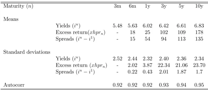
We estimate the model using U.S. macroeconomic as well as term structure data at the quarterly frequency. The sample period is 1962 Q1 -2001 Q2.

The macro data used are per capita real consumption growth, per capita real GDP growth, and Consumer Price Index (CPI) in‡ation rate. Consumption is NIPA measures of personal consumption expenditure on non durable goods and services. Real consumption is obtained by dividing its nominal measure by CPI in‡ation rate. All the macro data are seasonally adjusted and are collected from the Federal Reserve Bank of St. Louis website (www.stls.frb.org).

The term structure of interest rates data are the nominal three-month interest rate and the ten-year nominal interest rate. The three-month rate is daily treasury bill rate whereas the ten-year interest rate is daily constant maturity rate. All interest rates series are from the Federal Reserve Bank of St. Louis website. We obtained quarterly observations by taking the …rst trading day observation of the second month of each quarter6 _{(February, May, August, November). In the estimation, we use the spread}

between the ten-year and the three-month nominal interest rates. Notice that the model counterparts of the three-month and ten-year interest rates are one-period and forty-period interest rates respectively.

1.5.2

Paramaters Estimation : Simulated Method of

Mo-ments (SMM)

We estimate the shocks parameters of the model by the Simulated Method of Moments (SMM). The number of estimated parameters is …ve : the persistence para-meters of technology ( a) and preferences ( u) shocks ; and the standard deviations

of the three shocks u, ", mp. The remaining parameters have been calibrated to

the U.S. economy or set in line with the literature.

SMM consists in minimizing a weighting distance between unconditional moments predicted by the model and the corresponding data moments counterpart. Basically, the predicted moments are based on arti…cial data simulated from the model while data moments are directly computed from actual data. This method is appealing for nonlinear DSGE models estimation because, as shown by Ruge-Murcia (2007), it is robust to misspeci…cations and is computationally e¢ cient. In addition, Lee and Ingram (1991), and Du¢ e and Singleton (1993) show that parameters estimates by SMM are consistent and asymptotically normal. Ruge-Murcia (2012) provides the

properties of SMM estimates for third-order approximation of DSGE models. The Monte - Carlo evidence on small samples shows that SMM based asymptotic standard errors tend to overestimate the actual variances of the parameters. Thus, we use a block bootstrap method to compute a ninety- …ve per cent con…dence intervals for the parameter estimates.

Since SMM analysis requires stationary variables, we simulate the model on the basis of the pruned version of the second-order approximate solution proposed by Kim, Kim, Schaumburg and Sims (2008). The innovations are drawn from the nor-mal distribution for the simulation. The moments used in the estimation are the variances, …rst- and second-order autocovariances of the four data series, in addition to the unconditional mean of the interest rate spreads and the in‡ation rate. Because consumption growth and real GDP growth rates are positive in the U.S. data and there is no growth in the model, we discard the mean of these two variables. Thus, fourteen moments are used in the estimation of the …ve parameters meaning that the number of degrees of freedom is nine. The weighting matrix used is the diagonal of the Newey-West estimator of the long-run variances of the moments with a Bartlett kernel and a bandwidth given by 4(T/100)2=9 _{(as in Ruge-Murcia, 2010). The sample}

size here is T=158 which implied a bandwidth value of 4.427. We simulate …ve times the sample size (T) observations for the arti…cial series.

Before the estimation test whether the series used in the estimation are stationary as the theoretical properties of SMM estimates are valid under this assumption. To this end, we use an Augmented-Dickey Fuller (ADF) and a Phillips-Perron (PP) unit root tests. The null hypothesis of unit root can be rejected at 5% level under both tests for all series except the in‡ation rate. However, for the in‡ation rate, the unit root hypothesis can be rejected at the 5% level under the PP test but cannot be rejected under the ADF test. But the ADF-statistic is -2.38 whereas the critical value is -2.39. So, we suppose that the in‡ation rate is stationary.

1.5.3

Calibration

During the estimation, the remaining model parameters have been calibrated as follow :

The subjective discount factor is parametrized at =0.99 to match the average annual real interest rate of 4%. The consumption curvature coe¢ cient in the utility function is set to a value of = 2:This value is in the range of empirical estimates in the DSGE models literature7_{. The habit strength parameter is set to b = 0:65 as in}

Constantinides (1990), Boldrin, Christiano and Fisher (2001). The labor elasticity is set to ' = 2 and '₀ is calibrated to match 1/3 of steady state hours worked without