Comparative validation of three water cooling coil models

(1)

Comparative and empirical validation of three water cooling coil models

Gendebien Samuel1, Bertagnolio Stephane1 and Lemort Vincent1

1

Thermodynamics Laboratory, University of Liège, Belgium

Corresponding email: sgendebien@ulg.ac.be

SUMMARY

Water cooling coils are widely used in common HVAC systems. Accurate and robust cooling coil simulation models are required to perform reliable calculations of building cooling needs. Many different cooling coil simulation models were developed during the last decades. The most commonly used cooling coil models are presented and compared in terms of implementation in the first part of the paper. A simplified variable boundary model is presented and comparatively and empirically validated to two reference models.

INTRODUCTION

Condensing heat exchangers are widely used in to-air heat exchange applications (e.g. air-to-air heat recovery heat exchangers in air conditioning systems), air-to-water heat exchange applications (e.g. water cooling coils in air conditioning systems) and gas-to-water heat exchange applications (e.g. condensing boilers heat exchangers). Robust, accurate and validated simulation models of condensing heat exchangers are highly needed to perform reliable calculations of building HVAC energy use. The present papers focuses on the application of condensing heat exchanger models to air conditioning water cooling coils. Software developers and researchers developed and validated many water cooling coil models during the last decades. The most commonly used water cooling coil models are:

- Single zone epsilon-NTU models [1,2]. - Variable boundary models [3].

- Finite elements [4] and lumped models.

In the first part of this paper, the most common single zones and variable boundary models will be described and compared in terms of implementation: the “Ashrae Toolkit” model [3], the “Braun-Lebrun” model [1] and the “Morisot” model [2,6]. The second part of the paper presents a simplified variable boundary model adapted from the Ashrae Toolkit [3]. The third part of the paper offers a comparative validation between the later model and two reference single zone models.

COMMON EXISTING MODELS Toolkit model [3]

In the case of a partially wet regime, the Toolkit model divides the heat transfer area of the cooling coil in two parts: a totally dry portion and a totally wet portion. These portions are separated by a mobile boundary, whose position is determined by means of the surface temperature.

(2)

Three operating modes can be identified:

- in totally dry regime, the dry portion covers the whole heat transfer area and the wet portion area is reduced to zero;

- in totally wet conditions, the dry regime portion area is reduced to zero;

- in partially wet conditions, the variable boundary determines the part of the transfer area where condensation occurs.

Under dry conditions, exhaust air and water conditions can be determined using standard heat effectiveness relationships (classical

ε

_{– NTU method) based on the overall heat transfer}

coefficient (AUdry in W/K).

In wet regime, enthalpies are preferred instead of temperatures to determine the cooling capacity of the coil because they are including latent effects. In this model, water enthalpies are replaced by “fictitious fluid” enthalpies, defined as the enthalpy of saturated air at the temperature of the water. Heat transfer in the coil is calculated by the following relationships:

(1)

(2) with

(3)

(4)

where the variable cp;sat is an effective specific heat of saturated air, defined by the following relationship:

(5)

It is important to notice that the rigorous determination of cp;sat requires the knowledge of the surface temperature at the entrance and at the exit of the wet part of the coil. In order to avoid iterations, the dewpoint temperature of the entering air and the supply water temperature are preferred.

The overall enthalpy transfer coefficient can be related to conventional internal and external heat transfer resistances by the following relationship:

(6) Knowing the overall enthalpy transfer coefficient, the air exhaust enthalpy and the water exhaust enthalpy can be determined by the classical

ε

_{– NTU method.}

The leaving air conditions (dry bulb temperature and humidity) are determined by considering a fictitious semi isothermal heat exchanger. One of the two fluids is the air and the other is a fictitious fluid with an infinite capacity rate at the condensate temperature.

The solving procedure determines the cooling capacity by identifying the dry and the wet parts of the coil in the considered operating conditions. Cooling coil is considered as “wet” when the surface temperature is equal to the supply air dewpoint temperature.

The solving procedure is composed of two interlinked iterative loops: Q_coil;wet = C_a;wet · ( h_a;su;coil – h_a;ex;coil) Q_coil;wet = C_w;wet · ( h_{w;sat;su;coil} – h_{w;sat;ex;coil})

Ca;wet = Ma Cw;wet := Mw · cp;w cp;sat cp;sat = h_dp;su;coil – h_{w;sat;su;coil} tdp;su;coil – tw;su;coil AUwet := 1 cp;sat · Rw + cp;a · Ra

(3)

- A first loop iterating on the wet surface area fraction to converge on surface temperature equal to entering air dewpoint at the boundary.

- A second loop iterating on the water temperature at boundary for a given wet surface area fraction.

Braun-Lebrun model [1]

Contrary to the “Toolkit” model, the “Braun-Lebrun” model does not take a variable boundary between the wet and the dry parts of the cooling coil into account. This simpler model considers simultaneously fully dry and fully wet regimes and applies Braun hypothesis by considering that the regime to be considered (totally wet or totally dry) is the one leading to the maximal cooling capacity. Braun [5] showed that this approximation generally leads to an error less than 5% on total energy rate.

(8)

To determine the exhaust air and water conditions under dry regime, the classical

ε

_{– NTU}

method is used once again. In wet regime, in order to take latent effect into account, the air is replaced by a fictitious perfect gas whose enthalpy is fully defined by the actual wet bulb temperature.

The specific heat capacity of the fictitious fluid is given by the following relationship: (9)

The air side thermal resistance is:

(10)

Knowing the wet effectiveness (on the basis of the convective resistance), heat transfer rate is given by:

(11) (12)

with

(13)

As proposed in the “Toolkit” model, a fictitious semi isothermal heat exchanger is once again considered to determine the outlet air conditions. One of the two fluids supplying this heat exchanger is the air; the other one is a fictitious fluid of infinite capacity flow rate, whose uniform temperature is supposed to correspond to the average temperature of the external surface of the coil, also called “contact” temperature.

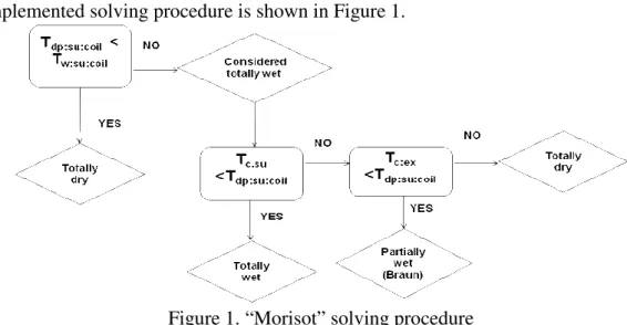
Morisot model [2, 6]

Morisot proposed a combination of the “Toolkit” model and the “Braun-Lebrun” model. The characteristics of this third model are:

- The wet regime is described in the same way than the “Toolkit” model.

Qcoil = Max ( Qcoil;dry ; Qcoil;wet )

c_{p;a;f ;coil} = ha;su;coil – ha;ex;coil;wet twb;su;coil;coil – twb;ex;coil;wet

R_{af ;coil} = R_a;coil · cp;a;coil c_{p;af ;coil}

Q_coil;wet = ε_coil;wet · C_min;coil;wet · ( t_wb;su;coil – t_r;su;coil) Q_coil;wet = C_{af ;coil} · ( t_wb;su;coil – t_{wb;ex;coil;wet} )

(4)

- The model is based on the Braun-Lebrun method which consists in determining simultaneously the cooling capacity by assuming the coil completely dry or completely wet and to choose the regime leading to maximal heat transfer rate.

The implemented solving procedure is shown in Figure 1.

Figure 1. “Morisot” solving procedure SIMPLIFIED VARIABLE BOUNDARY MODELS

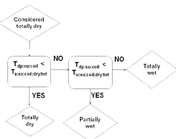
The philosophy of this model is based on the Toolkit one. As proposed in the Toolkit model, it divides the heat transfer area of the cooling coil in two parts: a totally dry portion and a totally wet portion. But contrary to the toolkit one, the surface temperature doesn’t take part in the determination of the dry part of the exchanger: it is assumed that the temperature of the air at the boundary is equal to the dew point temperature at the heat exchanger inlet, as illustrated in figure 2.

Figure 2. Representation of the dry and wet parts of the cooling (for the simplified variable boundary model)

Another difference between this model and the Toolkit one is also the way to describe the wet regime. Like in Braun-Lebrun method, the air is replaced by a fictitious perfect gas whose enthalpy is fully defined by the actual wet bulb temperature. The solving procedure of this model is given in Figure 3.

(5)

Figure 3. Solving algorithm of the simplified variable boundary model IDENTIFICATION OF MODELS PARAMETERS

The parameters of the models mentioned above are:

- The air-side heat transfer coefficient in rating conditions - The water-side heat transfer coefficient in rating conditions - The metal thermal resistance (supposed constant)

Two methods are commonly used to identify the values of these parameters:

- Semi-empirical parameter identification using one or several operating points to calibrate the parameters of the simulation model. The use of the operating points is often combined to practical assumptions (e.g. ratio between water-side and metal thermal resistances).

- Deterministic parameter identification relying on empirical correlations based on the geometrical characteristics of the considered coil.

Only the semi-empirical parameter identification method is considered in this paper. This method has been well described in the case of the Braun-Lebrun model in the IEA-ECBCS Annex 43 project [7]. Among others, it was shown that one only single point (such as the nominal manufacturer performance point) does generally not constitute enough information to accurately identify the 3 heat transfer coefficients. Actual performance may also differ from those stated in the manufacturer submittal due to fouling of the cooling coil (that increases the metal resistance).

VALIDATION OF THREE COOLING COIL MODELS

Three models are investigated during the validation: the Braun-Lebrun one, the Morisot one and the simplified model boundary one. The implementation and the validation of the three models have been realized by means of EES [8]. Performance points considered for validating the models come from experimental data collected by Morisot [2]. Except the water flow rate which is almost constant (0.639 kg/s), all the physical quantities are variable. The inlet air temperature is comprised between 17.2 °C and 23.6 °C and the inlet water temperature is comprised between 7.6 °C and 11.3 °C.

The metal thermal resistance was neglected for the three validations. The identified parameters of the three models are:

(6)

- the air-side heat transfer coefficient in rating conditions - the water-side heat transfer coefficient in rating conditions The validation is based on four parameters:

- the total energy exchanged by the water flow and the air stream: - the sensible heat ratio: SHR

- the exhaust water temperature: Tex;w;coil

- the exhaust air temperature: Tex;a;coil

“Braun-Lebrun” model 0 1000 2000 3000 4000 5000 6000 7000 8000 9000 10000 0 1000 2000 3000 4000 5000 6000 7000 8000 9000 10000 Q_meas Q Q Q a) 0 0,1 0,2 0,3 0,4 0,5 0,6 0,7 0,8 0,9 1 1,1 0 0,1 0,2 0,3 0,4 0,5 0,6 0,7 0,8 0,9 1 1,1 SHR_meas S H R SHR SHR b)

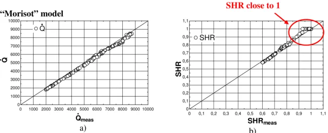
Figure 4. Experimental validation of the “Braun-Lebrun” model. a) cooling capacity and b) SHR “Morisot” model 0 1000 2000 3000 4000 5000 6000 7000 8000 9000 10000 0 1000 2000 3000 4000 5000 6000 7000 8000 9000 10000 Q_meas Q Q Q a) 0 0,1 0,2 0,3 0,4 0,5 0,6 0,7 0,8 0,9 1 1,1 0 0,1 0,2 0,3 0,4 0,5 0,6 0,7 0,8 0,9 1 1,1 SHR_meas S H R SHR SHR b)

Figure 5. Experimental validation of the “Morisot” model. a) cooling capacity and b) SHR

SHR close to 1

(7)

Simplified variable boundary model 0 1000 2000 3000 4000 5000 6000 7000 8000 9000 10000 0 1000 2000 3000 4000 5000 6000 7000 8000 9000 10000 Qmeas Q Q Q a) 0 0,1 0,2 0,3 0,4 0,5 0,6 0,7 0,8 0,9 1 1,1 0 0,1 0,2 0,3 0,4 0,5 0,6 0,7 0,8 0,9 1 1,1 SHRmeas S H R SHR SHR b)

Figure 6. Experimental validation of the variable boundary model. a) cooling capacity and b) SHR

DISCUSSION Parameters

If metal resistance is neglected, all the validated models only necessitate two parameters (the airside and the waterside heat transfer coefficients. The values of the identified model parameters are given in table 1:

Table 1: Heat transfer coefficients

Air heat transfer coefficient Water heat transfer coefficient “Braun-Lebrun” model AUa;n = 2000[W/K] AUw;n = 1850[W/K]

“Morisot” model AUa;n = 2415 [W/K] AUw;n = 1768 [W/K]

SVB model AUa;n = 6000 [W/K] AUw;n = 1387 [W/K]

Accuracy

Root mean squared of the errors on the temperatures (RMSE) and coefficient of variation of the root mean squared of the errors on heat transfer rates (CV(RMSE)) are given in Table 2. It appears that the three models provide satisfying results, in the range of values of the uncertainties on measured energy rate (+/- 200W) and temperatures (+/- 0.3 K) [2].

Table 2: RMSE and CV(RMSE)

Braun-Lebrun Morisot Variable boundary Cooling capacity [W] CV(RMSE): 3.5 % CV(RMSE): 4.9% CV(RMSE): 3.0 % SHR [%] CV(RMSE): 1.9 % CV(RMSE): 2.0 % CV(RMSE): 1.6 % Leaving Air Temp. [C] RMSE: 0.22 K RMSE: 0.28 K RMSE: 0.28 K Leaving Water Temp. [C] RMSE: 0.13 K RMSE: 0.17 K RMSE: 0.07 K As shown in Figures 4 and 5, the “Braun-Lebrun” and the “Morisot” models have good behavior and performance predictions. The main problem of these two models is that they are not able to represent cooling coil operation for a sensible heat ratio (SHR) around 1. In fact, this problem comes from the Braun’s hypothesis: for SHR closed to one, Braun method assumes the coil completely dry. This approximation does not affect global simulation results. On the contrary, the simplified variable boundary model produces good results even for SHR closed to one (Figure 6). This could be very interesting for simulating devices such as

(8)

air recuperative heat exchanger where the knowledge of the condensing water flow rate is very important even for SHR closed to one. The condensing water could obstruct the air passage and create a pressure drop that could decrease the ventilation rate.

CONCLUSION

The three studied and validated models produce good performances prediction. In general, use of Morisot and Braun-Lebrun models will be preferred because of their easier implementation. But use of the simplified variable boundary model is also interesting, especially if the SHR is closed to one. For example, this model could be applied to calculate the performance of an air-to-air recuperative heat exchanger. Simulation of condensing boilers heat exchangers could also be an application of this simplified variable boundary model if coupled to a combustion chamber model.

NOMENCLATURE

Variables

AU: heat transfer coefficient, W/K

c: specific heat, J/(kgK) : capacity flow, W/K ε_{: effectiveness, -}

h: specific enthalpy, J/kg : mass flow rate, kg/s

NTU: number of transfer unit, - : heat transfer, W

R: thermal resistance, K/W

SHR: sensible heat ratio, -

T: temperature, °C w: humidity ratio, kg/kg Subscripts a: air c: contact coil: coil dp: dewpoint

dry: dry portion, dry regime

ex: exiting, leaving, outlet

f: fictitious meas: measured min: min sat: saturated w: water wb: wetbulb

wet: wet portion, wet regime

REFERENCES

1. Lebrun, J., X. Ding, J.-P. Eppe, and M.Wasac. 1990. Cooling Coil Models to be used in Transient and/or Wet Regimes. Theoritical Analysis and Experimental Validation. Proceedings of SSB 1990. Liège:405-411

2. Morisot, O., Marchio, D. (2002). Simplified Model for the Operation of Chilled Water Cooling Coils Under Nonnominal Conditions. HVAC&R Research 8(2): 135-158.

3. Brandemuehl, M.J., S. Gabel, and I. Andersen. 1993. A toolkit for secondary HVAC System Energy Calculations. Published for ASHRAE by Joint Center for Energy Management, University of Colorado at Boulder.

4. Wang, G., M. Liu, and D. Claridge. 2007. Decoupled modeling of Chilled-Water cooling coils, ASHRAE transaction 113(1).

5. Braun, J.E. 1988. Methodologies for the design and control of central cooling plants. Ph.D. dissertation. University of Wisconsin, Madison.

6. Morisot, O. 2000. Modèle de batterie froide à eau glacée adapté à la maîtrise des consommations d’énergie en conception de bâtiments climatisés et en conduite d’installation. Ph D. Thesis. 7. Lemort, V., Rodríguez, A. and Lebrun, J. 2008. Simulationcof HVAC Components with the

Help of an Equation Solver, Final Report of the IEA Task34/Annex43 Subtask D, University of Liège, Belgium.