Logic and Linear programs to understand cancer response

HAL Id: hal-01897036

https://hal.archives-ouvertes.fr/hal-01897036

Preprint submitted on 16 Oct 2018

HAL is a multi-disciplinary open access

archive for the deposit and dissemination of

sci-entific research documents, whether they are

pub-lished or not. The documents may come from

teaching and research institutions in France or

abroad, or from public or private research centers.

L’archive ouverte pluridisciplinaire HAL, est

destinée au dépôt et à la diffusion de documents

scientifiques de niveau recherche, publiés ou non,

émanant des établissements d’enseignement et de

recherche français ou étrangers, des laboratoires

publics ou privés.

Logic and Linear programs to understand cancer

response

Misbah Razzaq, Lokmane Chebouba, Pierre Le Jeune, Hanen Mhamdi, Carito

Guziolowski, Jérémie Bourdon

To cite this version:

Misbah Razzaq, Lokmane Chebouba, Pierre Le Jeune, Hanen Mhamdi, Carito Guziolowski, et al..

Logic and Linear programs to understand cancer response. 2018. �hal-01897036�

cancer response

Misbah Razzaq, Lokmane Chebouba, Pierre Le Jeune, Hanen Mhamdi, Carito Guziolowski, and J´er´emie Bourdon

Abstract Understanding which are the key components of a system that distinguish a normal from a cancerous cell has been approached widely in the recent years us-ing machine learnus-ing and statistical approaches to detect gene signatures and predict cell growth. Recently, the idea of using gene regulatory and signaling networks, in the form of logic programs, has been introduced in order to detect the mechanisms that control cells state change. Complementary to this, a large literature deals with constraint based methods for analyzing genome-scale metabolic networks. One of the major outcome of these methods concerns the quantitative prediction of growth rates under both given environmental conditions and the presence or absence of a given set of enzymes which catalyze biochemical reactions. It is of high importance to plug logic regulatory models into metabolic networks by using a gene-enzyme logical interaction rule. In this work, our aim is first to review previously proposed logic programs to discover key components in the graph based causal models that distinguish different variants of cell types. These variants represent either cancerous vs. healthy cell types, multiple cancer cell lines, or patients with different treatment response. With these approaches, we can handle experimental data coming from transcriptomic profiles, gene expression micro-arrays or RNAseq, as well as (multi-perturbation) phosphoproteomics measurements. In a second part, we deal with the problem of combining both, regulatory and signaling, logic models within metabolic networks. Such a combination allows us to obtain quantitative prediction of tumor cell growth. Our results point to logic program models built for 3 cancer types: Mul-tiple Myeloma, Acute Myeloid Leukemia, and Breast Cancer. Experimental data for

Misbah Razzaq · Pierre Le Jeune · Carito Guziolowski ( )

LS2N, UMR 6004, ´Ecole Centrale de Nantes, Nantes, France., e-mail: Carito.Guziolowski@ls2n.fr Lokmane Chebouba

Department of Computer Science, LRIA Laboratory, Electrical Engineering and Computer Science Faculty, University of Science and Technology Houari Boumediene (USTHB) El-Alia BP 32 Bab-Ezzouar, Algiers, Algeria

Hanen Mhamdi · J´er´emie Bourdon ( )

LS2N, UMR 6004, Universit de Nantes, France. e-mail: Jeremie.Bourdon@univ-nantes.fr

these studies was collected through DREAM challenges and in collaboration with biologists that produced them. The networks were built using several publicly avail-able pathway databases, such as Pathways Interaction Database [37], KEGG [17], Reactome [10], and Trrust [13]. We show how these models allow us to identify the key mechanisms distinguishing a cancerous cell. In complement to this, we sketch a methodology, based on currently available frameworks and datasets, that relates both the linear component of the metabolic networks and the logical part of logic programing based methods.

1 Introduction

Patients suffering from cardiovascular, inflammatory, oncology, infectious, and neu-ropsychiatric human diseases present a vast heterogeneity in their genome and gene or protein expression profiles. Regulatory networks (describing protein, gene, and metabolic regulations) may not necessarily be wired in the same way for two dif-ferent individuals. Therefore, a concrete treatment may not show the same effect in all patients and in some cases, such as cancer for example, it can encourage disease progress. Classical medical approaches to treat disease provide fixed protocols of treatment independent of the patients heterogeneity. Systems Medicine is a recent field of research that proposes disease regulatory networks as explanations on how the genes or protein express in an individual. On this way, network analyses shall provide a disease molecular signature that can be connected to clinical observa-tions. While past diagnosis methods focused only on measuring single parameters, the premise of Systems Medicine is to perform multi-parameter analyses that may result on a more plausible explanation of disease. This novel research field is rein-forced by the fact that current technology allows us to measure the state of several species in these regulatory networks in a high-throughput fashion. In this context we review and discuss here recently published methods to compute disease signa-tures in computational models, built from patients and cell lines gene or protein expression profiles. The models we propose combine logic and linear programming techniques.

The exponential increase of biological data (genomic, transcriptomic, proteomic) [27] and of biological interaction knowledge in Pathway Databases allows model-ing cellular regulatory mechanisms. Modelmodel-ing biological mechanisms is done, most of the time, using boolean or ordinary differential equation representations. Those approaches have shown their efficiency in cellular phenomena study [6], disease research [24, 33], and bio-production optimization [4]. However, those modeling approaches cannot take into account the large amount of OMIC data. This limita-tion requires that the researcher preselects the OMIC data and network, adding bias to the analysis [31]. In this study we review a modeling approach named perfect coloring, which is based on exhaustive and global graph coloring approaches [41]. These approaches are able to predict the graph coloring configurations, in terms of discrete states (e.g. active or inactive) of the molecular species of a biological

network with respect to a set of experimental observations. The perfect coloring modeling approach extends those approaches by looking for harmonious or perfect coloring models. We illustrate how this method can be used for Multiple Myeloma understanding and patients prognosis classification.

Patients’ response classification is usually approached by methods that find sta-tistically significant markers from the transcriptomic or proteomic data at hand. A classical method used for this is univariate and multivariate Cox proportional haz-ards analyses. Following such approach, several statistic [20, 46] and machine learn-ing [23, 12, 32] methods conceived for significant features extraction have been ap-plied to this problem. More recent approaches include the notion of pathways in this drug detection problem [3]. Such methods allow identifying the regulatory mecha-nisms related to the best drug targets [19] and this mechanistic information is valu-able to understand the disease and the complexity of drug targeting. We have intro-duced in [44] the caspo method, which learns Boolean networks (BNs) from phos-phoproteomic multiple perturbation data by using logic programming. This frame-work allows us to retrieve families of BNs having the best fit to the experimental data from exhaustive searches over a large-scale Prior Signaling Network. In this work we review a method that allows caspo to handle patients data. In fact, caspo needs as input data proteins measurements across multiple perturbations. While such datasets are possible to obtain for cell lines, they are impossible to obtain for patients. How-ever, by preselecting partial measurements of the complete patients dataset, we may retrieve cases where the protein observations behave as if they were perturbed in a same way for different treatment response classes of patients. We discuss here how this approach is suitable to find the mechanisms differentiating the complete remission and primary resistant responses of Acute Myeloid Leukemia patients.

Traditional canonical signaling pathways help to understand overall signaling processes inside the cell. Large scale phosphoproteomic data provide insight into al-terations among different proteins under different experimental settings. The caspo time series (caspo-ts) method, provides a framework to combine the traditional sig-naling networks with complex phosphoproteomic time-series data in order to un-ravel cell specific signaling networks. We have applied the caspo-ts approach, which is a combination of logic programming and model checking, over the time series phosphoproteomic dataset of the HPN-DREAM challenge to learn cell specific BNs. In this work we give an overview of this framework and show the Boolean networks (BNs) learned from the BT549 breast cancer cell line. The learned BNs can be used to identify the cell specific topology. caspo-ts scales to real datasets, usually with in-herent noise, outputting networks that are cell specific. It can be thus used to identify the cell specific and common mechanisms (logical gates) when comparing multiple cell lines.

Finally, after presenting and discussing linear programmling approaches in the context of metabolic network analyses, we provide a sketch of a hybrid method-ology, based entirely on published results. This hybrid model combines linear and logic programming to model drug effects in a multi-layer network including regula-tory, signaling and metabolic events.

2 Regulatory and Signaling networks as Logical programs

In the following we review and discuss three recently proposed methodologies to understand medical data using models. The models presented here are of discrete nature, implemented as logic programs in Answer Set Programming (ASP) [5]. In the first approach we built a model integrating gene regulatory networks and ex-perimental observations as facts in a logic program interpreted by checking the sat-isfiability of a constraint named perfect coloring. In the second, we used Boolean networks to model the fact of reproducing the experimental observations with min-imal error. While the perfect coloring model is applied for large-scale (thousands of components) networks and gene expression observations, the Boolean models are applied on middle-scale case studies (hundreds of components) using either pro-teomics data measured across several patients or multiple perturbation time-series phosphoproteomics datasets measured across cell lines.

2.1 Perfect coloring model

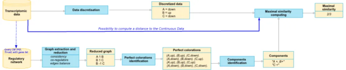
This methodology was introduced in [30]. The main steps of this method are pre-sented in Fig. 1.

Fig. 1 Overview of the perfect coloring modeling framework. Blue boxes refer to processing steps and yellow boxes refer to input/output data.

This method works exclusively on the discrete model underlying a regulatory network, and avoids preprocessing the experimental data. The analysis of such a model will predict subgraphs or graph components that are independent according to the up- or down-regulated coloring of their nodes. The input of this method is a graph G(V, E) composed of a set of nodes V and edges E; where an edge is a tuple with 2 nodes (source and target), a sign (1 for activation, -1 for inhibition) and a weight. Such graphs can be obtained from publicly available databases, such as the Pathway Interaction Database [40] and Trrust [14] by querying a predefined list of genes. The perfect coloring approach can be summarized in 4 steps:

1. Reduce a large-scale graph by restricting the search space associated to this graph. For this, several graph operations are applied that remove redundant nodes

or paths. Such graph nodes or edges will be redundant with respect to the perfect

coloringconstraint.

2. Once the size of the graph was reduced, the next step is to enumerate all the possible ways to color the graph in a perfect (or harmonious) way. In a colored graph all nodes will be associated to a sign: up standing for ”+” and down for ”-”. These signs refer to the qualitative variation that can be experimentally mea-sured in a molecular species of the graph when comparing 2 cellular states, for example after and before a stress condition. In this work we were interested on modeling sets of possible state variations of the graph nodes that satisfy a perfect

coloringconstraint. The intuition behind this constraint is to point to network

discrete variation states that maximize the agreement between a target molecular species up or down variation and the positive or negative influence from its reg-ulators in the graph. The perfect coloring constraint can be expressed in natural language as follows: ”for a given node in the graph we impose that its discrete up or down-regulation is explained by a similar (positive or negative) influence from a maximal number of direct predecessors”. This statement is inspired from a hypothesis of redundancy in biological networks control, and we use ASP to express this statement and search for coloring models where this property holds for every node in the graph.

3. Among the possible coloring models that satisfy the perfect coloring constraint, many of them can be clustered together on account of the symmetry of our ap-proach created by the duality of our knowledge representation: positive-negative influence (edges), up- or down-regulation of molecular species states (nodes). Clustering the perfect coloring configurations allows us to build subgraphs or graph components that drastically reduce the dimensionality of our data; and consequently to focus on a very reduced set of comparisons with respect to ex-perimental data.

4. The last step consists on measuring how the up or down-regulation coloring of the nodes in the subgraphs compare to the experimental data. As shown in Fig. 1, this comparison can be done without discretization of the experimental data, by measuring a distance between the discrete coloring and the continuous data. Step 1 is implemented on Python 2.7, step 2 on ASP (clingo 4.5.4), and steps 3-4 on R and Python 2.7. A usage example and the sources of this method are publicly available at [28].

2.1.1 Patient classification

Given a patient gene expression profile (GEP) and given a regulatory network G, the perfect coloring approach described above, can propose a similarity vector of size k, where k is the number of components identified for G. This similarity vector is specific to the patient expression profile, and could be understood as a vector of features. Given a cohort of patients, in which each patient is assigned a good or bad prognostic label, we can use machine learning techniques to learn a classifier from the similarity feature vectors of all patients in a training database. This classifier can

predict when a new patient arrives, the patient’s good or bad prognostic according to the training patient set. We have implemented a software named IGUANA publicly available for Windows and Mac OS in which such classifier is built using XGBoost (Extreme Gradient Boosting). A complete user guide and use case examples are provided online at [21]. Our objective here was to provide the complete framework via a user-friendly human interface.

2.1.2 Case study - Multiple Myeloma

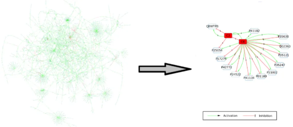
Multiple myeloma (MM) is a hematologic malignancy representing 1% of all can-cer [38] with a survival rate of 49.6% after 5 years. The perfect coloring method was applied to transcriptomic data from myeloma cells (MC) of 602 MM patients and from normal plasma cells (NPC) of 9 healthy donors [29]. We used the PID-NCI database to generate a graph by extracting the downstream events from three signaling pathways (IL6/IL6-R, IGF1/IGF1-R and CD40) to significantly differen-tially expressed genes of the patients profiles. The obtained subgraph from NCI-PID 2012, contained 2269 nodes, 2683 edges and connected 529 differentially expressed genes. The perfect coloring method identified 16384 coloring models, grouped in 15 components or subgraphs (see Fig 2). One of these components (422 nodes and 167 genes) was found statistically specific to MC in comparison to NPC. Using gene ontology enrichment analysis with PANTHER [43] we were able to associate this component to oncogenic phenomena.

Fig. 2 Components identification by perfect coloring approach. Left: subgraph obtained from the PID-NCI database (2269 nodes, 2683 edges). Right: 15 components identified from all the per-fect coloring models. The components composed only with one gene are labeled with the Uniprot identifier.

The perfect coloring approach and the classifier was applied to the data of the

Multiple Myeloma DREAM challenge1. The objective of this challenge was to

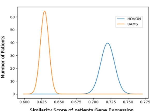
clas-sify the MM patients labeled as high risk. They provided to the methodological community large MM patient cohorts (25000 patients) where patient gene expres-sion profiles and risk information were measured by different US laboratories. We tested our method with 2 sets of gene expression profiles: HOVON (GSE19784, 274 GEPs) and UAMS (GSE24080, 558 GEPs). The graph was a gene regulatory network generated with the Trrust database by querying the significantly expressed genes in the intersection of both datasets. The graph of 447 nodes and 600 edges, was reduced to 30 components with the perfect coloring approach. After this, we ap-plied XGBoost to learn a classifier from the HOVON dataset to predict the UAMS dataset and vice versa, and obtained precision rates of 0.75 and 0.71 respectively. Our precision rate was not satisfactory when comparing it to the one obtained by the other teams participating in the DREAM challenge using gene expression profiles provided by different research institutes, other than HOVON and UAMS. We be-lieve our method is very sensitive to the initial graph; it is important that this graph contains all the significantly expressed genes across all GEPs provided by all the research centers. We were unable to verify this since for this DREAM challenge in particular the testing data is not made available to the community. Finally, this approach can be used to study divergences among the datasets provided by different experimental platforms or in this case by different research laboratories. Such study is crucial to check if multiple datasets can be merged in order to create a larger one. A large set would provide more training examples for the perfect coloring model, and this would certainly improve its accuracy. For this, we calculated the expected value as well as the standard deviation for the distributions of similarity scores for each of the 30 components across both sets of profiles (HOVON vs. UAMS). We ob-serve that 7 out of 30 distributions have an expected value of the similarity score at a distance equal or greater than 0.07, such as component 7 for example (see Fig. 3). This means that we can identify regulatory mechanisms within the network pointing to regions where the experimental data provided diverges. Note that in this analysis, we supposed that the similarity scores of each component are normally distributed, so that we are able to plot their distributions and compare them. Similarity scores are linear combinations of gene expression levels and they will be normally distributed if and only if all gene expression levels can be modeled as independent random variables normally distributed.

2.2 Caspo for discovering Boolean networks distinguishing

different classes of patients data

In this section we review a method [9] based on ASP and caspo to predict the Boolean models associated to patients holding separate diagnostics: complete

Fig. 3 Distribution of similarity score from the perfect coloring approach across two ex-pression profiles of two different patient cohorts (UAMS and HOVON) for the same graph component. The perfect coloring method detected 30 components in the graph obtained from the Trrust database using the differentially expressed genes of the gene expression profiles (GEP) of 2 research centers (UAMS, HOVON). These GEPs were provided by the Multiple Myeloma DREAM challenge. The similarity scores of each patient with respect to the genes of the compo-nent are shown in the x-axis and represent how the perfect coloring values from the compocompo-nent match the continuous data of the GEPs provided by both independent platforms.

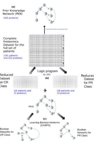
mission (CR) and primary resistant (PR). This method receives as input information a Prior Knowledge Network (PKN) and a experimental dataset consisting of protein measurements associated to several patients. It consists of four steps (see Fig. 4). 1. Creation of a PKN. We used public databases to connect the measured proteins.

The PKN is composed of 3 types of nodes: stimuli are the entry of the network (nodes without predecessors), readouts are the output of the network (nodes with-out successors) and inhibitors are proteins in between the entry and with-output net-work layers.

2. Protein and patient selection. This step executes a logic program implemented in ASP that selects a group of k stimuli and inhibitor proteins that maximize the number of pairs of patients for which the binarized values of their experimental measures matched in both classes (CR, PR) and where the difference of readouts measures for each class is maximal.

3. BNs learning. We used the dataset issued from step 2 to learn BNs with caspo [45]. This step produces two families of BNs, one for the CR class and the other for the PR class. Our objective here was to learn different families of BNs by using the identical stimuli-inhibitor cases and the maximal difference of read-outs measures for each class and finally compare the structure and mechanisms between these BNs families.

4. Classification. The set of unseen patients was classified by using our learned logic models. For this we computed the Mean Square Error (MSE) between mea-sured readouts and predicted readouts for each patient in the testing data based

Fig. 4 Workflow of our method. (a) PKN construction. In this step we pass the proteins present in our DREAM 9 dataset as input to the Cytoscape plug-in Reactome FI to construct the PKN. This plug-in finds all the paths between the input proteins across several databases, after that we select only relations coming from KEGG. (b) Protein and patient selection. This step consists on selecting k proteins from the dataset for which there is a maximum number of pairs of patients that have identical values in the k proteins but that belong to different response classes. (c) Learning. This step consists on finding the BNs for the two classes CR-PR corresponding to the two datasets obtained in step (b).

on the two families of the previously learned BNs. The given patient will be classified in the class with the lower MSE.

2.2.1 Case study - Acute Myeloid Leukemia

In 2014 the DREAM 9 challenge was launched in order to predict the complete re-mission (CR) and primary resistant (PR) response to chemotherapy of 191 Acute Myeloide Leukemia (AML) patients from their proteomics data (231 measured

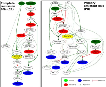
pro-teins) and from 40 clinical data [34]. We describe here how we applied the method sketched in Fig. 4 to the DREAM 9 challenge dataset. First we create a PKN com-posed of 102 nodes (17 stimuli, 62 inhibitors and 23 readouts) connected by 294 edges. The second step of our method, allowed us to select a subset of k = 10 pro-teins extracted from the union of the stimuli and inhibitors present in the PKN (79 proteins), the chosen k maximized the number of pairs of patients belonging to the CR and PR classes. Then we learned the 2 families of BNs using the reduced dataset from the previous step. The CR family had 10 BNs, while the PR one had 9. The size (number of logic clauses) of the optimal BNs for the CR case was of 24, while it was of 29 in the PR BNs (see Fig. 5). When comparing both networks, we can see that the normal growth factor - fibronectin - PI3K pathway in primary resistant pa-tients is better connected to other network components (see yellow node in Fig.. 5). This finding suggests an important rewiring of the PI3K pathway in primary resis-tant patients compared to complete remission ones. This goes in agreement with previously published literature on AML treatment by targeting the PI3K pathway [42].

Fig. 5 Union of optimal BNs learned from the initial PKN and the reduced patients dataset from the complete remission (CR) and the primary resistant (PR) classes. The thicker edges represent those that are the most frequent paths in the BN family. The association between a node and its predecessors is an AND gate if it is preceded by a filled black circle and an OR gate other-wise. Left: Boolean networks for CR patients. This BN can explain and predict the measurements of readouts STMN1 and GAPDH starting from the stimuli FN1 and SMAD6, passing by the in-hibitors LEF1, ERBB3, IGF1R and MAPK9, and other intermediate proteins. Right: Boolean net-works for PR patients. This BN explains and predicts the measurement of readouts PTGS2, TSC2, BAK1 and CASP3 starting from the stimuli FN1, YAP1 and STK11, passing by the inhibitors ERBB3, IGF1R and CASP9, and other intermediate proteins.

2.3 Caspo-ts for discovering Boolean networks distinguishing

time-series data of cell lines

The caspo time series (caspo-ts) method uses Answer Set Programming and Model Checking techniques to solve combinatorial optimization problems of enumerat-ing a family of Boolean networks (BNs) optimally explainenumerat-ing time-series data [35]. Fig. 6 shows the overall process of caspo-ts, a publicly available software at [39]. In the following, we describe briefly the implementation of the main components of

caspo-tsas well as of a recently implemented version of caspo-ts allowing

diversi-fication in the exploration of the solution space of candidate BNs.

Fig. 6 Caspo-ts workflow. Prior Knowledge Networks (PKNs) are extracted from literature cu-rated databases containing information about interactions between different proteins or genes. PKNs are available in different databases such as Reactome, PID, etc. Phosphoproteomic time-series data show the measurement of different proteins at different time points under multiple perturbations. A BN consists of a set of nodes where a Boolean function is assigned to each node. The state of each node is updated by evaluating the Boolean function. Given phosphoproteomic time series data we construct a PKN by querying pathway databases. After normalizing the time series data, we use it together with the PKN as input of caspo-ts (ASP component) for learning BNs. Finally, caspo-ts, uses a model checking step to filter false positive BNs. In this figure the 2 main components of caspo-ts are shown in orange.

1. caspo-ts: ASP component. Given a PKN and a phosphoproteomic dataset, a fam-ily of candidate BNs, compatible with this PKN, is exhaustively enumerated. Af-terwards an over-approximation constraint is imposed upon each candidate BN to filter out invalid BNs [35], that do not result in an over-approximation of the reachability between the Boolean states given by the phosphoproteomic dataset. Finally, an optimization step is performed to select those BNs having a minimal distance between the actual time series and the over-approximated time series. 2. caspo-ts: Model checking component. Because of the over-approximation of

reachability, some of the returned BNs may not reproduce the time-series traces. Such false positives can be ruled out using a model-checking part of the method, leaving us with true positive BNs. True positive BNs are guaranteed to reproduce all traces of the phosphoproteomic time-series data. Model checking was imple-mented through computational tree logic. Existential and future logic operators

were nested in a logic formula to check reachability of traces within BNs. Se-quential reachability is always slow to verify, especially in the case of large scale networks. We have improved this step to reduce the computational time of true positive BNs detection by parallelizing the reachability conditions.

3. caspo-ts with diversification. Since the ASP solver uses a backtracking algorithm to exhaustively generate solutions, it can lead to a situation where successive so-lutions share very similar properties. This can be problematic specially in the case of a large solution space where discovering or analyzing all solutions becomes computationally hard. To resolve this issue, a diverse enumeration scheme has been introduced. This feature has been implemented in caspo-ts and allows to break up the cluster of similar solutions, hence generating diverse solutions.

2.3.1 Case-Study - Breast Cancer

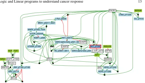
We show an application of caspo-ts with diversification on the BT549 breast cancer cell line. The phosphoproteomic data for this cell line was downloaded from the

DREAM 8 challenge [15, 16]2. In Fig. 7, we show a family of 14 BNs merged

together to represent the signaling behavior of this cell line. For this cell line, we discovered 30 boolean functions. This BN can be executed to understand existing behavior and to predict new behaviors as well.

3 Linear programming approaches in the context of Metabolic

Network Analysis

Nowadays, there has been a huge effort from the community to produce high quality metabolic networks for a wide variety of organisms, tissues or cells. Applications include in-silico metabolic engineering on bacteria, therapeutic target predictions in cell specific metabolic models or gut micro-environment analysis [1, 26] for in-stance. The common feature of all these methods concerns a description of the prob-lem to be studied by using tools from the linear programming theory.

3.1 Metabolic networks as linear systems

Many references already described the linear component of metabolic networks, see [7] for a review. Here, we aim at providing the essentials of such a description.

2 http://dreamchallenges.org/project/dream-8-hpn-dream-breast-cancer-network-inference-challenge/

BCL2L1 . BAD_pS112 EGFR_pY992 MAPK3 . . . c-Raf_pS338 MEK1_pS217_S221 . mTOR_pS2448 AKT_pS473 . p70S6K_pT389 4EBP1_pS65 . . MAPK_pT202_Y204 . GSK3-alpha-beta_pS21_S9 . AKT_pT308 . . GSK3-alpha-beta_pS9 CASP9 . . c-JUN_pS73 . CASP3 SMAD3 AR HER3_pY1298 Rb_pS807_S811 HGF . . BCL2 . c-Met_pY1235 IGF1 . . IRS1 PIK3R1 . Src_pY416 . . HER2_pY1248 JNK_pT183_pT185 NRG1 INSULIN EIF4E FGF1 SERUM

Fig. 7 Union of 14 true positive BNs obtained using caspo-ts on the BT549 breast cancer cell line data. The aggregated BN consists of four different types of nodes: stimuli (green), in-hibitors (red), readouts (blue) and unobserved nodes (white). Stimuli serve as an interaction point for the experimentalists. Inhibitors are blocked through out the experiment. Readouts are measured against a combination of stimuli and inhibitors. Edges are used to represent the type of interaction: positive (green) or negative (red). AND gates are represented by black rectangles where the nodes of incoming edges are their elements.

3.1.1 Metabolic reactions and stoichiometric matrix

In this section, one deals with metabolic networks that are defined by the set of biochemical reactions (consumptions and productions of diverse metabolites) that are to be produced in the cell. Typically, a biochemical reaction has the form

2A + 3B −→ 5C + D,

where A, B,C and D are metabolites and -2, -3 are the stoichiometric coefficients of the substrate of the reaction and 5 and 1 are the respective stoichiometric co-efficients of the product of the reactions. More formally, a metabolic network is

defined by a set of metabolitesM , a set of reactions R and a stoichiometric matrix

S= (sm,r)m∈M ,r∈R, where sr,m is the stoichiometric coefficient of metabolite m in

reaction r if m is a substrate or a product of r and 0 otherwise. The stoichiometric matrix plays a major role in the study of metabolic networks. Indeed, the metabolite

concentrations evolutions over time, denoted here as C(t) = (cm(t))m∈M, expresses

as

dC(t)

dt = SV (t), (1)

where V (t) = (vr(t))r∈R is the vector of reaction flux rates.

Notice that the reactions flux rates can be under the influence of catalyzers, which

the set of all proteins having an influence on a reaction of the metabolic network C ⊂ I × R is the set of pairs describing the influences on the metabolic reactions.

Intuitively, if (i, r) ∈C , then presence of protein i has an effect on the rate of reaction

r. Notice that a reaction can be influenced by several proteins and the same protein can have effect on several reactions.

3.1.2 Steady-state hypothesis and Flux cone

At this point, it is important to distinguish between two types of metabolites: inter-nal and exterinter-nal. Exterinter-nal metabolites are all the metabolites allowing an exchange between the cell and its environment. Internal metabolites are the others. For the external metabolites, it is relevant to add exchange reactions of the form ”−→ m”.

Even if the set R and thus the stoichiometric matrix S differs when adding such

reaction, we will still keep the same notations in the sequel when no confusions are possible. The steady-state approximation states that there is no accumulation of metabolites in the system over time. Imposing a constant metabolite concentration also implies that the reaction flux rates are constant. Once applied to equation 1, one obtains a system of linear equations

dC(t)

dt = SV = 0, (2)

where V = (vr)r∈R is the vector of reaction constant flux rates.

Next, for simple thermodynamical arguments, some reactions are irreversible (in some physiological conditions), others have a limited flux rate. To sum up, it exists two vectors A and B having values in R ∪ {−∞, +∞} such that A ≤ V ≤ B. This inequality is referred later as the thermodynamical constraints.

Finally, all flux vectors satisfying both the steady-state assumption and the

ther-modynamical constraints define a so-called flux cone C = {V ∈ RkRk: SV = 0, A ≤

V ≤ B}. It contains all the admissible flux vectors.

3.1.3 Flux balance analysis, Flux Variability Analysis and friends

Studying the flux cone is the core of the Constraint-Based metabolic networks anal-ysis theory. Many methods have been proposed in order to explore the flux cone in a meaningful way. Interested readers could refer to [7] for details. We sketch here a few of them.

We now consider the following quite strong assumption that the cell possesses an objective (function) that tends to be optimized. Moreover, this objective is supposed to be a linear combination of the rates, namely,

ob j(V ) =

_∑

r∈R crvr.

Notice that the biomass growth of the cell can very often be described in this way. The Flux Balance Analysis simply consists in an optimization of such a linear objective within a flux cone that defines a convex polyhedron (also known as sim-plex). It is described by the following Linear Problem (LP) which can be solved very efficiently.

Maximize ob j(V ) such that SV = 0

A≤ V ≤ B

Intuitively, the optimal objective value can be considered as a predictor of the biomass growth under certain conditions.

In a complementary way, several methods have been derived in order to simu-late the effect on the growth of perturbations in the metabolic network consisting in the removal of one or several biochemical reactions. The biological interpretation of such simulations is related to gene knockout, or gene regulation inhibition [11], or anti-metabolites therapeutic strategies [2]. The associated methods refer to sin-gle/multiple reaction deletion analysis or sinsin-gle/multiple gene deletion analysis. No-tice that one of the main issue of gene deletion analysis is that the deleted genes must be in a direct (and documented) interaction with one of the protein.

One of the major issue of this paper is to design a hybrid framework that extends the gene deletion analysis in order to simulate the effect of the inhibition of genes

that are not directly related to a protein in the setI .

4 Hybrid modeling

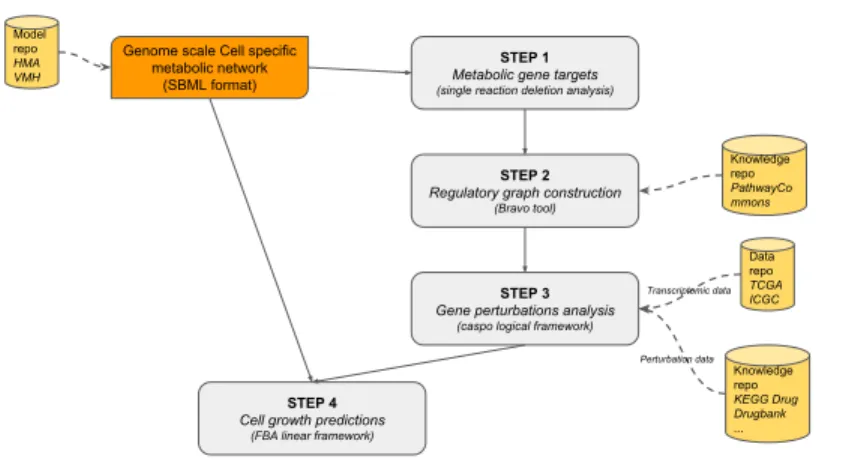
There now exists in the literature a huge amount of descriptions of gene perturba-tions induced by changes in the environment, drug effect and diseases [17]. We aim here at studying, at a genome scale level, the effect of such gene perturbations at a metabolic scale. In the past few years, several approaches have been proposed to in-tegrate metabolic network with regulatory informations (see [25]). The challenge re-mains to integrate regulatory informations at a genome scale for both the metabolic network and the regulatory network. We propose a framework that enables such an integration relying on logic programming, linear programming and semantic web technologies. The framework that we propose here is depicted in Fig. 8 and consists in four steps.

One first starts with a fully functional reconstructed metabolic network that al-lows to simulate the biological pathway of interest. Such metabolic networks can be downloaded from different model repositories like BiGG database [18], Virtual Metabolic Human [8], or Human Metabolic Atlas [36] for instance.

Step 1 of the framework consists in performing a single reaction deletion analysis that allows to decipher which reactions have an impact on the cell growth. We next consider all the proteins that influence these reactions and finally, the genes that regulate these proteins. These informations are sometimes available in the SBML

Genome scale Cell specific metabolic network (SBML format) Model repo HMA VMH STEP 1

Metabolic gene targets

(single reaction deletion analysis)

STEP 2

Regulatory graph construction

(Bravo tool) Knowledge repo PathwayCo mmons STEP 3

Gene perturbations analysis

(caspo logical framework)

Data repo TCGA ICGC Knowledge repo KEGG Drug Drugbank ... Transcriptomic data Perturbation data STEP 4

Cell growth predictions

(FBA linear framework)

Fig. 8 A hybrid framework to study drug induced gene perturbations at a metabolic scale.

file that encodes the metabolic network. If not, it is very often possible to retrieve these correspondences by querying the literature in an appropriate way. At the end,

it defines the setT of target genes. Notice that this step has an important role in the

study since it drastically reduces the size of the considered problem.

Step 2 consists in reconstructing the upstream regulation network by using a tool we have recently developed, Bravo [22], which uses semantic web technologies to query the Pathway Commons database in order to obtain all the known regulators of a given set of genes. This operation is performed in an iterative way ensuring a completeness of the reconstructed graph. At the end, one gets a directed and labeled graph that describes the regulations that can influence the activation of genes in set T . This latter graph can be used as a Prior Knowledge Network for either coloring approaches similar to what was described in Section 2.1 such as IGGY [41] or for the caspo framework (see Section 2.2). The choice of the modeling framework will depend mainly on the number of datasets at hand, as well as on the size of the PKN. Recall that coloring approaches can deal with more uncertainty and PKNs of thou-sands of components, while caspo approaches can deal with middle-scale PKNs. On the other hand, caspo approaches are more specific, because of the Boolean modeling; while coloring approaches, propose several coloring models, and rather prediction distributions across different patients (see Fig 3).

In Step 3, one uses the chosen modeling framework to obtain computational

pre-dictions on the activities of the targeted genes inI . Notice that the experimental

observations for this step will come from publicly available transcriptomic data and the different conditions of the system arise from knowledge repositories of drug interactions such as DrugBank [47] or KeggDrug [17] for instance.

The final step consists in predicting the growth rate while taking into account the predicted activities of the targeted genes. Here, one applies Flux Balance Analysis techniques. There, the blocked reactions in the model are deduced by the predicted activities of targeted genes obtained in Step 3. Notice that, if the chosen modeling

framework did not provide a certain prediction, and thus a single assignment of gene activities, the obtained predicted growth rates values are not unique too.

5 Conclusion

We have presented on-going and recently published works destined to elucidate computational models from patients datasets. Our goal, in all the previously pre-sented approaches, is to make sense from a mechanistic perspective of the underly-ing differences among different classes of patients. Rather than usunderly-ing statistical and machine learning methods applied only to the experimental proteomics or transcrip-tomic datasets, we have included a general Prior Knowledge Network, component by using publicly available repositories. This PKN dimension allowed our meth-ods to propose specific (to patient class or cell line) mechanisms relating molecular species, as subgraphs or Boolean models. We believe that this mechanistic infor-mation is a powerful predictors of disease, complementary and comparable to bio-clinical markers as we could proof in [29] for Myelome Multiple patients. All of the proposed methods are based on logic programming, mainly on Answer Set Pro-gramming. These methods are publicly available and we have referenced through out this chapter the git repositories where the related softwares are available.

In complement to this we describe metabolic network systems, analyzed through Linear Programming approaches. We sketched a methodology, based on our pre-viously published methods, that combines logic programming regulatory and sig-naling modeling with linear programming metabolic modeling. This hybrid model represents a more realistic object of study which connects qualitative with quantita-tive predictions and integrate drugs information into computational models to link model predictions with disease response.

Acknowledgments

This work has been partly supported by the SyMeTRIC Pays de la Loire Connect Talent project and by the GRIOTE Pays de la Loire Regional project. We also would like to thank Bertrand Miannay for fruitful discussions.

References

[1] Agren R, Bordel S, Mardinoglu A, Pornputtapong N, Nookaew I, Nielsen J (2012) Recon-struction of genome-scale active metabolic networks for 69 human cell types and 16 cancer types using INIT. PLoS Comput Biol 8(5):e1002,518

[2] Agren R, Mardinoglu A, Asplund A, Kampf C, Uhlen M, Nielsen J (2014) Identification of anticancer drugs for hepatocellular carcinoma through personalized genome-scale metabolic modeling. Mol Syst Biol 10:721

[3] Apic G, Ignjatovic T, Boyer S, Russell RB (2005) Illuminating drug discovery with biological pathways. FEBS Lett 579(8):1872–1877

[4] Ates O (2015) Systems Biology of Microbial Exopolysaccharides Production. Frontiers in bioengineering and biotechnology 3:200

[5] Baral C (2003) Knowledge Representation, Reasoning and Declarative Problem Solving. Cambridge University Press

[6] Bentele M, Lavrik I, Ulrich M, St¨oßer S, Heermann D, Kalthoff H, Krammer P, Eils R (2004) Mathematical modeling reveals threshold mechanism in CD95-induced apoptosis. The Jour-nal of Cell Biology 166(6)

[7] Bordbar A, Monk JM, King ZA, Palsson BO (2014) Constraint-based models predict metabolic and associated cellular functions. Nature Reviews Genetics 15(2):107–120 [8] Brunk E, Sahoo S, Zielinski DC, Altunkaya A, Drager A, Mih N, Gatto F, Nilsson A,

Pre-ciat Gonzalez GA, Aurich MK, Prli A, Sastry A, Danielsdottir AD, Heinken A, Noronha A, Rose PW, Burley SK, Fleming RMT, Nielsen J, Thiele I, Palsson BO (2018) Recon3D enables a three-dimensional view of gene variation in human metabolism. Nat Biotechnol 36(3):272–281

[9] Chebouba L, Miannay B, Boughaci D, Guziolowski C (2018) Discriminate the response of Acute Myeloid Leukemia patients to treatment by using proteomics data and Answer Set Programming. BMC Bioinformatics 19(Suppl 2):59

[10] Fabregat A, Jupe S, Matthews L, Sidiropoulos K, Gillespie M, Garapati P, Haw R, Jassal B, Korninger F, May B, Milacic M, Roca CD, Rothfels K, Sevilla C, Shamovsky V, Shorser S, Varusai T, Viteri G, Weiser J, Wu G, Stein L, Hermjakob H, D’Eustachio P (2018) The Reactome Pathway Knowledgebase. Nucleic Acids Res 46(D1):D649–D655

[11] Gatto F, Miess H, Schulze A, Nielsen J (2015) Flux balance analysis predicts essential genes in clear cell renal cell carcinoma metabolism. Sci Rep 5:10,738

[12] Gawehn E, Hiss JA, Schneider G (2016) Deep learning in drug discovery. Molecular Infor-matics 35(1):3–14

[13] Han H, Cho JW, Lee S, Yun A, Kim H, Bae D, Yang S, Kim CY, Lee M, Kim E, Lee S, Kang B, Jeong D, Kim Y, Jeon HN, Jung H, Nam S, Chung M, Kim JH, Lee I (2018) TRRUST v2: an expanded reference database of human and mouse transcriptional regulatory interactions. Nucleic Acids Res 46(D1):D380–D386

[14] Han H, Cho JW, Lee S, Yun A, Kim H, Bae D, Yang S, Kim CY, Lee M, Kim E, Lee S, Kang B, Jeong D, Kim Y, Jeon HN, Jung H, Nam S, Chung M, Kim JH, Lee I (2018) TRRUST v2: an expanded reference database of human and mouse transcriptional regulatory interactions. Nucleic Acids Res 46(D1):D380–D386

[15] Hill SM, Heiser LM, Cokelaer T, Unger M, Nesser NK, Carlin DE, Zhang Y, Sokolov A, Paull EO, Wong CK, et al (2016) Inferring causal molecular networks: empirical assessment through a community-based effort. Nature methods 13(4):310–318

[16] Hill SM, Nesser NK, Johnson-Camacho K, Jeffress M, Johnson A, Boniface C, Spencer SE, Lu Y, Heiser LM, Lawrence Y, et al (2017) Context specificity in causal signaling networks revealed by phosphoprotein profiling. Cell systems 4(1):73–83

[17] Kanehisa M, Araki M, Goto S, Hattori M, Hirakawa M, Itoh M, Katayama T, Kawashima S, Okuda S, Tokimatsu T, Yamanishi Y (2008) KEGG for linking genomes to life and the environment. Nucleic Acids Res 36(Database issue):D480–484

[18] King ZA, Lu J, Drager A, Miller P, Federowicz S, Lerman JA, Ebrahim A, Palsson BO, Lewis NE (2016) BiGG Models: A platform for integrating, standardizing and sharing genome-scale models. Nucleic Acids Res 44(D1):D515–522

[19] Korkut A, Wang W, Demir E, Aksoy BA, Jing X, Molinelli EJ, Babur O, Bemis DL, Onur Sumer S, Solit DB, Pratilas CA, Sander C (2015) Perturbation biology nominates upstream-downstream drug combinations in RAF inhibitor resistant melanoma cells. Elife 4

[20] Kuhn M, Yates P, Hyde C (2016) Statistical Methods for Drug Discovery, Springer Interna-tional Publishing, Cham, pp 53–81

[21] Le Jeune P, Paris J, Voinea J, Liu J, Boulkenafet K (2018) Iguana. https://github.com/ipeter50/Iguana

[22] Lefebvre M, Bourdon J, Guziolowski C, Gaignard A (2017) Regulatory and signaling net-work assembly through linked open data. demo paper, Journ´ees Ouvertes en Biologie, Infor-matique et Math´eInfor-matiques (JOBIM2017)

[23] Lima AN, Philot EA, Trossini GHG, Scott LPB, Maltarollo VG, Honorio KM (2016) Use of machine learning approaches for novel drug discovery. Expert Opinion on Drug Discovery 11(3):225–239

[24] Liu W, Li C, Xu Y, Yang H, Yao Q, Han J, Shang D, Zhang C, Su F, Li X, Xiao Y, Zhang F, Dai M, Li X (2013) Topologically inferring risk-active pathways toward precise cancer classification by directed random walk. Bioinformatics (Oxford, England) 29(17):2169–77, DOI 10.1093/bioinformatics/btt373

[25] Machado D, Herrgard M (2014) Systematic evaluation of methods for integration of transcriptomic data into constraint-based models of metabolism. PLoS Comput Biol 10(4):e1003,580

[26] Magnusdottir S, Heinken A, Kutt L, Ravcheev DA, Bauer E, Noronha A, Greenhalgh K, Jager C, Baginska J, Wilmes P, Fleming RM, Thiele I (2017) Generation of genome-scale metabolic reconstructions for 773 members of the human gut microbiota. Nat Biotechnol 35(1):81–89

[27] Marx V (2013) Biology: The big challenges of big data. Nature 498(7453):255–260, DOI 10.1038/498255a

[28] Miannay B (2017) Iggy-POC. https://github.com/BertrandMiannay/Iggy-POC

[29] Miannay B, Minvielle S, Roux O, Drouin P, Avet-Loiseau H, Gu´erin-Charbonnel C, Gouraud W, Attal M, Facon T, Munshi NC, Moreau P, Campion L, Magrangeas F, Guziolowski C (2017) Logic programming reveals alteration of key transcription factors in multiple myeloma. Scientific Reports 7(1):9257

[30] Miannay B, Minvielle S, Magrangeas F, Guziolowski C (2018) Constraints on signaling net-work logic reveal functional subgraphs on Multiple Myeloma OMIC data. BMC Syst Biol 12(Suppl 3):32

[31] Mitra K, Carvunis AR, Ramesh SK, Ideker T (2013) Integrative approaches for finding mod-ular structure in biological networks. Nat Rev Genet 14(10):719–732

[32] Murphy RF (2011) An active role for machine learning in drug development. Nat Chem Biol 7:327–330

[33] Nevins JR (2001) The Rb/E2F pathway and cancer. Human molecular genetics 10(7):699– 703, DOI 10.1093/hmg/10.7.699

[34] Noren D, Long B, Norel R, Rrhissorrakrai K, Hess K, Hu C, Bisberg A, Schultz A, Engquist E, Liu L, Lin X, Chen G, Xie H, Hunter G, Boutros P, Stepanov O, Norman T, Friend S, Stolovitzky G, Kornblau S, Qutub A, DREAM 9 AML-OPC Consortium (2016) A crowd-sourcing approach to developing and assessing prediction algorithms for aml prognosis. PLoS Computational Biology 12(6)

[35] Ostrowski M, Paulev´e L, Schaub T, Siegel A, Guziolowski C (2016) Boolean network iden-tification from perturbation time series data combining dynamics abstraction and logic pro-gramming. Biosystems 149:139–153

[36] Pornputtapong N, Nookaew I, Nielsen J (2015) Human metabolic atlas: an online resource for human metabolism. Database (Oxford) 2015:bav068

[37] Pratt D, Chen J, Pillich R, Rynkov V, Gary A, Demchak B, Ideker T (2017) NDEx 2.0: A Clearinghouse for Research on Cancer Pathways. Cancer Res 77(21):e58–e61

[38] Rajkumar SV (2016) Multiple myeloma: 2016 update on diagnosis, risk-stratification, and management. American Journal of Hematology 91(7):719–734, DOI 10.1002/ajh.24402 [39] Razzaq M, Paulev´e L, Ostrowski M (2018) Caspo-ts. https://github.com/misbahch6/caspo-ts

[40] Schaefer CF, Anthony K, Krupa S, Buchoff J, Day M, Hannay T, Buetow KH (2009) PID: the Pathway Interaction Database. Nucleic acids research 37(Database issue):D674–9, DOI 10.1093/nar/gkn653

[41] Thiele S, Cerone L, Saez-Rodriguez J, Siegel A, Guzioowski C, Klamt S (2015) Extended notions of sign consistency to relate experimental data to signaling and regulatory network topologies. BMC bioinformatics 16(1):345, DOI 10.1186/s12859-015-0733-7

[42] Thomas D, Powell JA, Vergez F, Segal DH, Nguyen NY, Baker A, Teh TC, Barry EF, Sarry JE, Lee EM, Nero TL, Jabbour AM, Pomilio G, Green BD, Manenti S, Glaser SP, Parker MW, Lopez AF, Ekert PG, Lock RB, Huang DC, Nilsson SK, Recher C, Wei AH, Guthridge MA (2013) Targeting acute myeloid leukemia by dual inhibition of PI3K signaling and Cdk9-mediated Mcl-1 transcription. Blood 122(5):738–748

[43] Thomas PD, Kejariwal A, Campbell MJ, Mi H, Diemer K, Guo N, Ladunga I, Ulitsky-Lazareva B, Muruganujan A, Rabkin S, Vandergriff JA, Doremieux O (2003) PANTHER: a browsable database of gene products organized by biological function, using curated pro-tein family and subfamily classification. Nucleic Acids Res 31(1):334–341

[44] Videla S, Guziolowski C, Eduati F, Thiele S, Grabe N, Saez-Rodriguez J, Siegel A (2012) Revisiting the training of logic models of protein signaling networks with asp. In: Computa-tional Methods in Systems Biology, Springer Berlin/Heidelberg, pp 342–361

[45] Videla S, Saez-Rodriguez J, Guziolowski C, Siegel A (2017) caspo: a toolbox for automated reasoning on the response of logical signaling networks families. Bioinformatics 33(6):947– 950

[46] Wang, Yuanyuan (Marcia) (2005) Statistical methods for high throughput screening drug discovery data. PhD thesis, URL http://hdl.handle.net/10012/1204

[47] Wishart DS, Feunang YD, Guo AC, Lo EJ, Marcu A, Grant JR, Sajed T, Johnson D, Li C, Sayeeda Z, Assempour N, Iynkkaran I, Liu Y, Maciejewski A, Gale N, Wilson A, Chin L, Cummings R, Le D, Pon A, Knox C, Wilson M (2018) DrugBank 5.0: a major update to the DrugBank database for 2018. Nucleic Acids Res 46(D1):D1074–D1082