HAL Id: tel-01693270
https://tel.archives-ouvertes.fr/tel-01693270
Submitted on 26 Jan 2018
HAL is a multi-disciplinary open access
archive for the deposit and dissemination of sci-entific research documents, whether they are pub-lished or not. The documents may come from teaching and research institutions in France or abroad, or from public or private research centers.
L’archive ouverte pluridisciplinaire HAL, est destinée au dépôt et à la diffusion de documents scientifiques de niveau recherche, publiés ou non, émanant des établissements d’enseignement et de recherche français ou étrangers, des laboratoires publics ou privés.
Florent Bocquelet
To cite this version:
Florent Bocquelet. Toward a brain-computer interface for speech restoration. Electronics. Université Grenoble Alpes, 2017. English. �NNT : 2017GREAS008�. �tel-01693270�
THÈSE
Pour obtenir le grade de
DOCTEUR DE LA COMMUNAUTE UNIVERSITE
GRENOBLE ALPES
Spécialité : Biotechnologie, Instrumentation, Signal Arrêté ministériel : 25 mai 2016
Présentée par
Florent BOCQUELET
Thèse dirigée par Blaise YVERT, Directeur de recherche,
INSERM, et
codirigée par Laurent GIRIN, Professeur des Universités,
Université Grenoble Alpes
préparée au sein des laboratoires BrainTech et Gipsa-lab
dans l'École Doctorale Ingénierie pour la Santé, la Cognition et
l’Environnement
Vers une interface
cerveau-machine pour la restauration de
la parole
Thèse soutenue publiquement le 24 avril 2017, devant le jury composé de :
M. Stéphan CHABARDES
Professeur (CHUG), Membre
M. Frank GUENTHER
Professeur (Université de Boston), Rapporteur
M. Thomas HUEBER
Chargé de recherche (CNRS), Membre
M. Oliver MÜLLER
Professeur (Université de Freiburg), Membre
Mme. Tanja SCHULTZ
Professeur (Université de Brême), Rapportrice
Mme. Agnès TREBUCHON
Abstract
Restoring natural speech in paralyzed and aphasic people could be achieved using a brain-computer interface controlling a speech synthesizer in real-time. The aim of this thesis was thus to develop three main steps toward such proof of concept.
First, a prerequisite was to develop a speech synthesizer producing intelligible speech in real-time with a reasonable number of control parameters. Here we chose to synthesize speech from movements of the speech articulators since recent studies suggested that neural activity from the speech motor cortex contains relevant information to decode speech, and especially articulatory features of speech. We thus developed a speech synthesizer that produced intelligible speech from articulatory data. This was achieved by first recording a large dataset of synchronous articulatory and acoustic data in a single speaker. Then, we used machine learning techniques, especially deep neural networks, to build a model able to convert articulatory da ta into speech. This synthesizer was built to run in real time. Finally, as a first step toward future brain control of this synthesizer, we tested that it could be controlled in real-time by several speakers to produce intelligible speech from articulatory movements in a closed-loop paradigm.
Second, we investigated the feasibility of decoding speech and articulatory features from neural activity essentially recorded in the speech motor cortex. We built a tool that allowed to localize active cortical speech areas online during awake brain surgery at the Grenoble Hospital and tested this system in two patients with brain cancer. Results show that the motor cortex exhibits specific activity during speech production in the beta and gamma bands, which are also present during speech imagination. The recorded data could be successfully analyzed to decode speech intention, voicing activity and the trajectories of the main articulators of the vocal tract above chance.
Finally, we addressed ethical issues that arise with the development and use of brain-computer interfaces. We considered three levels of ethical questionings, dealing respectively with the animal, the human being, and the human species.
Résumé
Restorer la faculté de parler chez des personnes paralysées et aphasiques pourrait être envisagée via
l’utilisation d’une interface cerveau-machine permettant de contrôler un synthétiseur de parole en temps réel. L’objectif de cette thèse était de développer trois aspects nécessaires à la mise au point d’une telle preuve de
concept.
Premièrement, un synthétiseur permettant de produire en temps-réel de la parole intelligible et controlé par un nombre raisonable de paramètres est nécessaire. Nous avons choisi de synthétiser de la parole à partir des mouvements des articulateurs du conduit vocal. En effet, des études récentes ont suggéré que l’activité neuronale du cortex moteur de la parole pourrait contenir suffisamment d’information pour décoder la parole, et particulièrement ses propriété articulatoire (ex. l’ouverture des lèvres). Nous avons donc développé un
synthétiseur produisant de la parole intelligible à partir de données articulatoires. Dans un premier temps, nous avons enregistré un large corpus de données articulatoire et acoustiques synchrones chez un locuteur. Ensuite,
nous avons utilisé des techniques d’apprentissage automatique, en particulier des réseaux de neurones profonds,
pour construire un modèle permettant de convertir des données articulatoires en parole. Ce synthétisuer a été construit pour fonctionner en temps réel. Enfin, comme première étape vers un contrôle neuronal de ce
synthétiseur, nous avons testé qu’il pouvait être contrôlé en temps réel par plusieurs locuteurs, pour produire de
la parole inetlligible à partir de leurs mouvements articulatoires dans un paradigme de boucle fermée.
Deuxièmement, nous avons étudié le décodage de la parole et de ses propriétés articulatoires à partir
d’activités neuronales essentiellement enregistrées dans le cortex moteur de la parole. Nous avons construit un outil permettant de localiser les aires corticales actives, en ligne pendant des chirurgies éveillées à l’hôpital de Grenoble, et nous avons testé ce système chez deux patients atteints d’un cancer du cerveau. Les résultats ont
montré que le cortex moteur exhibe une activité spécifique pendant la production de parole dans les bandes beta
et gamma du signal, y compris lors de l’imagination de la parole. Les données enregistrées ont ensuite pu être analysées pour décoder l’intention de parler du sujet (réelle ou imaginée), ainsi que la vibration des cordes
vocales et les trajectoires des articulateurs principaux du conduit vocal significativement au dessus du niveau de la chance.
Enfin, nous nous sommes intéressés aux questions éthiques qui accompagnent le développement et l’usage des interfaces cerveau-machine. Nous avons en particulier considéré trois niveaux de réflexion éthique concernant
Content
Abstract ... 2 Résumé ... 2 Acknowledgement ... 3 Content ... 4 List of figures ... 12 List of tables ... 22Acronyms and terms... 23
Phonetic notation ... 24
Introduction ... 25
Motivation of research ... 25
Organization of the manuscript ... 26
Part 1: State of the art... 28
Chapter 1: Brain-computer interfaces for speech rehabilitation ... 28
I. Introduction: Brain-computer interfaces for communication ... 28
1. Neural activity recording ... 29
2. Metabolic signals recording ... 32
a. Functional magnetic resonance imaging ... 32
b. Functional near-infrared spectroscopy ... 33
c. Optical imaging of intrinsic signals ... 33
d. Positron emission tomography ... 33
3. Electrophysiological signals recording ... 34
a. Electroencephalography ... 34
b. Magnetoencephalography ... 35
c. Electrocorticography ... 35
d. Micro-electrocorticography ... 36
e. Stereo-electroencephalography ... 36
f. Intracortical micro-electrodes arrays ... 36
II. Cortical speech production areas ... 37
1. Speech areas ... 37
2. Speech production ... 38
a. Overt speech ... 38
5
2. Continuous decoding ... 42
IV. Conclusion ... 43
1. Choice of a recording technique to monitor speech brain signals ... 43
2. Choice of a brain region ... 44
3. Choice of a decoding and synthesis approach ... 45
Chapter 2: Articulatory-based speech synthesis ... 47
I. Introduction ... 47
1. Speech production ... 47
2. Speech synthesis ... 48
II. Formant synthesis ... 49
III. Text-to-speech synthesis ... 49
1. Concatenative synthesis ... 49
2. Statistical parametric synthesis ... 50
IV. Articulatory-based speech synthesis ... 50
1. Methods for articulatory data acquisition ... 51
a. X-ray imaging ... 51
b. Magnetic Resonance Imaging ... 52
c. Video recording ... 52
d. Ultrasonography ... 52
e. Electromyography ... 53
f. Electropalatography ... 54
g. Electromagnetic articulography ... 55
h. Choice of an articulatory data recording method ... 56
2. Physical modeling of the vocal tract ... 57
a. Modeling the geometry of oral cavities ... 57
i. 2D and 3D models of oral cavities ... 58
ii. Geometrical, statistical and biomechanical models of oral cavities ... 58
b. Modeling the acoustic properties of oral cavities ... 58
3. Non-physical articulatory-based synthesis ... 59
a. Discrete approaches ... 60
b. Continuous approaches ... 60
V. GMM-based articulatory-to-acoustic mapping ... 62
6
2. Training algorithm for the trajectory GMM ... 64
VI. DNN-based articulatory-to-acoustic mapping ... 65
1. Artificial Neural Network ... 65
2. Training artificial neural networks ... 66
3. Difficulties when training deep neural networks ... 68
VII. Conclusion ... 69
Part 2: Goal of the thesis ... 70
Part 3: Thesis result 1 – Articulatory-based speech synthesis for BCI applications ... 72
Chapter 3: The BY2014 articulatory-acoustic corpus ... 73
I. Introduction ... 73
II. The PB2007 corpus ... 73
1. Articulatory data acquisition and parametrization for the PB2007 corpus... 73
2. Acoustic data acquisition and parametrization for the PB2007 corpus ... 74
3. Content of the PB2007 corpus ... 75
III. The BY2014 corpus ... 76
1. Articulatory data acquisition and parametrization for the BY2014 corpus .... 76
2. Acoustic data acquisition and parametrization for the BY2014 corpus ... 77
3. Content of the BY2014 corpus ... 77
Chapter 4: Articulatory-based speech synthesis ... 79
I. Introduction ... 79
II. Articulatory-to-acoustic mapping ... 79
1. GMM-based mapping ... 79
a. Choice of GMM hyper-parameters ... 79
b. Implementation details of the trajectory GMM ... 80
2. DNN-based mapping ... 80
a. Proposed approach for training DNNs for regression ... 81
b. Choice of DNN hyper-parameters ... 82
c. Implementation details of the DNNs ... 85
3. Articulatory-to-acoustic mapping and speech synthesis ... 89
a. Synthesis for the PB2007 corpus ... 89
b. Synthesis for the BY2014 corpus ... 90
III. Artificial degradation of the articulatory data ... 91
7
b. Deep Auto-Encoder ... 93
IV. Evaluation of the speech synthesis intelligibility ... 94
1. Objective evaluation based on automatic speech recognition ... 94
2. Subjective evaluation using listening tests ... 96
a. Evaluation on the PB2007 corpus ... 96
b. Evaluation on the BY2014 corpus ... 97
3. Statistical analysis ... 98
a. Statistical analysis for the PB2007 synthesis ... 98
b. Statistical analysis for the BY2014 synthesis ... 98
V. Results ... 99
1. Convergence of the proposed approach for training DNNs for regression .... 99
2. PB2007 corpus ... 99
a. Influence of GMM hyper-parameters ... 99
b. Influence of DNN hyper-parameters ... 100
c. Comparison of GMM and DNN ... 101
d. Speech synthesis from reduced articulatory data ... 102
e. Speech synthesis from noisy articulatory data ... 102
f. Conclusion on the PB2007 synthesis ... 103
3. BY2014 corpus ... 104
a. Evaluation results on vowels and VCVs ... 104
b. Evaluation results on full sentences ... 107
c. Conclusion on the BY2014 synthesis ... 108
VI. Conclusion on the articulatory-based speech synthesis ... 109
Chapter 5: Real-time control of an articulatory-based speech synthesizer for silent speech conversion ... 111
I. Introduction ... 111
II. Methods ... 112
1. Subjects and experimental design of the real-time closed-loop synthesis .... 112
2. Articulatory-to-articulatory mapping ... 114
3. Implementation details ... 115
4. Closed-loop experimental paradigm ... 115
5. Evaluation of the synthesis quality ... 116
8
III. Results ... 117
1. Accuracy of the articulatory-to-articulatory mapping ... 117
2. Intelligibility of the real-time closed-loop synthesis ... 119
3. Spontaneous conversations ... 122
IV. Conclusion on the real-time control of the articulatory-based speech synthesizer 122 Discussion on the articulatory-based speech synthesis for BCI applications ... 124
Part 4: Thesis result 2 – Toward a BCI for speech rehabilitation ... 126
Chapter 6: Per-operative mapping of speech-related brain activity ... 127
I. Introduction ... 127
II. Methods ... 128
1. Subjects and experimental design ... 128
a. First patient ... 128
b. Second patient ... 130
2. Automatic speech detection ... 131
3. Extraction of speech-related brain activity ... 134
4. Mapping of speech-related brain activity ... 136
5. Coregistration of the electrodes on the operative field ... 138
6. Coregistration of the electrodes on the reconstructed cortical surface ... 140
7. Implementation details ... 142
III. Results ... 143
1. ClientMap: a neural activity mapping software dedicated to speech ... 143
a. Parameters panel ... 144 b. Spectrum panel ... 145 c. Score panel ... 145 d. Features panel ... 146 e. Electrode panel ... 146 f. Maps panel ... 146
g. Raw data panel ... 147
2. Mapping of speech-related brain activity ... 147
a. First patient ... 147
i. Overt speech ... 147
9
Chapter 7: Speech decoding from neural activity ... 154
I. Introduction ... 154
II. Methods ... 154
1. Decoding of speech intention ... 154
a. Subjects and experimental design ... 155
b. Features extraction ... 155
i. First patient ... 155
ii. Second patient ... 155
c. Classification method ... 156
d. Evaluation of the speech state decoding ... 157
2. Decoding of the voicing activity ... 158
a. Subjects, experimental design and features extraction ... 158
b. Classification method and results evaluation ... 158
3. Decoding of articulatory features ... 158
a. Subjects and experimental design ... 158
b. Neural features pre-selection and extraction ... 159
c. Estimation of articulatory features ... 159
d. Neural-to-articulatory mapping... 160
e. Evaluation of the decoding ... 161
4. Decoding of acoustic features ... 161
a. Neural-to-acoustic mapping ... 161
b. Comparison with the neural-to-articulatory mapping ... 161
III. Results ... 163
1. Decoding of speech intention ... 163
a. First patient ... 163
i. Decoding overt speech intervals ... 163
ii. Decoding covert speech intervals ... 164
b. Second patient ... 164
2. Decoding of the voicing activity ... 165
3. Decoding of articulatory features ... 166
4. Decoding of acoustic features ... 171
5. Comparison of the neural-to-articulatory and neural-to-acoustic mappings 176 IV. Conclusion on the speech decoding from neural activity ... 178
10
II. The animal ... 183
1. The fight against pain, suffering and anxiety in animals ... 183
2. Animals are not things ... 183
III. The human being ... 184
1. Addressing the aroused hope ... 184
2. Risk/benefits ratio ... 185
3. Informed consent and patient’s involvement ... 185
4. Accessibility of BCIs ... 186
5. Modulating the brain activity with BCIs: what consequences? ... 186
6. Reliability and safety of BCIs ... 186
7. Responsibility when using BCIs ... 187
IV. The human species ... 187
1. BCIs as future means of enhancement? ... 188
2. The risk of transhumanism? ... 188
3. Freedom and BCI ... 189
V. Conclusion ... 190
Part 6: Conclusions and Perspectives ... 191
Main contributions and results ... 191
Perspectives ... 194
Annexes ... 197
Annex 1: List of sentences for the evaluation of the reference offline synthesis. 197 Annex 2: List of sentences from the spontaneous conversation during the real-time control of the synthesizer ... 198
Bibliography ... 199 Publications ... 222 Journal articles ... 222 Book chapters ... 222 International conferences ... 222 Résumé en français... 223 I. Introduction ... 223
II. Résumé de l’état de l’art ... 224
1. Interfaces cerveau-machine pour la restauration de la parole ... 224
11
III. Synthèse de parole à partir de données articulatoires ... 227
1. Enregistrement d’un corpus articulatoire-acoustique ... 227
2. Synthèse de parole à partir de données articulatoires ... 227
3. Contrôle temps-réel du synthétiseur à partir de parole silencieuse ... 228
IV. Vers une interface cerveau-machine pour la restauration de la parole ... 229
1. Cartographie peropératoire des aires corticales de la parole ... 229
2. Décodage de la parole à partir de l’activité corticale ... 230
V. Questions éthiques relatives aux interfaces cerveau-machine ... 231
List of figures
Fig. 1: Principle of a speech brain-computer interface. Neural activity is recorded from
various speech-related brain areas and then processed to extract informative features, which are then decoded into control parameters for a speech synthesizer. The synthesis is performed in real-time so that the subject can benefit from the auditory feedback to better control the synthesizer. ... 29
Fig. 2: Structure of a neuron. A neuron is composed by dendrites, the cell body and an
axon that ends by synapses that contact other neurons. The transmission of action potentials at the synapses is generally chemical, by releasing neurotransmitters. Source: thatsbasicscience.blogspot.fr ... 30
Fig. 3: Action potential. Left – An action potential is a short peak signal, that can be
described by 4 phases: rest (1), depolarisation (2), repolarisation (3) and refractory period until rest (4). Right – The 4 phases of the action potential are generated by succesive activations and deactivations of ionic channels (green: Na+/K+ pump, light yellow: voltage-gated Na+ channel, orange: Voltage-gated K+ channel). Source: www.vce.bioninja.com.au. ... 31
Fig. 4: MEG, EEG, ECoG, µECoG, SEEG and MEA recordings. With MEG, magnetic
sensors are placed all around the head. In EEG, relatively large electrodes are placed over the scalp. In ECoG, smaller electrodes are placed under the skull, either above (epidural) or under (subdural) the dura mater. µECoG is similar to ECoG but uses very high density grids with smaller electrodes. SEEG are thin wires on which are spaced several electrodes that penetrates the brain in depth. MEA consists of micro-electrodes penetrating the cortex. Adapted from (Jorfi et al., 2015). ... 34
Fig. 5: Spatial organization of the vSMC during speech production. Left – Location of
the ECoG grid electrodes over the vSMC. Middle – Functional somatotopic organization of speech-articulator representations in vSMC plotted with regard to the anteroposterior (AP) distance from the central sulcus and dorsoventral (DV) distance from the Sylvian fissure. Lips (L, red); jaw (J, green); tongue (T, blue); larynx (X, black); mixed (yellow). Right – Hierarchical clustering of the cortical activities for consonants (left) and vowels (right), with branches labeled with linguistic categories. (Bouchard et al., 2013). ... 39
Fig. 6: Anatomy of the vocal tract and its configuration for different phonemes. Left
– the main speech articulators are the tongue, the lips; the soft palate, the larynx and the teeth (Bluetree Publishing ©2013). Right – Different vocal tract configuration are shown, for /d/, /g/, /a/, /i/ and /u/ (www.indiana.edu). ... 47
Fig. 7: Kratzenstein's resonators shapes and the Voder. Left – each vocal tract shape
produces a different vowel when air is blown through them (Schroeder, 1993). Right – The Voder is controlled through a keyboard and some wrist controls. ... 48
Fig. 8: Vocal tract shape extraction from X-ray cineradiography. The red, yellow and
green marks show the manually extracted vocal tract shapes. Source: XArticulator software by Yves Laprie (https://members.loria.fr/YLaprie/ACS/index.htm). ... 51
Fig. 9: vocal tract shape extraction from MRI. Left – image obtained by MRI, and
automatically extracted shape (green line with white dots). Source:
www.cmiss.bioeng.auckland.ac.nz. Right – 3D printed vocal tracts using three dimensional MRI data. Source: www.speech.math.aalto.fi ... 52
13
... 53
Fig. 11: Articulatory data from EMG. Here, an EMG array was placed to record cheek
muscles activation (Wand et al., 2013). ... 54
Fig. 12: Artificial palate for electropalatography. Each metal disk is an electrode that
allows to detect contacts of the tongue with the palate. Source: www.articulateinstruments.com. ... 54
Fig. 13: Electromagnetic articulography. EMA coils are glued to the lips, the jaw, the
tongue and the soft palate (Bocquelet et al., 2016a). ... 55
Fig. 14: Conventional unit of an artificial neural network. The unit has one output, and
several inputs Input1, …, InputN each one with an associated weight Weight1, …, WeightN. A unit is defined by its activation function σ and its bias, so that the output of the unit is the application of σ to the weighted sum of its inputs, to which is added the bias. ... 65
Fig. 15: Feed-forward neural network. Units are organized into layers. All units of a
layer are connected to all units of the next layer. ... 66
Fig. 16: PB2007 articulatory and acoustic data. A – Positioning of the sensors on the
upper lip (1), lower lip (2), tongue tip (3), tongue dorsum (4), and tongue back (5). The jaw sensor was glued at the base of the incisive (not visible in this image). B – Articulatory signals and corresponding audio signal for the sentence “Annie s’ennuie loin de mes parents” (“Annie gets bored away from my parents”). For each sensor, the horizontal caudo-rostral X and below the vertical ventro-dorsal Y coordinates projected in the midsagittal plane are plotted. Dashed lines show the phone segmentation obtained by forced-alignment. C – Acoustic features (20 mel-cepstrum coefficients - MEL) and corresponding segmented audio signal for the same sentence as in B. ... 74
Fig. 17: PB2007 articulatory-acoustic database description. A – Occurrence histogram
of all phones of the articulatory-acoustic database. Each bar shows the number of occurrence of a specific phone in the whole corpus. B – Spatial distribution of all articulatory data points of the database (silences excluded) in the midsagittal plane. The positions of the different sensors are plotted with different colors. The labeled positions correspond to the mean position for the 7 main French vowels. ... 75
Fig. 18: BY2014 articulatory and acoustic data. A – Positioning of the sensors on the lip
corners (1 & 3), upper lip (2), lower lip (4), tongue tip (5), tongue dorsum (6), tongue back (7) and velum (8). The jaw sensor was glued at the base of the incisive (not visible in this image). B – Articulatory signals and corresponding audio signal for the sentence “Annie s’ennuie loin de mes parents” (“Annie gets bored away from my parents”). For each sensor, the horizontal caudo-rostral X and below the vertical ventro-dorsal Y coordinates projected in the midsagittal plane are plotted. Dashed lines show the phone segmentation obtained by forced-alignment. C – Acoustic features (25 mel-cepstrum coefficients - MEL) and corresponding segmented audio signal for the same sentence as in B. ... 77
Fig. 19: BY2014 articulatory-acoustic database description. A – Occurrence histogram
of all phones of the articulatory-acoustic database. Each bar shows the number of occurrence of a specific phone in the whole corpus. B – Spatial distribution of all articulatory data points of the database (silences excluded) in the midsagittal plane. The positions of the different sensors (except corner lips) are plotted with different colors. The labeled positions correspond to the mean position for the 7 main French vowels. ... 78
14
output layer, connected to the h1 layer. This initial network was randomly initialized then fine-tuned using the conjugate gradient algorithm. B – The temporary output layer was then deleted. C - The next layer was then added so that the new network was now composed by the input layer h0, the first two hidden layers h1 and h2, and a new temporary output layer, connected to the h2 layer. The weights from the input layer h0 to the fist hidden layer h1 were those obtained at the previous step and the other weights were randomly initialized. The conjugate gradient algorithm was then applied to this network for fine-tuning. D – The temporary output layer was then deleted. E - This process was repeated until all the hidden layers were added. ... 82
Fig. 21: Activation functions of the neural network. A – Logistic sigmoid function. B –
Rectified linear function. ... 83
Fig. 22: DeepSoft – screenshot of the “Dataset” panel. Synchronous input (left) and
ouput (right) data can be loaded from different file formats. ... 86
Fig. 23: DeepSoft – screenshot of the “Preprocessing” panel. Input (left) and output
(right) data can be pre-processed by chaining different pre-processing blocs. For instance here, the output is first z-scored (top-right bloc titled “normalize”). ... 86
Fig. 24: DeepSoft – screenshot of the “Learning data” panel. This panel allows to split
the data into training, test and validation tests, for instance to perform cros-validation. ... 87
Fig. 25: DeepSoft – screenshot of the “Network” panel. The neural network is built by
stacking layers. Here you can see that a linear layer is stacked over a point-wise function layer consisting of 50 hyperbolic units. ... 87
Fig. 26: DeepSoft – screenshot of the “Training” panel. This panel allows to choose and
configure the training algorithm, including regularization methods and criterion function. ... 88
Fig. 27: DeepSoft – screenshot of the “Error” panel. At each epoch, the graph displays
the error on the training set (blue line) and validation set (red line). ... 88
Fig. 28: DeepSoft – screenshot of the “Data” panel. This pannel allows to preview the
network prediction (red line) compared to the ground truth (black line), for each item of the test set (each item is delimited by an alternating white/blue background). ... 89
Fig. 29: Synthesis when using a DNN-based mapping. Using a DNN, articulatory
features are mapped to acoustic features, which are then converted into an audible signal using the MLSA filter and an excitation signal. ... 89
Fig. 30: Inverse glottal filtering. The top-left pannel represents the original audio signal
extracted from an occurrence of the phone /a/. The bottom-left pannel represents the corresponding signal obtained by inverse filtering. The obtained signal is close to a pulse train which period corresponds to the pitch of the original /a/ signal. The left-pannel is a close-up on the first samples of the signal obtained by inverse filtering. ... 90
Fig. 31: Excitation signal generation. First the pitch is extracted from the original audio.
This pitch is then used to generate an excitation signal which is white noise when the pitch is null (i.e. sounds are unvoiced) and a pulse train at the pitch period otherwise (i.e. sounds are voiced). ... 91
Fig. 32: Deep auto-encoder. A deep auto-encoder (DAE) is a symmetric deep neural
network with a “bottle-neck” that is trained to reproduce its input as output. The purpose of the bottle-neck is to force the network to learn a representation of the original data using less parameters, and thus reducing the dimensionality of the original data. A trained DAE can then
15
Fig. 33: Synthesis when using reducted articulatory data. The decoder part of the deep
autoencoder (in blue) is added in front of the articulatory speech synthesizer (in orange) in order to recover full articulatory parameters from reduced parameters. ... 94
Fig. 34: Phoneme sequences alignment. Example of two aligned sequences of phonemes.
S denotes a substitution, D a deletion and I an insertion. ... 96
Fig. 35: Comparison of the conventional neural networks training with our approach.
The graph shows the mean-squared error on the training set for each epoch, when using the conventional training (red line) and our proposed approach (blue line). Vertical dashed blue lines indicate the insertion of a new hidden layer during the pre-training stage. ... 99
Fig. 36: Influence of the GMM hyper-parameters. The thin line shows the phone
recognition according to the number of mixture components in the GMM-based mapping (mean±SD). The thick line represents the recognition accuracy on the anasynth audio... 100
Fig. 37: Influence of the GMM and DNN hyper-parameters. The dashed line shows the
phone recognition according to the number of mixture components in the GMM-based mapping (mean±SD). bar plot shows the phone recognition accuracy according to the number of layers and the number of units per layer using DNN-based mapping (mean±SD). The thick line represents the recognition accuracy on the anasynth audio. ... 100
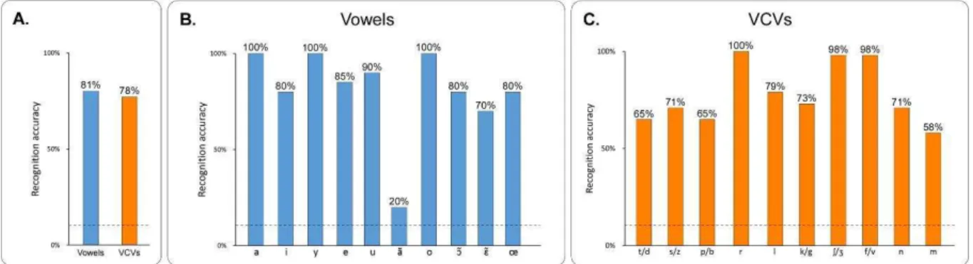
Fig. 38: Recognition accuracy by vowel and consonant for the PB2007 synthesis with a DNN of 3 hidden layers of 100 units each. A – Owerall recognition accuracy for vowel and
VCVs. The dashed line indicates chance level. B – Recognition accuracy by isolated vowel, for the subjective evaluation. The dashed line indicates chance level. Vowels are sorted by number of occurences in the training set, from higher to lower. C – Recognition accuracy according to the middle consonants of the VCVs, for the subjective evaluation. The dashed line indicates chance level. Consonants are sorted by number of occurences in the training set, from higher to lower (for consonant pairs, the sum of occurences of each consonant in the pair was used). 101
Fig. 39: Comparison of GMM and DNN mappings for both objective and subjective evaluations. Each bar corresponds to the recognition accuracy (mean±SD). ... 102 Fig. 40: Evaluation of the PB2007 synthesis with reduced articulatory data. Phone
recognition accuracy (mean±SD) with reduced parameters obtained both by principal component analysis (PCA) and deep auto-encoders (DAE), and with both GMM- and DNN-based mappings. ... 102
Fig. 41: Evaluation of the PB2007 synthesis on noisy articulatory data. Phone
recognition accuracy (mean±SD) on noisy data as a function of the signal to noise ratio (SNR), both for GMM- and DNN-based mappings. ... 103
Fig. 42: Objective and subjective evaluation of the PB2007 synthesis with both noisy and reduced parameters. The bar plot shows the recognition accuracy (mean±SD) based on
objective and subjective evaluations of GMM- and DNN-based mapping on noisy articulatory data (SNR = 10), and on reduced data (DAE with 7 reduced parameters) for the DNN-based mapping. ... 103
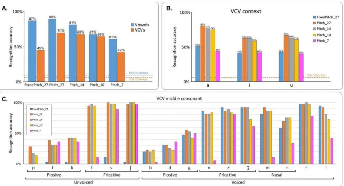
Fig. 43: Subjective evaluation of the intelligibility of the BY2014 speech synthesizer. A – Recognition accuracy for vowels and consonants for each of the 5 synthesis conditions.
The dashed lines show the chance level for vowels (blue) and VCVs (orange). B – Word recognition accuracy for the sentences, in both conditions Pitch_27 and Pitch_14. C –
16
Fig. 44: Confusion matrices of the subjective evaluation of the intelligibility of the BY2014 speech synthesizer. Confusion matrices for vowels (left) and consonants (right), for
each of the three conditions FixedPitch_27, Pitch_27 and Pitch_14. In the matrices, rows correspond to ground truth while columns correspond to user answer. The last column indicates the amount of errors made on each phone. Cells are colored by their values, while text color is for readability only. ... 106
Fig. 45: Subjective evaluation of the intelligibility of the BY2014 speech synthesizer on sentences. Word recognition accuracy for the sentences, for both conditions Pitch_27 and
Pitch_14. ... 107
Fig. 46: Real-time closed loop paradigm. Articulatory data from a silent speaker are
recorded and converted into articulatory input parameters for the articulatory-based speech synthesizer. The speaker receives the auditory feedback of the produced speech through earphones. ... 112
Fig. 47: Experimental protocol for the real-time closed-loop synthesis. First, sensors
are glued on the speaker’s articulators, then articulatory data for the calibration is recorded in order to compute the articulatory-to-articulatory mapping, and finally the speaker articulates a set of test items during the closed-loop real-time control of the synthesizer. ... 112
Fig. 48: Processing chain for real-time closed-loop articulatory synthesis. The
articulatory-to-articulatory (left part) and articulatory-to-acoustic mappings (right part) are cascaded. Items that depend on the reference speaker are in orange, while those that depend on the new speaker are in blue. The articulatory features of the new speaker are linearly mapped to articulatory features of the reference speaker, which are then mapped to acoustic features using a DNN, which in turn are eventually converted into an audible signal using the MLSA filter and the template-based excitation signal. ... 114
Fig. 49: Articulatory-to-articulatory mapping. A – Articulatory data recorded from a
new speaker (Speaker 2) and corresponding reference audio signal for the sentence “Deux jolis boubous” (“Two nice booboos”). For each sensor, the X (rostro-caudal), Y (ventro-dorsal) and Z (left-right) coordinates are plotted. Dashed lines show the phonetic segmentation of the reference audio, which the new speaker was ask to silently repeat in synchrony. B – Reference articulatory data (dashed line), and articulatory data of Speaker 2 after articulatory-to-articulatory linear mapping (predicted, plain line) for the same sentence as in A. Note that X, Y, Z data were mapped onto X, Y positions on the midsagittal plane. C – Mean Euclidean distance between reference and predicted sensor position in the reference midsagittal plane for each speaker and each sensor, averaged over the duration of all speech sounds of the calibration corpus. Error bars show the standard deviations, and “All” refer to mean distance error when pooling all the sensors together. ... 118
Fig. 50: Real-time closed loop synthesis examples. Examples of audio spectrograms for
anasynth, reference offline synthesis and real-time closed-loop (Speaker 2), for the vowels /a/, /e/, /i/, /o/, /u/, /œ/ and /y/ (A), and for the consonants /b/, /d/, /g/, /l/, /v/, /z/ and /ʒ/ in /a/ context (B). The thick black line under the spectrograms corresponds to 100 ms. ... 119
Fig. 51: Results of the subjective listening test for real-time articulatory synthesis. A
– Recognition accuracy for vowels and consonants, for each subject. The grey dashed line shows the chance level, while the blue and orange dashed lines show the corresponding recognition accuracy for the offline articulatory synthesis, for vowels and consonants
17
for each subject. D – Confusion matrices for vowels (left) and consonants from VCVs in /a/ context (right). Rows correspond to ground truth while columns correspond to user answer. The last column indicates the amount of errors made on each phone. Cells are colored by their values, while text color is for readability only. ... 120
Fig. 52: Evaluation of the real-time closed-loop synthesis before and after subjects training. A – Recognition accuracy for vowels, before and after a short training time, for each
subject. B – Recognition accuracy for VCVs, before and after a short training time, for each subject. ... 121
Fig. 53: Awake brain surgery at the hospital of Grenoble. Left – View of the operative
room. Right – Connecting the 256 electrodes grid to the Blackrock system. ... 127
Fig. 54: Positionning of the ECoG grid for the first patient. A – picture of the ECoG
grid taken during the surgery. Only the electrodes which number is in blue (14 to 17) were recorded. B – localization of the 4 recorded electrodes on a reconstruction of the brain geometry from IRM data using the FreeSurfer software (freesurfer.net). The electrodes were localized by pointing them with the navigation tool of the surgery room. The numbers of each electrode are those of the electrodes in B. ... 129
Fig. 55: The NeuroPXI software. This software allows to stream the recorded neural data
in real-time, as well as to replay previously recorded files. Some channels were excluded from the analysis because of their noise level (e.g. second channel from the bottom). ... 130
Fig. 56: Positionning of the ECoG grid for the second patient. A – Approximate
localization of the 256 recorded electrodes on a reconstruction of the brain geometry from IRM data using the FreeSurfer software (freesurfer.net). The electrodes were localized by pointing some of them with the navigation tool of the surgery room, and then interpolating the coordinates for the other electrodes. The numbers of the electrodes at the extremities of the grid are the same as in B. B – Picture of the ECoG grid taken during the surgery. ... 131
Fig. 57: Automatic online speech detection. A – Raw audio signal recorded by a
microphone palced next to the patient. B – Samples which absolute value is above threshold are labeled as speech (red), and samples below threshold are labeled as silence (black). The speech signal is a time-varying signal, thus many speech samples are not detected (inset). C – Using an inactivation period allow to include fast oscillation in the speech signal. However, short pauses and phones with low energy remain undetected (arrows). D – Using a larger inactivation period allows to include short pauses and low-energy phones that are in-betwwen high-energy phones. However, low-energy phones remain undetected at the beginning of the speech signal (black arrow). ... 133
Fig. 58: Coregistration of the electrodes on the anatomy. A - During the surgery a
picture of the exposed brain with the ECoG grid is taken. B - Some electrodes are localized on the picture by the user (blue circles), which allow to infer the position of all the other electrodes (green circles). C - Before placing the ECoG grid on the brain, a picture of the exposed brain without the grid was taken. D - Pairs of corresponding points between both pictures are identified by the user (green crosses, corresponding points are labeled by an identical number), which allows to infer the position of the electrodes on the anatomy (white circles on the right image) using their positions on the picture with the ECoG grid visible (white circles on left picture). E - The quality of the coregitration can be evaluated by superimposing the picture without the ECoG grid with a deformed version of the picture with the ECoG grid using the
18
(otherwise we would observe some vessel or other anatomical features twice, resulting in a blurry image). ... 138
Fig. 59: Localization of anatomical landmarks in the MRI data. Top row – The three
different anatomical landmarks pointed by the neurosurgeon. Middle row – The captured view of the neuronavigation system in the horizontal plane. The green cross indicates the localization of the pointed landmark. Bottom row – Corresponding location (red cross) manually identified using the 3DSlicer software. ... 141
Fig. 60: Overview of the ClientMap software. A – Parameters panel. B – Spectrum panel.
C – Score panel. D – Features panel. E – Electrodes panel. F – Maps panel. G – Raw data panel. ... 144
Fig. 61: Parameters panel of the ClientMap software. This panel contains several
sections: Global settings, Speech detection, FFT and Map. ... 144
Fig. 62: Spectrum panel of the ClientMap software. This panel displays, for each
electrode, the averaged spectrum of the neural activity during silence (blue curve) and speech (red curve) along with their standard deviation (semi-transparent blue and red curves). ... 145
Fig. 63: Score panel of the ClientMap software. This panel displays, for each recorded
channel, the speech-silence-ratio at each frequency (green curves). It as well indicates when this ratio is significant (green areas in the background of each curve). ... 145
Fig. 64: Features panel of the ClientMap software. This panel displays, for each
frequency, the number of electrodes that exhibit significant speech-related activity (blue curve). It is as well used to specify the uncorrected risk factor for the statistical analysis. ... 146
Fig. 65: Electrodes panel of the ClientMap software. This panel allows to visualize the
electrodes (circles) grid geometry and channel identifiers (names in the circles), as well as to include (green circles) or exclude (red circles) any channel from the analysis. ... 146
Fig. 66: Maps panel of the ClientMap software. This panel displays the speech-related
brain activity at different frequencies (specified on top of each map). The color scale of all the maps can be adjusted using a dedicated interaction element (on the right). ... 147
Fig. 67: Raw data panel of the ClientMap software. This panel allows to visualize the
incoming flow of data (blue curves), as well as the audio channel segments that were automatically labeled as speech (red background). ... 147
Fig. 68: Example of recorded neural signal for the first patient. There is a high noise
level, especially due to environmental electromagnetic interferences at 50Hz (bottom row). ... 148
Fig. 69: Number of electrodes exhibiting significant speech-related activity for patient P1. For each electrode and frequency, significant change in activity between speech and silence
was assessed using a Welch’s t-test with Bonferroni risk correction. The curve shows, for each frequency (here from 0 to 90Hz), the number of electrodes which P-value was inferior to the corrected risk factor (see “Extraction of speech-related brain activity” in the Methods). The arrow shows a peak due to environmental electromagnetic noise (50Hz artefact). ... 148
Fig. 70: Mapping of the speech-related activity for patient P1. Left – Beta
desynchronization (here mapped at 16Hz) in the inferior precentral sulcus and anterior subcentral sulcus during speech production (blue area). Note that the red areas are not relevant here since they are the results of an extrapolation outside fo the electrodes grid. Right - Increase
19
Fig. 71: Average time-frequency representation of the neural data during overt speech. Top – Sample sound recorded by a microphone placed next to the awake patient.
Bottom – Time-frequency representation of the ECoG signal showing clear beta desynchronization (blue, white arrow) and gamma-band responses to the cue and for each pronounced sound (red, black arrows). ECoG data was recorded at 2 kHz and the time-frequency representation was computed using short-time Fourier transform using a Hamming function on 512 samples sliding windows with 95% overlap. The time-frequency representation was then normalized by the 1-sec pre-stimulus period and averaged over 83 trials aligned on the beginning of the cue signal. ... 149
Fig. 72: Average time-frequency representation of the neural data during covert speech. The modulation of beta (white arrow) and high-gamma band activity (black arrows)
over the speech motor cortex during speech listening is prolonged during the period the subject is asked to imagine repeating what he has heard. Top – Sound recorded by the microphone positioned next to the awake patient. Bottom – Time-frequency representation of the ECoG signal averaged over 24 trials on the same electrode and using the same methods as in Fig. 71. The vertical pink line shows the mean position of the end of the imagination period as notified by the patient by saying "ok" aloud. ... 150
Fig. 73: Number of electrodes exhibiting significant speech-related activity for patient P2. For each electrode and frequency, significant change in activity between speech and silence
was assessed using a Welch’s t-test with Bonferroni risk correction. The curve shows, for each frequency (here from 0 to 100Hz), the number of electrodes which P-value was inferior to the corrected risk factor (see “Extraction of speech-related brain activity” in the Methods). ... 151
Fig. 74: Mapping of the speech-related activity for patient P2. Left – Beta
desynchronization (here mapped at 20Hz) in the inferior precentral sulcus and anterior subcentral sulcus during speech production (blue area). Right - Increase of gamma activity (here mapped at 70Hz) in the inferior precentral sulcus and anterior subcentral sulcus (red area). 151
Fig. 75: Electrodes showing speech-specific activity used for the decoding for the first patient. Only the electrodes that exhibited speech-specific activity were considered for the
decoding. One electrode localized next to the speech motor cortex was selected (in green). 155
Fig. 76: Electrodes showing speech-specific activity used for the decoding for the second patient. Only the electrodes that exhibited speech-specific activity were considered for
the decoding. Twenty electrodes localized over the speech motor cortex were selected (green dots). Some electrodes in this area were excluded because of their high noise level. ... 156
Fig. 77: Alignment of the reference audio from the BY2014 corpus on the patient’s audio. Top row – the patient audio recorded during surgery. Middle row – The corresponding
reference audio from the BY2014 corpus. Bottom row – the reference audio (red) is aligned on the patient’s audio (black) after applying DTW. ... 160
Fig. 78: Decoding of speech and non-speech states for the first patient. The decoding
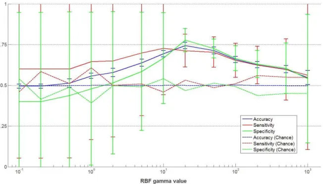
quality was assessed by computing the mean accuracy (blue), the mean sensitivity (red) and the mean specificity (green) over the five cross-validation folds, for different values of the parameter of the RBF kernel function. Vertical bars indicate the standard deviation, and dashed lines correspond to chance level. ... 163
Fig. 79: Speech intention (covert speech) prediction. The patient was first listening to
20
speech was then applied to this covert speech data without any further modification. The blue areas shows the speech intention predicted by this model. ... 164
Fig. 80: Decoding of speech and non-speech states for the second patient. The decoding
quality was assessed by computing the mean accuracy (blue), the mean sensitivity (red) and the mean specificity (green) over the five cross-validation folds, for different values of the σ parameter of the RBF kernel function. Vertical bars indicate the standard deviation, and dashed lines correspond to chance level. ... 165
Fig. 81: Decoding of voicing activity. The decoding quality was assessed by computing
the mean accuracy (blue), the mean sensitivity (red) and the mean specificity (green) over the five cross-validation folds, for different values of the σ parameter of the RBF kernel function. Vertical bars indicate the standard deviation, and dashed lines correspond to chance level. 166
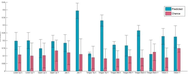
Fig. 82: Best decoding correlation for each articulatory feature. Each bar indicates the
best correlation between predicted and reference articulatory features obtained from the neural-to-articulatory mapping (blue) along with the corresponding best chance level (red). Vertical bars indicate the standard deviations. ... 167
Fig. 83: Optimal delay, context size and number of PCA components for the decoding of each articulatory feature. Top row – Each bar indicates the optimal delay between the
neural and the articulatory features (a negative delay meaning that the neural data occurred before the actual speech). Middle row – Each bar indicates the optimal context size for decoding each articulatory feature. Bottom row – Each bar indicates the optimal delay number of PCA components for decoding each articulatory feature. All rows – the bar plot at the right shows the distribution of the parameters values. ... 168
Fig. 84: Decoding accuracy for each articulatory parameter with respect to the delay between neural and articulatory data. Each plot shows the mean correlation between the
predicted and ground truth values (blue line), as well as chance level (red line), for each articulator and each delay. The delays are in data frames (1 frame = 10ms). A negative delay means that the neural data was considered before the actual speech. Vertical bars correspond to standard deviations. ... 169
Fig. 85: Decoding accuracy for each articulatory parameter with respect to the context size. Each plot shows the mean correlation between the predicted and ground truth
values (blue line), as well as chance level (red line), for each articulator and each context size. The context sizes are in data frames (1 frame = 10ms). Vertical bars correspond to standard deviations. ... 170
Fig. 86: Decoding accuracy for each articulatory parameter with respect to the number of PCA components. Each plot shows the mean correlation between the predicted and
ground truth values (blue line), as well as chance level (red line), for each articulator and each PCA components number. A number of 0 corresponds to not using PCA. Vertical bars correspond to standard deviations. ... 171
Fig. 87: Best decoding correlation for each acoustic feature. Each bar indicates the best
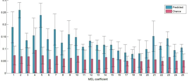
correlation between predicted and reference mel coefficients obtained from the neural-to-articulatory mapping (blue) along with the corresponding best chance level (red). Vertical bars indicate the standard deviations. ... 172
Fig. 88: Optimal delay, context size and number of PCA components for the decoding of each acoustic feature. Top row – Each bar indicates the optimal delay between the neural
21
acoustic feature. Bottom row – Each bar indicates the optimal delay number of PCA components for decoding each acoustic feature. All rows – the bar plot at the right shows the distribution of the parameters values. ... 173
Fig. 89: Decoding accuracy for each acoustic parameter with respect to the delay between neural and acoustic data. Each plot shows the mean correlation between the
predicted and ground truth values (blue line), as well as chance level (red line), for each mel coefficient and each delay. The delays are in data frames (1 frame = 10ms). A negative delay means that the neural data was considered before the actual speech. Vertical bars correspond to standard deviations. ... 174
Fig. 90: Decoding accuracy for each acoustic parameter with respect to the context size. Each plot shows the mean correlation between the predicted and ground truth values (blue
line), as well as chance level (red line), for each mel coefficient and each context size. The context sizes are in data frames (1 frame = 10ms). Vertical bars correspond to standard deviations. ... 175
Fig. 91: Decoding accuracy for each acoustic parameter with respect to the number of PCA components. Each plot shows the mean correlation between the predicted and ground
truth values (blue line), as well as chance level (red line), for each mel coefficient and each PCA components number. A number of 0 corresponds to not using PCA. Vertical bars correspond to standard deviations. ... 176
Fig. 92: Example of predicted and reference acoustic features. Top row – BY2014
acoustic features (black) and the predicted acoustic features using the neural-to-articulatory and the articulatory-to-acoustic mappings (red). Bottom row – Reference patient’s acoustic features (black) and the predicted acoustic features using the neural-to-acoustic mapping (blue). .... 177
Fig. 93: Comparison of the neural-to-acoustic and neural-to-articulatory mapping.
Each bar shows the correlation between predicted and reference mel coefficients fot the neural-to-acoustic (blue) and neural-to-articulatory (red) mappings... 177
Fig. 94: Conceptual view of articulatory-based speech synthesis from neural data.
First, the neural activity is used to detect speech intention in order to enable or disable the speech synthesis (pink path). If speech intention is detected, voicing activity is decoded from the neural data to generate an appropriate excitation signal for voiced and unvoiced sounds (purple path). This neural activity is then decoded into articulatory trajectories which are then converted to mel coefficients using the articulatory-based speech synthesizer (blue path). Finally, the MLSA filter combine the mel coefficients and the excitation signal to synthesize speech (orange path). ... 196
List of tables
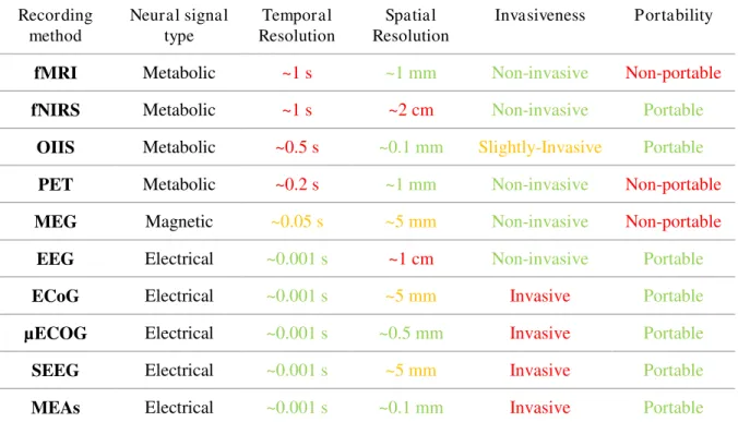
Table 1: Comparison of different neural activity recording methods. Colors are
indicative and reflect the compliance of the method with regard to each criteria for BCI in the context of speech rehabilitation. ... 43
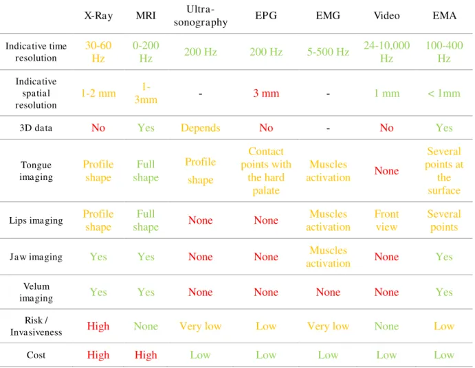
Table 2: Comparison of different articulatory data acquisition methods. Completed
from (Youssef, 2011). Colors are indicative and reflect the compliance of the method with regard to each criteria. ... 57
Acronyms and terms
1D One-Dimensional
2D Two-Dimensional
3D Tree-Dimensional
ANN Artificial Neural Network
ALS Amyotrophic Lateral Sclerosis
ASR Automatic Speech Recognition
BCI Brain-Computer Interface
CG Conjugate Gradient
CNS Central Nervous System
DAE Deep Auto-Encoder
DBN Deep Belief Network
DNN Deep Neural Network
DoF Degrees of Freedom
DTW Dynamic Time Warping
ECoG ElectroCorticoGraphy
EEG ElectroEncephaloGraphy
EGG ElectroGlottoGraph
EMA ElectroMagnetic Articulography
EMG ElectroMyoGraphy
EPG ElectroPalatoGraphy
FMC Face Motor Cortex
fMRI functional Magnetic Resonance Imaging fNIRS function Near-InfraRed Spectroscopy
GD Gradient Descent
GMM Gaussian Mixture Model
GMR Gaussian Mixture Regression
HMM Hidden Markov Model
IPA International Phonetic Alphabet
LFP Local Field Potential
MCD Mel-Cepstral Distortion
MEA Micro-Electrodes Array
MEG MagnetoEncephaloGraphy
MEL Mel-cepstrum
MLE Maximum Likelihood Estimation
MLSA Mel-Log Spectrum Approximation
MMSE Minimum Mean Squared Error
MRI Magnetic Resonance Imaging
MRSE Mean Root Squared Error
MSE Mean Squared Error
PCA Principal Component Analysis
Pdf Probability density function
PET Positron Emission Tomography
rTMS repetitive Transcranial Magnetic Stimulation
SD Standard Deviation
SNR Signal to Noise Ratio
STFT Short Term Fourier Transform
STG Superior Temporal Gyrus
SVM Support Vector Machine
VCV Vowel-Consonant-Vowel sequence
Phonetic notation
All the phonetic transcriptions contained in this thesis manuscript are using the International Phonetic Alphabet (IPA) (Kenyon, 1929).
Introduction
Motivation of research
“Vous n'imaginez pas la gymnastique effectuée machinalement par votre langue pour produire tous les sons du français. Pour l'instant je bute sur le « L », piteux rédacteur en chef qui ne sait plus articuler le nom de son propre journal” (“You cannot imagine the gymnastics automatically performed by your tongue to produce all the French sounds. For now, I stumble on the “L”, pitiful editor who doesn’t know how to articulate the name of his own newspaper.”). This is an extract from the book “Le scaphandre et le papillon”, written by Jean-Dominique Bauby using only the blink of his left eye (about 200.000 for the whole book), while suffering from the locked-in syndrome.
In France, about 300.000 people suffer from a strong speech disorder or aphasia that can often occur after a brain stroke but also in case of severe tetraplegia, locked-in syndrome, neurodegenerative diseases such as Amyotrophic Lateral Sclerosis or Parkinson’s disease, myopathies, or coma. Some of them are not able to communicate at all while they retain cognition and sensation. For these people, speech loss is an additional affliction that worsens their condition: it makes the communication with caregivers very difficult, and more generally, it can lead to profound social isolation and even depression. Therefore, it is crucial for these patients to restore their ability to communicate with the external world.
Current approaches can provide ways to communicate, mostly through a typing process, by analyzing residual eye movements or brain responses to specific stimuli. However, up to several minutes are needed to type a full sentence, while it only requires about three seconds using natural speech, and not all patients can benefits from these systems.
Indeed, speech remains our most natural and efficient way of communicating. But as Jean-Dominique Bauby mentioned, speech is the result of complex muscle movements, controlled by our nervous system. Over the past decades, Brain-Computer Interfaces (BCI) approaches have been increasingly developed to control the motor movements of effectors (e.g., robotic arms or computer screen cursor) with increasing precision, first in animals and more recently in humans. These systems first enabled controlling a small number of degrees of freedom (DoF), typically 1 or 2, while recent studies have reported that subjects were able to simultaneously control up to 10 DoF in complex motor tasks after appropriate training. However, there has been so far no demonstration of the feasibility to restore direct speech using a BCI approach.
The overall objective of this thesis was thus to develop a parametric speech synthesizer that could be used in a BCI paradigm and to design and run clinical trials in order to collect, analyze and decode speech-related brain activity.
There are several difficulties to overcome in order to reach this goal. First, a speech synthesizer suitable for a BCI approach should run in real-time and be robust enough in order to compensate for brain activity decoding errors. Secondly, speech relies on a high number of DoF for which timing is crucial, which are both challenges for BCIs. Third, many brain areas
26
limited, especially when neural recording requires surgery, which makes it hard to collect large data sets.
With the development of machine learning techniques and data acquisition methods for speech-related signals, parametric speech synthesis is now possible using statistical models of huge data sets. Moreover, recent works showed that brain-computer interfaces now allow control of several DoF, up to around 10, with increasing precision, while using neural activity recorded in small brain areas. These advances are first steps toward a brain-computer interface for speech rehabilitation.
Organization of the manuscript
The thesis manuscript is organized as follows.
Part 1 introduces the topics covered by this thesis and their literature, and is divided into
three chapters:
Chapter 1 Introduces brain computer interfaces for communication and the key points to consider when developing such brain-computer interface, including the different cortical areas involved during speech production, the different neural activity recording techniques, as well as the different strategies to decode neural activity.
Chapter 2 is focused on existing approaches for parametric speech synthesis, and more particularly for articulatory-based parametric speech synthesis. It covers as well common ways of acquiring articulatory data.
Part 2 briefly presents the goal of this thesis.
Part 3 describes the articulatory-based speech synthesizer developed during this thesis:
Chapter 3 describes two articulatory-acoustic data sets that were used to perform the speech synthesis. The first corpus was already existing while the second one was specifically recorded from a “reference speaker” for our purpose. Electromagnetic articulography (EMA) was used to acquire articulatory data of the speaker synchronously with the audio speech signal, which was parametrized using mel-cepstrum coefficients.
Chapter 4 focuses on speech synthesis from articulatory data from a “reference speaker” and its evaluation. The mapping from articulatory to acoustic data was performed using a Deep Neural Network (DNN) trained on an articulatory-acoustic dataset. This approach was then evaluated using both objective and perceptive listening tests, and compared to a state-of-the-art approached based on Gaussian Mixture Regression (GMR).
27
new speakers. In a preliminary study, the robustness of the DNN-based articulatory speech synthesizer was assessed using artificially degraded articulatory data as input for the synthesis, and compared to a state-of-the-art GMM model. The articulatory speech synthesizer was adapted to new speakers in order to be controlled in real-time while they were silently articulating.
Part 4 describes preliminary results on analyzing and decoding speech-specific neural
activity:
Chapter 6 presents a way to automatically localize speech-specific brain areas during awake surgery. Such localization is needed in order to optimize the positioning of micro-electrode arrays that can only cover a limited surface of the cortex.
Chapter 7 presents preliminary results on decoding speech features from neural activity. In particular, this chapter is focused on speech intention detection, which consists in predicting, from the neural activity, when a patient intends to speak or not, as well as on voicing activity detection – predicting if the vocal folds are vibrating or not – and the decoding of articulatory trajectories.
Part 5 is an attempt at analyzing the ethical implications of brain-computer interfaces in
general and their development.
Finally, Part 6 summarizes the contributions of this thesis and discusses suggestions for future work.
Part 1: State of the art
Chapter 1: Brain-computer interfaces for speech
rehabilitation
I. Introduction: Brain-computer interfaces for communication
Different solutions for restoring communication in patients with severe paralysis have been developed, most often through a typing process in which letters are selected one by one by exploiting residual physiological signals, such as tracking the eyes direction to control a computer mouse cursor and detecting eye blinks to allow the user to click on the letter pointed by the cursor. However, such solutions are only available for patients with sufficient remaining motor control and only allow to control devices with a small number of degrees of freedom. To overcome this problem, communication systems controlled directly by brain signals have thus started to be developed.
This concept has been pioneered by Farwell and Donchin who proposed a spelling device based on the evoked potential P300 (Farwell and Donchin, 1988), a method that has since been used successfully by a patient with amyotrophic lateral sclerosis (ALS) to communicate (Sellers et al., 2014). The P300 is an event related potential generally elicited when a low-probability expected event occurs during a series of high-probability events and can be recorded using electro-encephalography (EEG). It occurs for instance when a subject actively detects a different sound among a series of identical sounds. Other EEG-based approaches use steady-state potentials tuned at different frequencies (Middendorf et al., 2000). When the retina is exposed to a visual stimulation at a specific frequency (generally from 3 to 75Hz), the brain generates visual evoked potentials at identical frequency called steady state visual potential (SSVP). This natural phenomenum can be exploited by displaying on a screen all the letters blinking at different frequencies so that when the patient focuses on a specific letter, the corresponding SSVP can be detected and the letter identified. These EEG-based approaches present the great advantage of being non-invasive. However, they have been limited by a low spelling speed of a few characters per minute, although recent improvements suggest that higher speed could be achieved (Townsend and Platsko, 2016). Moreover, such tasks are very demanding for the subjects that must remain focused and concentrated during the whole typing process (Käthner et al., 2014; Baykara et al., 2016), thus limiting the use of the device over extensive periods of time.
On the other hand, BCI systems based on intracortical recording, while having the major drawback of being invasive, seem to require less concentration effort from the subject, the external device becoming progressively embodied after a period of training (Hochberg et al., 2006, 2012; Collinger et al., 2013; Wodlinger et al., 2014). Moreover, intracortical recordings allow to capture more information and thus lead to a more precise decoding of the user’s intention. Combining intracortical recording with self-recalibrating algorithms was recently
30
which are then integrated by the soma. The axon is the main conducting unit of the neuron and propagates signals to the other nerve cells.
F ig. 2: Structure of a neuron. A neuron is composed by dendrites, the cell body and an axon that ends by synapses that contact other neurons. The transmission of action potentials at the synapses is generally chemical, by releasing neurotransmitters. Source: thatsbasicscience.blogspot.fr
The cellular membrane of neurons is sprinkled with ion pumps and leaky ion channels. While the membrane is an insulator and a diffusion barrier to the movements of ions – which are electrically charged particles, ion pumps actively push ions across the membrane and establish concentration gradients across the membrane. On the other hand, leaky ion channels passively allow or prevent specific ions from traveling through the cellular membrane down the concentration gradients. The difference in ions concentration gives rise to a difference in electric potential between the interior and the exterior of the cell, the transmembrane potential. At rest, there are concentration gradients of sodium and potassium ions across the cell membrane, with a higher concentration of sodium ions outside the neuron and a higher concentration of potassium ions inside the neuron. These gradients are maintained by sodium/potassium ion pumps which constantly push potassium in and sodium out the cell. The corresponding transmembrane potential is called resting potential. The resting potential is generally close to the potassium reversal potential, arround -70mV, meaning that the intra-cellular medium is more negatively charged than the extra-intra-cellular medium.
A neuron typically receives input signals at the dendrites which are then spread through the soma. The axon of the other nerve cells contact the dendrites at sites called synapses (Fig. 2). The transmission of the neural signal at a synapse is generally chemical, through the release of neurotransmitters. In the case of an excitatory signal, these neurotransmitters open ligand-gated sodium channels, thus allowing sodium to flow into the cell, which increases the transmembrane potential. This flow of sodium ions travels toward the axon hillock, which is the part of the cell body that connects to the axon. Chemically generated synaptic currents are relatively slow phenomena of about 10 to 100 milliseconds. If the sum of all input currents is