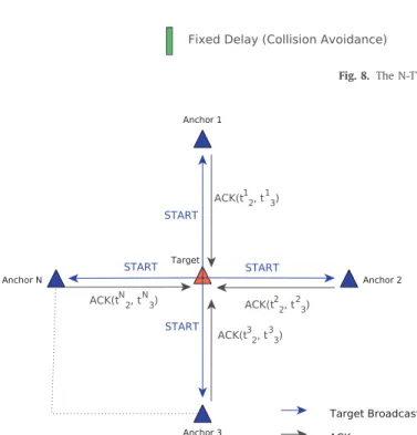
N-TWR: An Accurate Time-of-flight-based N-ary Ranging Protocol for Ultra-Wide Band
20
0
0
Texte intégral
Figure
+7
Documents relatifs