Confidence Estimation for NLP Applications

Publisher’s version / Version de l'éditeur:

ACM Transactions on Speech and Language Processing, 2006

READ THESE TERMS AND CONDITIONS CAREFULLY BEFORE USING THIS WEBSITE.

https://nrc-publications.canada.ca/eng/copyright

Vous avez des questions? Nous pouvons vous aider. Pour communiquer directement avec un auteur, consultez la première page de la revue dans laquelle son article a été publié afin de trouver ses coordonnées. Si vous n’arrivez pas à les repérer, communiquez avec nous à [email protected].

Questions? Contact the NRC Publications Archive team at

[email protected]. If you wish to email the authors directly, please see the first page of the publication for their contact information.

Archives des publications du CNRC

This publication could be one of several versions: author’s original, accepted manuscript or the publisher’s version. / La version de cette publication peut être l’une des suivantes : la version prépublication de l’auteur, la version acceptée du manuscrit ou la version de l’éditeur.

Access and use of this website and the material on it are subject to the Terms and Conditions set forth at

Confidence Estimation for NLP Applications

Gandrabur, S.; Foster, George; Lapalme, G.

https://publications-cnrc.canada.ca/fra/droits

L’accès à ce site Web et l’utilisation de son contenu sont assujettis aux conditions présentées dans le site LISEZ CES CONDITIONS ATTENTIVEMENT AVANT D’UTILISER CE SITE WEB.

NRC Publications Record / Notice d'Archives des publications de CNRC:

Institute for

Information Technology

Institut de technologie de l'information

Confidence Estimation for NLP

Applications *

Gandrabur, S., Foster, G., and Lapalme, G.

2006

* published in the Association for Computing Machinery (ACM) Transactions on Speech and Language Processing (TSLP). 2006. 26 Pages. NRC 48755.

Copyright 2006 by

National Research Council of Canada

Permission is granted to quote short excerpts and to reproduce figures and tables from this report, provided that the source of such material is fully acknowledged.

SIMONA GANDRABUR RALI, Universit´e de Montr´eal and

GEORGE FOSTER

National Research Council, Canada and

GUY LAPALME

RALI, Universit´e de Montr´eal

Confidence measures are a practical solution for improving the usefulness of Natural Language Processing applications. Confidence estimation is a generic machine learning approach for deriving confidence measures. We give an overview of the application of confidence estimation in various fields of Natural Language Processing, and present experimental results for speech recognition, spoken language understanding, and statistical machine translation.

Categories and Subject Descriptors: I.2.7 [Artificial Intelligence]: Natural Language Process-ing—Machine translation; Speech recognition and Spoken language understanding; I.2.6 [Arti-ficial Intelligence]: Learning—Neural Networks; C.4 [Performance of Systems]: —Fault tolerance; Reliability; Modeling techniques; G.3 [Probability and Statistics]: —Statistical computing; Reliability and robustness; F.1.1 [Computation by Abstract Devices]: Models of Computation—Self-modifying machines; J.5 [Computer Applications]: Humanities—Lan-guage translation; Linguistics

General Terms: Algorithms, Design, Experimentation, Reliability, Theory

Additional Key Words and Phrases: confidence measures, confidence estimation, statistical ma-chine learning, computer-aided mama-chine translation, speech recognition, spoken language under-standing

1. CONFIDENCE ESTIMATION FOR NATURAL LANGUAGE PROCESSING AP-PLICATIONS

Despite significant progress in recent years, many NLP technologies are not yet 100% reliable, in the sense that their output is often erroneous. Errors are due to the fact that language itself is typically ambiguous and because of technological lim-itations. Examples are numerous: automatic speech recognition applications (ASR) often return wrong utterances, machine translation (MT) applications frequently produce awkward or incorrect translations, hand writing recognition applications are not flawless, etc.

...

Permission to make digital/hard copy of all or part of this material without fee for personal or classroom use provided that the copies are not made or distributed for profit or commercial advantage, the ACM copyright/server notice, the title of the publication, and its date appear, and notice is given that copying is by permission of the ACM, Inc. To copy otherwise, to republish, to post on servers, or to redistribute to lists requires prior specific permission and/or a fee.

c

We describe experiments in confidence estimation (CE), a generic machine learn-ing approach for estimatlearn-ing the probability of correctness of the outputs of an arbitrary NLP application. In this framework, a baseline application generates a set of one or more output candidates, and a separate confidence estimation com-ponent assigns scores intended to reflect how likely each candidate is to be correct. These scores, called confidence measures, can be used to take appropriate action, such as prompting a user for additional input, when they are judged to be too low. Confidence estimation is related to the technique of reranking, in which the base-line system outputs many alternative answers (for instance, many possible tran-scriptions for a given utterance in speech recognition), which are then re-ordered using more information than was available to the baseline system. The idea is that the baseline system acts as a filter to identify a relatively small set of candidates to be evaluated by a more computationally-expensive reranking system. Rerank-ing has been successfully applied to a number of different NLP problems, includRerank-ing parsing [Collins and Koo 2005], machine translation [Och and Ney 2002; Shen et al. 2004], named entity extractionCollins02 and speech recognition [Collins et al. 2005; Hasegawa-Johnson et al. 2005].

In contrast to reranking, confidence estimation aims only at determining whether a particular output from the baseline system is correct or not. CE typically does not improve the performance of the baseline system; it only attempts to describe it. This task calls for different information than reranking, for instance the degree of noise or uncertainty in input, which is not useful in distinguishing among different possible outputs. In this paper we focus exclusively on CE.

Confidence measures and confidence estimation methods have been used exten-sively in ASR for rejection [Gillick et al. 1997; Hazen et al. 2002; Kemp and Schaaf 1997; Maison and Gopinath 2001; Moreno et al. 2001a]. Instead of focusing on im-proving the output of the baseline system, these methods provide tools for effective error detection and error handling. They have proven extremely useful in making ASR applications usable in practice. Confidence measures have been less frequently used in other areas of NLP, arguably because less practical applications are avail-able in these fields: rejection is useful when an end application can determine the cost of a false output versus an incomplete output and set a rejection threshold accordingly.

In [Gandrabur and Foster 2003] if was first shown how the same methods used in ASR for CE and rejection could be used in machine translation in the context of TransType, an interactive text prediction application where the cost of a wrong output could be estimated both in practice and by a theoretical user model. In [Blatz et al. 2004a] it was noted that CE is a generic approach that could be applied to any technology with underlying accuracy flaws, but results were presented only for machine translation.

Our current paper gives an overview of CE in general and is a first attempt to present CE experiments in practical applications from different NLP fields, SMT and ASR, under a unified framework.

In sections 1–4, we set out a general framework for confidence estimation: section 1 motivates the use of this technique; section 2 defines confidence measures and gives an overview of related work; section 3 describes confidence estimation; and section

4 discusses issues related to evaluation.

In section 5 we present a case study of the use of CE within an ASR application. Section 6 describes how CE can be used for an interactive MT application. We conclude in sections 7 and 8 by enumerating the advantages and the limitations of the use of CE in NLP.

1.1 Why are NLP Technologies difficult?

At a fundamental level, NLP technologies are difficult because the underlying tasks are hard to define precisely. Human judgment about what constitutes a correct answer to a linguistic problem often encompasses many different alternatives, and varies from one person to another. Thus it can be argued that a notion of confidence is intrinsic even to human language processing: sometimes there are only better or worse responses, and it is expedient to be able to quantify this.

More concretely, there are many reasons why NLP performance is still well be-low human levels in most areas. Viewed as a learning problem, language is usually characterized by a sparse data condition, one that is exacerbated by wide variations across domains. Statistical models are overly simplistic, both in order to combat overfitting and because the true statistical structure of language is unknown. Prac-tical problems such as noisy inputs and search errors can lead to further degradation of performance.

1.2 Workarounds to Accuracy Flaws

One response to NLP imperfections is to simply ignore them. Many current NLP-based applications adopt this strategy, which calls for careful management of user expectations. For instance, machine translation output is often billed as being useful for gisting purposes—sufficient to allow a reader to infer the general scope or meaning of the source text, but not to convey precise details.

Another solution, adopted widely in ASR but less so in other fields of NLP, is the use of confidence measures. These are numerical scores assigned to individual outputs that reflect the system’s degree of confidence. Confidence measures allow an application to take remedial action when it judges that an error may have occurred. The canonical example in ASR is to prompt a user to repeat a poorly-recognized utterance. In a machine-translation post-editing application, confidence measures can be used to identify questionable sentence-level translations for human revision. In information retrieval, they can be used to establish a relevance threshold, beyond which documents will not be shown to the user. In general, confidence measures can make NLP applications more natural and more useful.

In many cases, confidence measures can be derived directly from an NLP system. For instance, the probabilistic scores that statistical systems assign to their outputs can fulfill this role. However, the use of a separate confidence estimation component offers more flexibility, because it can easily be recalibrated in response to changes in the operating domain or modifications to the base NLP system. This is the approach to assessing confidence that we emphasize in this paper.

2. CONFIDENCE MEASURES

Consider a generic application that for any given input x ∈ X of a fixed input domain X returns a corresponding output value y ∈ Y of a fixed output domain Y .

Moreover, suppose that this application is based on an imperfect technology, in the sense that the output values y can be correct or false (with respect to some well-defined evaluation procedure). Formally, we can associate a binary tag C ∈ {0, 1}, 0 for false and 1 for correct, to each output y, given its corresponding input x. Practically all NLP applications can be cast in this mold, for example:

—automatic speech recognition (ASR) applications: x is a speech wave and y is the corresponding sequence of words,

—machine translation (MT): x is a sequence of words in a given source language and y is the equivalent sequence of words in a different target language,

—automatic language identification (LI): x corresponds to text and y is the lan-guage the text is written in,

—information retrieval (IR): x is a query for information and y is a document relevant to this query,

—hand writing recognition: x is a hand-written text and y is the equivalent typed text.

A confidence measure is a function c : X × Y × K → I, where: X and Y are input and output domains as described above; K is an abstract domain of additional knowledge sources used to determine the confidence; and I is the confidence range. Typically, I is an interval [a, b] ∈ R such that a lower confidence score is indicative of lower reliability. (Discretizing this interval into specific ranges corresponding to different confidence levels—and ultimately to different actions—is usually left to the end application.)

An important subclass of confidence measures consists of those for which c(x, y, k) is intended to be an estimate of the probability P (C = 1|x, y, k) that y is correct, where C ∈ {0, 1} is a binary correctness judgment for y. Such probabilistic con-fidence measures can be used by the end application to choose the action that minimizes risk in a decision-theoretic setting, provided that the costs associated with different scenarios are known. Indeed, if costs depend dynamically on x and y, risk cannot be minimized without a probabilistic measure.

Alternative probabilistic confidence measures are posterior probabilities P (y|x), which can often be derived directly from statistical NLP systems. However, these are less general than correctness probabilities P (C|x, y) due to the requirement that P

yP (y|x) = 1, which forces the maximum probability of correctness to depend on

the number of correct answers y for a given input x. For problems like machine translation that can have many equally-correct answers, correctness probabilities are preferable because they have a uniform interpretation, independent of x. 3. CONFIDENCE ESTIMATION

CE is a generic machine learning approach for computing confidence measures for a given application. It consists in adding a layer on top of the base application that analyzes the outputs in order to estimate their reliability or confidence. In our work, the CE layer is a model for P (C|x, y, k), the correctness probability for output y, given input x and additional information k.

Such a model could in principle be used to choose a different output from the one chosen by the base system, but it is not typically used this way (otherwise the

confidence layer could be incorporated to improve the base system). Rather, its role is to predict the probability that best answer(s) output by the base application will be correct. To do this, it may rely on information from k that is irrelevant to the problem of choosing a correct output—for example, the length of the source sentence in machine translation, which is often correlated with the quality of the resulting translation.

3.1 Machine-Learning Approaches

The CE model is discriminatively trained over an annotated corpus that consists of (x, y)-pairs, where x is from the application’s input domain and y is the correspond-ing output produced by the application. To avoid overestimatcorrespond-ing performance on new text, this corpus should be disjoint from any material originally used to train the application. Each pair in the corpus is annotated with a label C ∈ {0, 1}; 1 if y is a correct output, 0 otherwise.

The pair (x, y) is represented as a vector of confidence features that captures properties relevant for determining the correctness of the output. Examples of confidence features are:

—the base-model probability estimate (in the case of statistical NLP applications); —input-specific features (e.g. input sentence length, for a MT task);

—output-specific features (e.g. language-model score computed by an independent language model over an output word sequence);

—features based on properties of the search space (e.g. size of a search graph); and —features based on output comparisons (e.g. average distance from the current

output to alternative hypotheses for the same input).

A detailed classification of types of confidence features is given in [Blatz et al. 2004a].

Some of these features—such as the base-model probability—can be used as con-fidence measures in their own right. With a suitable training corpus and machine learning method, we can expect that a CE layer incorporating many features will perform better than any single feature on its own. Various machine-learning meth-ods can be used to combine features, including stacking [Ting and Witten 1997], boosting [Schapire 2001], SVMs [Joachims 1998], neural nets [Bishop 1995], and Maximum Entropy models [Foster 2000; Och and Ney 2002]. In this article we use neural nets to learn combined confidence measures.

3.2 Confidence Estimation with Neural Nets

Our models for confidence estimation are multi-layer perceptrons (MLPs) with a LogSoftMax activation function, trained by gradient descent with a negative-log-likelihood (NLL) criterion. Under these conditions, the outputs of the MLP are guaranteed to be estimates of the conditional correctness probability p(C = 1|x, y, k) [Bishop 1995]. An advantage of MLPs is that the computer resources required for training are modest (unlike SVMs, for example). The ability to train efficiently is important for NLP applications, where the number of training examples may be very large.

We describe experiments with two types of neural nets: MLPs, as described above; and the special case of MLPs that have no hidden layer, which we refer to as single-layer perceptrons (SLPs). This distinction is interesting because MLPs can approximate an arbitrary decision boundary, whereas SLPs are limited to linear decision boundaries. In the following paragraphs we establish a link, first presented in [Gandrabur and Foster 2003], between SLPs and Maximum Entropy models.

For the problem of estimating p(y|x) for a set of classes y over a space of input vectors x, a single-layer neural net with softmax outputs takes the form:

p(y|x) = exp(~αy· x + b)/Z(x)

where ~αyis a vector of weights for class y, b is a bias term, and Z(x) is a

normaliza-tion factor, the sum over all classes of the numerator. A maximum entropy model is a generalization of this in which an arbitrary feature function fy(x) is used to

transform the input space as a function of y:

p(y|x) = exp(~α · fy(x))/Z(x).

Both models are trained using maximum likelihood methods. Given M classes, the maximum entropy model can simulate a SLP by dividing its weight vector into M blocks, each the size of x, then using fy(x) to pick out the yth block:

f_{y(x) = (01, . . . , 0y−1, x, 0y+1, . . . , 0M, 1),} where each 0i is a vector of 0’s and the final 1 yields a bias term.

The advantage of maximum-entropy models is that their features can depend on the target class. For natural-language applications where target classes correspond to words, this produces an economical and powerful representation. However, for CE, where the output is binary (correct or incorrect), this capacity is less interest-ing. In fact, there is no a priori reason to use a different set of features for correct outputs or incorrect ones, so the natural form of a maxent model for this problem is identical to a SLP (modulo a bias term). Therefore our experiments can be seen as comparisons between maxent models and neural nets with a hidden layer. 3.3 Related Work

The most extensive application of CE in NLP is within the field of ASR, where confidence measures are typically used to determine whether or not to ask a user to repeat an utterance, as described below in section 5. In ASR, approaches based on a separate CE layer tend to predominate, although there is also work on posterior probability confidence measures derived from nbest lists or word lattices [Mangu et al. 2000; Wessel et al. 2001]. Many different machine-learning algorithms have been used for training CE layers, including Adaboost [Carpenter et al. 2001], naive Bayes [Sanchis et al. 2003], Bayesian nets [Moreno et al. 2001b], neural networks [Guillevic et al. 2002; Kemp and Schaaf 1997; Weintraub et al. 1997; Zhang and Rudnicky 2001a], boosting [Moreno et al. 2001b], support vector machines [Ma et al. 2001; Zhang and Rudnicky 2001a], linear models [Gillick et al. 1997; Kemp and Schaaf 1997; Moreno et al. 2001b], and decision trees [Kemp and Schaaf 1997; Moreno et al. 2001b; Neti et al. 1997; Zhang and Rudnicky 2001a]. Roughly half of this work concerns CE for probabilistic confidence measures, and half concerns non-probabilistic measures (ie, scores derived from binary classifiers). The standard

methods for evaluating CE performance, discussed in the next section, have also emerged from work in ASR, eg [Siu and Gish 1999] and [Maison and Gopinath 2001].

There is a more recent, but growing, body of work on CE for machine translation and related fields. In [Gandrabur and Foster 2003], a neural-net CE layer is used to improve estimates of correctness probabilities for text predictions in a machine-assisted translation tool. Blatz et el [Blatz et al. 2004b] report on an extensive study to investigate word- and sentence-level CE on MT output, using Naive Bayes and neural net classifiers; a major conclusion is that noise in automatic MT evaluation metrics makes it difficult to determine correctness at the sentence level. Quirk [Quirk 2004] suggests the use of human assessments to get around this problem, and finds that training on a small set of human annotated data leads to better performance, when evaluated on similar data, than does training on a much larger automatically annotated corpus. Finally, Ueffing [Ueffing and Ney 2005] improves on the word-level CE techniques of [Blatz et al. 2004b] by using a general phrase-based translation model, independent from the base MT system, and by optimizing log-linear parameters in the CE layer to improve confidence error rate directly.

CE has also been used in other areas of NLP. [Manmatha and Sever 2002] describe a form of confidence estimation for combining the results of different query engines in information retrieval. [Delany et al. 2005] describe an ad hoc ensemble-based approach to combining confidence features in a spam-filtering application. [Xu et al. 2002] use a mixture of empirical correctness probabilities for single features (such as answer type) to select a response from either a web-based or a traditional question answering system. [Culotta and McCallum 2004] study the problem of confidence estimation in an information extraction system based on linear-chain conditional random fields. They find that posterior probabilities derived using the forward-backward algorithm from the base system’s model outperform related ad hoc methods, and give about the same performance as an external maximum-entropy CE layer that uses the posterior estimates as features. Another important use of CE is in active learning, where correctness probabilities can be used to select informative examples for human annotation [Culotta and McCallum 2005]. Finally, CE has applications outside of NLP, for instance in CPU branch prediction for instruction-level parallelism [Grunwald et al. 1998].

4. EVALUATION

In this section we discuss two aspects of evaluation that are pertinent to CE: (1) evaluation of correctness of the base application outputs, and (2) evaluation of the accuracy and usefulness of confidence measures.

4.1 Evaluation of Correctness

As described above, the approach to CE that we promote in this paper requires examples of system input and output labelled with binary correctness judgments. These are used for both training and evaluation purposes.

Producing such data requires extensive human effort and is subject to typical problems such as noisy input and inter-annotator disagreement. Nevertheless, it is relatively straightforward for problems such as speech recognition and text clas-sification for which there is at least nominally one right answer. In such cases,

standard data sets labelled with the correct answer can be established, and the cor-rectness status for a given system’s output over these data sets can be determined automatically.

The situation is more complicated for problems like machine translation and au-tomatic summarization for which the answers are multiple and less clearly defined. Here the best approach would be to have humans evaluate all system outputs, but this is often too expensive, as it needs to be done separately for different systems and even for different versions of the same system. An alternative is to establish standard data sets containing a set of correct answers for each input, from which the status of a system output can be calculated using some distance measure such as the well-known BLEU metric in machine translation [Papineni et al. 2001]. Binary correctness judgments can then be derived by thresholding this distance measure. 4.2 Evaluation of Confidence Measures

Since the motivation for using confidence measures is to improve an application, the ultimate gauge of their success is the gain in end-to-end performance. However, it is also useful to have metrics that allow for more direct evaluation of confidence measures. We use two such metrics:

—Receiver Operating Characteristic (ROC) curves, and related quantitative metrics for assessing discriminability [Zou 2004]; and

—Normalized Cross Entropy (NCE) for measuring the relative decrease in uncer-tainty about the correctness of the application outputs produced by the confi-dence measure [NIST 2001].

ROC curves apply to any confidence score (probabilistic or not), and are valuable for comparing discriminability and determining optimal rejection thresholds for specific application settings. NCE applies only to probabilistic measures, and tests the accuracy of their probability estimates; it is possible for such measures to have good discriminability and poor probability estimates, but not the converse. In the following sections, we briefly describe each metric.

4.2.1 ROC curves. Any confidence measure c(x, y, k) can be turned into a bi-nary classifier by choosing a threshold θ and judging the system output y to be correct whenever c(x, y, k) ≥ θ. Over a given dataset consisting of pairs (x, y) la-belled for correctness as defined in section 3.1, the performance of the classifier can be measured using standard statistics like accuracy. The statistics used for ROC are correct acceptance (CA) and correct rejection (CR): the proportion of pairs scor-ing above θ that are in fact correct, and the proportion scorscor-ing below θ that are incorrect.

In general, different values of θ will be optimal for different applications. An ROC curve summarizes the global performance of c(x, y, k) by plotting CR(θ) versus CA(θ) as θ varies. An advantage of using CA and CR for this purpose is they range from 0 to 1 and 1 to 0, respectively, as θ ranges from the smallest value of c(x, y, k) in the dataset to the largest. This means that ROC curves always connect the points (1,0) and (0,1) and thus are easy to compare visually (in contrast to other plots such as recall versus precision). Better curves are those that run closer to the top right corner, and the best possible connects (1,0), (1,1), and (0,1) with

straight lines. This corresponds to perfect discriminability, with all correct points (x, y) assigned higher scores than incorrect points. Curves “below” the diagonal are equivalent to those above, with the sign of c(x, y, k) reversed.

A quantitative metric related to ROC curves is IROC, the integral below the curve, which ranges from 0.5 for random performance to 1.0 for perfect perfor-mance. This metric is similar to the Wilcoxon rank sum statistic [Blatz et al. 2004a]. Alternatively, one can choose a fixed operating point for CA (for instance 0.80), and compare the corresponding CR values given by difference confidence measures.

4.2.2 Normalized Cross Entropy. NIST introduced the Normalized Cross En-tropy (NCE) measure as the cross enEn-tropy (mutual information in this context) between the correctness of the system’s output y and its probabilistic confidence score, normalized by a baseline cross entropy:

 Hbase+ X correct y log2P (C = 1|x, y) + X incorrect y log2P (C = 0|x, y)  /Hbase

where Hbase = n log2pc+ (N − n) log2(1 − pc), pc is the prior probability of

cor-rectness, and n is the number of correct outputs out of N total outputs.

The idea of NCE is to allow for comparison of confidence measures across different test sets by correcting for the effect of prior probabilities, which tend to boost raw cross-entropy scores when they are high. The term Hbase is proportional to the

maximum cross entropy obtainable by assigning a fixed probability of correctness to all examples when the prior is pc. NCE scores normally range from 0 when

performance is at this baseline to 1 for perfect probability estimates, although negative scores are also possible.

5. CONFIDENCE ESTIMATION FOR AUTOMATIC SPEECH RECOGNITION This section describes the use of CE within an ASR application, first presented in [Guillevic et al. 2002], where a human user interacts by speaking with a system, in our case a directory assistant application.

The user says an utterance, either a phrase or a short command, and the ASR application interprets the utterance into a sequence of words, called recognition hy-pothesis. Then, a Spoken Language Understanding (SLU) module extracts meaning from the recognition hypothesis by interpreting it into a sequence of concepts or semantic slots.

The example below illustrates the interaction between a human user and an ASR directory application. A user wanting to reach a certain “McPhearson” on the telephone, utters the desired name when prompted by the application. The ASR engine returns three alternative recognition hypotheses as a N-best set:

1 McPhearson 2 Paul McPhearson 3 Mike Larson

A robust parser transforms each recognition hypothesis into one or more semantic hypotheses or semantic interpretations, that is, a sequence of concepts:

1 (userID=103, LastName=McPhearson) 2 (userID=103, FullName=Paul McPhearson) 2 (userID=103, LastName=McPhearson) 3 (userID=217, FullName=Mike Larson) 3 (userID=217, LastName=Larson) 3 (userID=315, LastName=Larson)

A concept is a key-value pair; in our example, the keys are userID, LastName and FullName. For instance, the second recognition hypothesis “Paul McPhear-son” has two different semantic interpretations: both corresponding to the same destination (userID=103), one corresponding to a full parse (FullName=Paul McP-hearson) and the other only a partial parse that leaves out the first name “Paul” (LastName=McPhearson).

A dialog manager then decides that the confidence level of the destination concept userID_{=103 is sufficiently high to transfer the call this destination.}

This application relies on concept-level confidence scores for designing its dialog strategies. For instance, if the confidence level of a destination is too low, the application might decide to prompt the user for a confirmation, such as “Would you like to talk to Paul McPhearson?”. Alternatively, if all confidence levels of semantic interpretations are too low, the application might decide to reject the entire utterance and prompt for a repetition, such as: “Sorry, I did not understand. Could you please repeat your request?”.

Typical confidence measures for ASR applications first determine the reliability of the ASR results at the word level and then at the utterance level [Wessel et al. 2001; Stolcke et al. 1997; Sanchis et al. 2003; Carpenter et al. 2001; Hazen et al. 2000; Moreno et al. 2001b; Zhang and Rudnicky 2001b]. However, in speech un-derstanding systems, recognition confidence must be reflected at the semantic level in order to be able to apply various confirmation strategies directly at the concept level. In the previous example, the application is not concerned about how well the word “Paul” was recognized when deciding to transfer the call to Paul McPhearson. It only needs to take into account how confident the destination userID=103 is.

Concept-level confidence scores can be obtained by computing word and utter-ance confidence scores and feeding them to the natural language processing unit in order to influence its parsing strategy [Hazen et al. 2000]. This approach is mostly justified when semantic interpretation tends to be a time-consuming pro-cessing task: the time to complete a robust parsing over a large N-best list (or equivalent word-lattice) is reduced by only focusing on areas of the word-lattice where recognition confidence is high.

Alternatively, a confidence score can be computed directly at the concept level [San-Secundo et al. 2001]. This method has the advantage of being more complete: it enables taking parsing-specific and semantic consensus information into account when computing the concept-level confidence score.

In the following experiments we first compute a confidence score at the word level, based mainly on acoustic features computed over N-best lists (or the equivalent word-lattices). Secondly, we parse the utterances and use the word-level confidence score (among other features) to compute a concept-level confidence score.

Confidence scores are computed using the CE approach: we train MLPs to esti-mate the probability of correctness of recognition results on two levels of granularity:

word-level and concept-level. The training is supervised, based on an annotated corpus consisting of various utterances and their corresponding recognition and se-mantic hypotheses, annotated as correct or wrong at at word-level, respectively concept-level.

We use the same corpus for both CE tasks, consisting of 40,000 utterances. We split our corpus into three sets: 49/64 of the data for training, 7/64 for validation and the remaining 8/64 for testing.

5.1 Word-Level CE for ASR

For each utterance in the corpus, we generate ASR results as sets of N-best recog-nition hypotheses with N=5.

A per-word timing information is available, that indicates the precise start and end frame of the speech signal (the minimal unit the signal is divided into) that each word corresponds to. This timing information allows us to recover the word-lattice structure from the N-best lists.

Each word in a recognition hypothesis constitutes a training/testing example for the word-level CE task: a number confidence features and a correct/wrong tag are computed for each word.

A word is tagged as correct if it can be found in roughly the same position in the utterance’s reference transcription and incorrect otherwise. This step is performed by aligning the hypothesis and the reference word sequences using a dynamic pro-gramming algorithm with equal cost for insertions, deletions, and substitutions. As a result, each hypothesized word is tagged as either: insertion, substitution, or ok, with the ok words tagged as correct, while the others are tagged as incorrect. Note that the comparison between two words is based on pronunciation, not orthography.

We use four different word-level confidence features:

Frame-weighted raw score. This corresponds to the log-likelihood that the recog-nized word is correct given the speech signal that it was aligned to, as estimated by the probabilistic acoustic models used within the ASR application. This score is computed by averaging the acoustic score (the log-likelihood estimated by the acoustic models used in the ASR system that the recognized word-segment is correct given the speech signal) over all frames in a word.

Frame-weighted acoustic score. This is the frame-weighted raw score normalized by an on-line garbage model [Caminero et al. 1996]. It is the base word score originally used by the underlying ASR application;

State-weighted acoustic score. This score is similar with the frame weighted acous-tic score. The difference is that the score is averaged not over frames but over Hidden Markov Model (HMM) states corresponding to the word;

Word length. The number of frames of each word.

Given the four word-level features mentioned above, plus the correct tag, we train a MLP network with two nodes in the hidden layer and a LogSoftMax activation function, using gradient descent with a negative-log-likelihood (NLL) criterion. In choosing the MLP architecture (the number of hidden units and layers) we are making a trade-off between: classification accuracy and robustness: more complex architectures (with more hidden units and/or and additional layer) seemed to over

Score NCE CR Frame-weighted acoustic score 0.25 34% CE word score 0.32 47%

Table I. Correct Rejection (CR) rate for an acoustic word score classifier using a MLP network with two nodes in the hidden layer with a correct acceptation rate of 95%

fit the data, even when early training stopping was performed, and were more sensitive to small changes in the training corpus. The MLP was trained to estimate the probability of a word being correct, according to its confidence features. Prior to being fed to the network, the features are scaled by removing the mean and projecting the feature vectors on the eigenvectors computed on the pooled-within-class covariance matrix. The pooled matrix is the one used in Fisher’s Linear Discriminant Analysis.

As shown in table I, at a correct acceptance (CA) rate of 95%, we are able to boost our correct rejection (CR) rate from 34% to 47%. This represents a 38% relative increase in our ability to reject incorrect words. We also measured the relative performance of our new word score using the Normalized Cross Entropy (NCE) introduced by NIST. We are able to boost the entropy from 0.25 to 0.32.

This means that the new word-level confidence score is more discriminative than the original per-word acoustic score provided by the ASR engine. This improvement leads to better discriminability at the concept level, as will be described in the following section.

5.2 Concept-Level CE for SLU

Using the same experimental set-up as in the preceding section on word-level CE for ASR, we applied the CE approach for SLU, namely at the concept (semantic slot) level.

The start and end times of a semantic slot are respectively defined as the start time of the first word and the end time of the last word that make up the slot. This timing information allows us to obtain a concept-level lattice corresponding to each recognition hypothesis N-best list produced by the ASR engine.

Prior to describing the concept-level confidence features, we define the notion of normalized hypothesis a posteriori probabilities used in the definition of our confi-dence features.

5.2.1 Normalized Hypothesis A Posteriori Probabilities. The recognition hy-potheses (sometimes also referred to as sentences) within an N-best set are ordered according to their sentence score, that is the log-likelihood of the joint probability of the acoustic scores and the language model probabilities of the word sequence: the higher the sentence score, the higher the estimated probability of correctness of the hypothesis and the higher its rank within the N-best set.

The sentence score is very appropriate for ranking hypotheses, but does not not give an indicative absolute confidence measure because it is greatly affected by the sentence length: it is a point probability computed by multiplying the individual word acoustic and language scores. Therefore, longer sentences do not necessarily mean lower probability of correctness. We define the normalized hypothesis score as the posterior probability to obtain a measure that is more robust to sentence

rank sentence Si ∆i k∆i pi pˆi 1 McPhearson −5610.114 0.0 0.0 1.0 0.9033 2 Paul McPhearson −5647.917 −37.803 −2.835 0.0587 0.0530 3 Mike Larson −5650.505 −40.391 −3.029 0.0483 0.0436 Table II. Computation of a posteriori hypothesis probabilities on three recognition hypotheses and the corresponding sentence scores

length.

Given a set of N-best recognition hypotheses Hi with their corresponding

sen-tence scores Si, we compute the normalized hypothesis a posteriori probabilities ˆpi

according to the following formula:

pi= exp [k∆i] , and pˆi = pi/ N

X

j=0

pj.

where the constant k has been set experimentally to 0.075 in our applications, and ∆i= Si− S0:

In table II we illustrate the computation of a posteriori hypothesis probabilities ˆ

pion an example of three recognition hypotheses and their corresponding sentence

scores Si.

In the following sections, we will first describe our concept-level confidence fea-tures, then the labeling method for these concepts and finally our experimental results.

5.2.2 Confidence Features. For each semantic slot, we consider six confidence features:

—word confidence score average;

—word confidence score standard deviation; —semantic consensus;

—time consistency;

—fraction of unparsed words per hypothesis; —fraction of unparsed frames per hypothesis.

The last two confidence features are computed for an entire semantic hypothesis. Semantic consensus and time consistency are similar to slot a posteriori probabil-ities. Mangu [Mangu et al. 2000; Wessel et al. 2001] uses a similar scheme to compute word posteriors and consensus-based confidence features.

Word Confidence Score Average and Standard Deviation are computed over all words in a slot.

Semantic Consensus is a measure of how well a semantic slot is represented in the N-best ASR hypotheses. For each semantic slot value, we sum the normalized hypothesis a posteriori probabilities of all hypotheses containing that slot. The measure does not take into account the position of the slot within the hypothesis.

Time Consistency is related to the semantic consensus described above. For a given slot, we add the normalized a posteriori probabilities of all hypotheses where the slot is present and where the start / end times match. The start and

CR

Features NCE CA = 90% CA=95% CA=99% base-line: AC-av 0.32 59% 36% 6% CE-av, CE-sd 0.35 64% 46% 15%

SC 0.48 81% 66% 21%

AC-av, CE-av/sd, SC, TC 0.55 86% 70% 21%

all 0.56 87% 71% 27%

Table III. CA/CR rates obtained with semantic slot classifiers trained on various subsets of confidence features: the first column gives the features used in each case with the following abbreviations: AC-av=word acoustic score average, av=word confidence score average, CE-sd=word confidence score standard deviation, SC= semantic consensus, TC=time consistency FUW=fraction of unparsed words, FUF=fraction of unparsed frames. The second column gives the normalized cross-entropy (NCE). The last three columns give the correct rejection rates at a given correct acceptance rate (CA)

end frames for each hypothesized word are given by the ASR and then translated into a normalized time scale. The start and end times of a semantic slot are then respectively defined as the start time of the first word and the end time of the last word that make up the slot.

Fraction of unparsed words and frames indicates how many of the hypothesized words are left unused when generating a given slot value. The classifier will learn that a full parse is often correlated with a correct interpretation, and a partial parse with a false interpretation. The measure of unparsed frames is similar to the measure of unparsed words, with the difference that the words are weighted by their length in number of frames.

5.2.3 Tag - Classifier. We tag each semantic slot as either “correct” or “incor-rect”. A semantic slot is “correct” if it appears in the list of slots associated with the reference, regardless of its position.

We feed the six measures mentioned above into an MLP with five hidden neurons. The features are pre-processed before being fed to the network by removing the mean and projecting the feature vector on the eigenvectors of the pooled-within-class covariance matrix.

5.2.4 Results. We train different MLPs using various subsets of features. We measure the performance of the resulting semantic slot classifiers by analyzing the correct rejection (CR) ability at various correct acceptance (CA) rates given in table III.

We see that, by feeding our six measures into a MLP, we enhance the performance of a baseline that uses only the average of the original frame-weighted acoustic word scores. The entropy jumps from 0.32 to 0.56 and the CR rate goes from 36% to 71% for a CA rate of 95%.

In the computation of the semantic consensus and time consistency measures, the occurrence rates of slots in the N-best set are weighted by the normalized hypothesis a posteriori probabilities. In order to measure the impact of these weights, we build classifiers based on these features computed with and without the weights, assuming equal probabilities for all hypotheses. Results are presented in table IV and show an important impact of the weights on the discriminability of the classifiers.

CR Features NCE CA = 90% SC, TC without hypAPostProb 0.39 68% SC, TC with hypAPostProb 0.48 81%

Table IV. Impact of normalized a posteriori hypothesis weights (hypAPostProb) on CA/CR rates. SC = semantic consensus, TC = time consistency.

usefulness of an ASR application. The CE layer produces a combined confidence score that estimates the probability of correctness of an output. This score could be used to discriminate effectively between correct and wrong outputs. We now show how the same approach can be applied to a Machine Translation task. 6. CONFIDENCE ESTIMATION FOR MACHINE TRANSLATION

Confidence measures have been introduced in Statistical Machine Translation (SMT) [Gandrabur and Foster 2003] in the context of TransType, an interactive text pre-diction application, then by [Ueffing et al. 2003]. CE for SMT was the subject of a JHU CLSP summer workshop in 2003 [Blatz et al. 2004a; 2004b].

The application we are concerned with is an interactive text prediction tool for translators, called TransType [Foster et al. 1997; Langlais et al. 2004]. The system observes a translator as he or she types a text and periodically proposes extensions to it, which the translator may accept as is, modify, or ignore simply by continuing to type. With each new keystroke the translator enters, TransType recalculates its predictions and attemps to propose e new completion to the current target text segment. Figure 11 _{shows a TransType screen during a translating session.}

There are several ways in which such a system can be expected to help a trans-lator:

—when the translator has a particular text in mind, the system’s proposals can speed up the process of typing it

—when the translator is searching for an adequate formulation, the proposals can serve as suggestions

—when the translator makes a mistake, the system can provide a warning, either implicitly by failing to complete the mistake or explicitly by attaching an anno-tation for later review

The novelty of this project lies in the mode of interaction between the user and the machine translation (MT) technology on which the system is based. In previous attempts at interactive MT, the user has had to help the system analyze the source text in order to improve the quality of the resulting machine translation. While this is useful in some situations (for example, when the user has little knowledge of the target language), it has not been widely accepted by translators, in part because it requires capabilities (in formal linguistics) that are not necessarily those of a translator. Using the target text as the medium of interaction results in a tool that is more natural and useful for translators.

1_{More information about the project and an interactive demonstration is available at http://} rali.iro.umontreal.ca/Traduction/TransType.en.html

Fig. 1. Screen shot of a TransType prototype. Source text is on the left half of the screen, whereas target text is typed on the right. The current proposal appears in the target text at the cursor position.

This idea poses a number of technical challenges. First, unlike standard MT, the system must take into account not only the source text but that part of the target text which the user has already keyed in. This section will mainly explore how the tool can limit its proposals to those in which it has reasonable confidence but we have also explored how it should adapt its behavior to the current context, based on what it has learned from the translator [Nepveu et al. 2004].

If the system’s suggestions are right, then reading them and accepting them should be faster than performing the translation manually. However, if prediction suggestions are wrong, the user loses valuable time reading through wrong predic-tions before discarding them. Therefore, the system must ideally find an optimal balance between presenting the user with predictions or “acknowledging its igno-rance” and not proposing unreliable predictions. Further complications arise from the fact that longer predictions are typically less reliable and take longer to read, though they save more time if accepted. For this reason, we adopted a flexible prediction length. Suggestions may range in length from 0 characters to the end of

the target sentence; it is up to the system to decide how much text to predict in a given context, balancing the greater potential benefit of longer predictions against a greater likelihood of being wrong, and a higher cost to the user (in terms of distraction and editing) if they are wrong or only partially right.

An avant-garde tool like this one has to be tested and its impact evaluated in au-thentic working conditions, with human translators attempting to use it on realistic translation tasks. We have conducted user evaluations and collected for assessing the strengths and weaknesses both of the system and the evaluation process itself. Part of this data was used for comparing different combinations of parameters in the following experimentations.

In the project’s final evaluation rounds, most of the translators participating in the trials registered impressive productivity gains, increasing their productivity from 30 to 55% thanks to the completions provided by the system. The trials also served to highlight certain modifications that would have to be implemented if the TransType prototype is to be made into a translator’s every day tool: e.g. the ability of the system to learn form the users’ corrections, in order to modify its underlying translation models.

6.1 CE for TransType

Our CE approach for TransType consists in training neural nets to estimate the conditional probability of correctness

p(C = 1| ˆw_{m, h, s, {wm}1_{, . . . , wm}n_})

where ˆw_{m= wm}1 _{is the most probable prediction of length m from a N-best set of} alternative predictions according to the base model.

In our experiments the prediction length m varies between 1 and 4 and n is at most 5. As the N-best predictions {w1

m, . . . , w n

m} are themselves a function

of the context, we will note the conditional probability of correctness by p(C = 1| ˆw_{m, h, s).}

The data used in our experiments originates from a Hansard English-French bi-text corpus. In order to generate the train and test sets, we use 1.3 million (900 000 for training and 400 000 for testing purposes) translation predictions for each fixed prediction length of one, two, three and four words, summing to a total of 5.2 million prediction examples characterized by their confidence feature vector.

Each translation prediction of the test and training corpus is automatically tagged as correct or incorrect. A translation prediction wm is tagged as correct if an

identical word sequence is found in the reference translation, properly aligned. This is a very crude and severe tagging method. It could be relaxed by using multiple reference translations and more sophisticated ways of determining whether two translations are equivalent, rather than requiring identity.

For each original translation model, we experimented with two different CE model architectures: MLPs with one hidden layer containing 20 hidden units and one with 0 hidden units, also referred to as single layer perceptron (SLP).

Moreover, for each native model, CE model architecture pair, we train five sep-arate CE models: one for each fixed prediction length of one, two, three or four words, and an additional model for variable prediction lengths of up to four words. Training and testing of the neural nets was done using the open-source

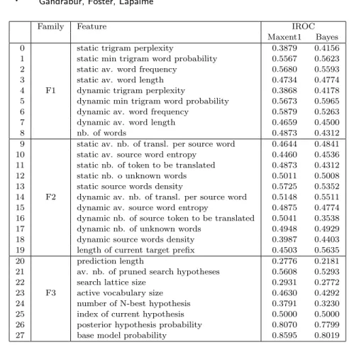
machine-Family Feature IROC Maxent1 Bayes 0 static trigram perplexity 0.3879 0.4156 1 static min trigram word probability 0.5567 0.5623 2 static av. word frequency 0.5680 0.5593 3 static av. word length 0.4734 0.4774 4 F1 dynamic trigram perplexity 0.3868 0.4178 5 dynamic min trigram word probability 0.5673 0.5965 6 dynamic av. word frequency 0.5879 0.5263 7 dynamic av. word length 0.4659 0.4500 8 nb. of words 0.4873 0.4312 9 static av. nb. of transl. per source word 0.4644 0.4841 10 static av. source word entropy 0.4460 0.4536 11 static nb. of token to be translated 0.4873 0.4312 12 static nb. o unknown words 0.5011 0.5008 13 static source words density 0.5725 0.5352 14 F2 dynamic av. nb. of transl. per source word 0.5148 0.5511 15 dynamic av. source word entropy 0.4875 0.4774 16 dynamic nb. of source token to be translated 0.5041 0.3538 17 dynamic nb. of unknown words 0.4948 0.4929 18 dynamic source words density 0.3987 0.4403 19 length of current target prefix 0.4503 0.5635 20 prediction length 0.2776 0.2181 21 av. nb. of pruned search hypotheses 0.5608 0.5293 22 search lattice size 0.2931 0.2772 23 F3 active vocabulary size 0.4630 0.4292 24 number of N-best hypothesis 0.3791 0.3230 25 index of current hypothesis 0.5000 0.5000 26 posterior hypothesis probability 0.8070 0.7799 27 base model probability 0.8595 0.8019 Table V. Confidence features. Description and discriminability for predictions of m = 1, ..., 4 words. The second column describes the families of features : F1 features capture the intrinsic difficulty of the source sentence; F2 features reflect how hard s is to translate; F3 features reflect how hard s is for the current model to translate. The last two columns are the IROC values obtained with each feature.

learning library Torch [Collobert et al. 2002].

6.1.1 Confidence Features. The features can be divided into three families (Ta-ble V):

—F1 capture the intrinsic difficulty of the source sentence s; —F2 reflect how hard s is to translate in general;

—F3 reflect how hard s is for the current model to translate.

For the first two families, we used two sets of values: static ones that depend on s and dynamic ones that depend on only those words in s that are still untranslated, as determined by an IBM2 word alignment between s and h. The features are listed in table V. The average number of translations per source word were computed according to an independent IBM1 model (features 9,14). Features 13 and 18 are the density of linked source words within the aligned region of the source sentence.

6.2 Experimental Results

We performed experiments to test the discriminability of scores (sections 6.2.1 – 6.2.3). To compare the discrimination capacity of scoring functions, we use ROC curves and the integral of the ROC curve, or IROC introduced in section 4.2.1. We also compare scoring functions by fixing an operational point at CA = 0.80 and observing the corresponding CR values.

To establish usability improvements in terms of timing speed due to the use of the CE layer we use a user-model simulation [Foster et al. 2002] (section 6.2.4). For a prediction of a given length, this model gives the time benefit to the user if the prediction is correct, as well as the cost if it is not. It was developed by analyzing data collected in an original human trial with TransType. By combining the estimates of correctness from the CE layer with predicted costs from the user model, we can choose the optimum length of prediction to make in any given context.

Finally, we will test the usefulness of the CE layer in a different setting: for combining translation prediction outputs from separate independent translation models through a simple maximum confidence score voting scheme (section 6.2.5). 6.2.1 Discriminability: CE versus and Native SMT Probabilities. In our setting, the tokens are the ˆw_{mtranslation predictions and the base-model score function is} the conditional probability p(C = 1| ˆw_{m, h, s).}

The first question we wish to address is whether we can improve the correct/false discrimination capacity by using the probability of correctness estimated by the CE model instead of the native probabilities.

For each SMT model we compare the ROC plots, IROC and CA/CR values obtained by the native probability and the estimated probability of correctness output by the corresponding SLPs (also noted as mlp-0-hu) and the 20 hidden units MLPs on the one-to-four words prediction task.

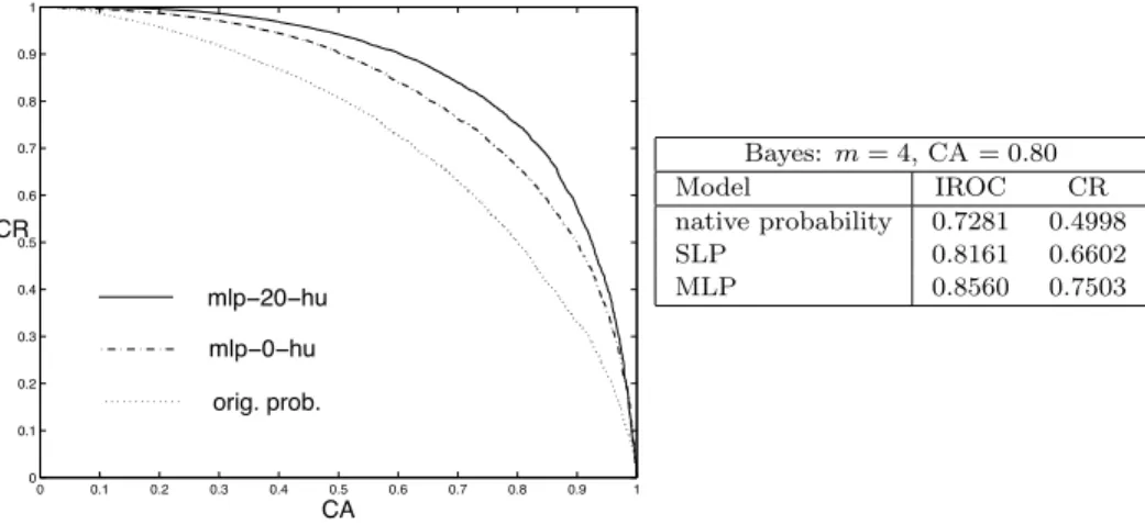
Results obtained for various length predictions of up to four words using the Bayes models are summarized in table VI. At a fixed CA of 0.80 we obtain the CR increases from 0.6604 for the native probability to 0.7211 for the SLP and 0.7728 for the MLP. The overall gain can be measured by the relative improvements in IROC obtained by the SLP and MLP models over the native probability, that are respectively 17.06% and 33.31%.

The improvements obtained in the fixed-length four-words-prediction tasks with the Bayes model, shown in table VII, are even more important: the relative im-provements on IROC are 32.36% for the SLP and 50.07% for MLP.

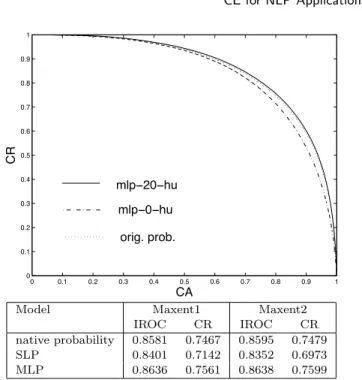
However, the results obtained in the Maxent models are not so good, arguably because the Maxent models are already discriminantly trained. The the SLP CR actually drops slightly, indicating that linear separation was too simplistic and that additional features only added noise to the already discriminant Maxent score. The MLP CR increases slightly to a 4.80% relative improvement in the CR rate for the Maxent1 model and only 3.9% for the Maxent2 model (Table VIII). The results obtained with the two Maxent models being similar, we only give the ROC curve for the Maxent2 model.

It is interesting to note that the native model prediction accuracy did not affect the discrimination capacity of the corresponding probability of correctness of the

0 0.1 0.2 0.3 0.4 0.5 0.6 0.7 0.8 0.9 1 0 0.1 0.2 0.3 0.4 0.5 0.6 0.7 0.8 0.9 1 CA CR mlp−20−hu mlp−0−hu orig. prob. Bayes: m = 1, . . . , 4, CA = 0.80 Model IROC CR native probability 0.8019 0.6604 SLP 0.8357 0.7211 MLP 0.8679 0.7728

Table VI. Bayes model, number of words m = 1, . . . , 4 :ROC Curve and comparison of discrimi-nation capacity between the Bayes prediction model probability and the CE of the corresponding SLP and MLP on predictions of up to four words

0 0.1 0.2 0.3 0.4 0.5 0.6 0.7 0.8 0.9 1 0 0.1 0.2 0.3 0.4 0.5 0.6 0.7 0.8 0.9 1 CA CR mlp−20−hu mlp−0−hu orig. prob. Bayes: m = 4, CA = 0.80 Model IROC CR native probability 0.7281 0.4998 SLP 0.8161 0.6602 MLP 0.8560 0.7503

Table VII. Bayes model, number of words m = 4: ROC curve and comparison of discrimination capacity between the Bayes prediction model probability and the CE of the corresponding SLP and MLP on fixed-length predictions of four words

CE models see table IX. Even though the Bayes model accuracy and IROC is much lower than the Maxent model’s, the CE IROC values are almost identical.

6.2.2 Relevance of the Confidence Features. We investigate the relevance of the different confidence features for correct/incorrect discrimination and how they vary when we change the underlying SMT models.

We computed the IROC values obtained by the individual confidence features in the one-to-four words prediction task using the Maxent1 and the Bayes models and present them in the table V.

The group of features that performs best over both models are the model- and search-dependent features (21,..., 27), followed by the features which capture the

0 0.1 0.2 0.3 0.4 0.5 0.6 0.7 0.8 0.9 1 0 0.1 0.2 0.3 0.4 0.5 0.6 0.7 0.8 0.9 1 CA CR mlp−20−hu mlp−0−hu orig. prob.

Model Maxent1 Maxent2 IROC CR IROC CR native probability 0.8581 0.7467 0.8595 0.7479 SLP 0.8401 0.7142 0.8352 0.6973 MLP 0.8636 0.7561 0.8638 0.7599

Table VIII. Comparison of discrimination capacity between the Maxent1 and Maxent2 prediction models probability and the CE of the corresponding SLP and MLP on predictions of up to four words

SMT %C=1 IROC native IROC MLP model probability

Bayes 8.77 0.8019 0.8679 Maxent1 21.65 0.8581 0.8636 Maxent2 22.23 0.8595 0.8638

Table IX. Discrimination vs. prediction accuracy: number of words m = 1, . . . , 4

intrinsic difficulty of the source sentence and the target-prefix (0, ..., 8, 20), and the least relevant ones are the remaining features related to the translation difficulty.

The most relevant feature is the native probability (27), followed by the posterior hypothesis probability (26) and the prediction length (20).

However, there are several interesting differences between the two models, mostly related to the length of the translations (16, 19, 20): the Bayes models seem to be much more sensitive to long translations than the Maxent models.

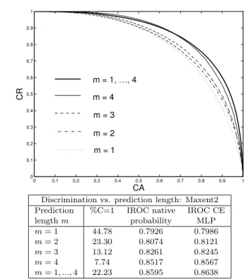
6.2.3 Dealing with predictions of various lengths. We try different approaches for dealing with various length predictions: we train four separate MLPs for fixed length predictions of one, respectively, two, three, or four words. Then we train a unique MLP over predictions with various lengths, ranging from one to four, and compared the results in table X

The best discriminability was obtained by the MLP trained on predictions of various lengths and in all cases the CE-score discriminability is at least as good as the base score (the native probability estimated by the base models).

0 0.1 0.2 0.3 0.4 0.5 0.6 0.7 0.8 0.9 1 0 0.1 0.2 0.3 0.4 0.5 0.6 0.7 0.8 0.9 1 CA CR m = 1 m = 2 m = 3 m = 4 m = 1, …, 4

Discrimination vs. prediction length: Maxent2 Prediction %C=1 IROC native IROC CE length m probability MLP m= 1 44.78 0.7926 0.7986 m= 2 23.30 0.8074 0.8121 m= 3 13.12 0.8261 0.8245 m= 4 7.74 0.8517 0.8567 m= 1, ..., 4 22.23 0.8595 0.8638

Table X. model = Maxent2, nb.of words as m = 1, m = 2, m = 3, m = 4, m = 1, . . . , 4: ROC curve and impact of prediction length on discrimination capacity and accuracy for the Maxent2 prediction model

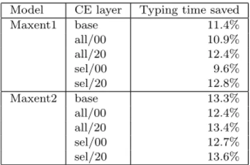
6.2.4 User-Model Evaluations. Evaluations with the user simulation are per-formed only with the Maxent1 and Maxent2 models. The results on a single Hansard file containing 1272 sentence pairs are shown in the table XI. All are generated using the mixed length (1-4 word predictions) neural nets.

According to our experiments, the best performing systems are the ones using the MLPs with 20 hidden units. These systems outperformed the baseline system that used the base model probabilities during the simulation for typing-speed benefit computations. Interestingly, the simpler CE-models with 0 hidden units performed worse than the baseline.

6.2.5 Model Combination. We now describe how various model combination schemes affect prediction accuracy. We use the Bayes and the Maxent2 prediction models: we try to exploit the fact that these two models, being fundamentally dif-ferent, tend to be complementary in some of their responses. Adding the Maxent1 model to the combination would not have yield additional improvements, as Max-ent1 and Maxent2 are too similar. We chose the latter because it has a slightly better prediction accuracy than the first. Our CE models are the corresponding MLPs because they clearly outperform the SLPs. The results presented in table XII are reported on the various length prediction task for up to four words.

Model CE layer Typing time saved Maxent1 base 11.4% all/00 10.9% all/20 12.4% sel/00 9.6% sel/20 12.8% Maxent2 base 13.3% all/00 12.4% all/20 13.4% sel/00 12.7% sel/20 13.6%

Table XI. User simulation results with various CE-layer configurations The base entries are for the base model; all means the full feature sets, sel means selected ones; and the numbers after the slashes describe the hidden units. The results column gives estimated percentage of typing time saved according to the user model.

in parallel and choose one of the proposed prediction hypotheses according to the following voting criteria:

—Maximum CE vote: choose the prediction with the highest CE;

—Maximum native probability vote: choose the prediction with the highest native probability.

As a baseline comparison, we use the accuracy of the individual native prediction models. Then we compute the maximum gain we can expect with an optimal model combination strategy, obtained by running an ”oracle” that always picks the right answer.

The results are positive: the maximum CE voting scheme obtains a 29.31% of the maximum possible accuracy gain over the best of the two individual mod-els (Maxent2). Moreover, if we choose the maximum native probability vote, the overall accuracy actually drops. These results are a strong motivation for our post-prediction confidence estimation approach: by training an additional CE layer using the same confidence features and train data for different underlying prediction mod-els we obtain more uniform estimates of the probability of correctness. Contrary to the native probabilities, the CE probabilities are compatible among the various underlying models and can be used for model combinations.

The combination scheme is very basic and relies on maximum score voting. Other combination schemes (such as stacking Section 3.1) might be more adequate for the task but we wanted to show another possible use of the already defined confidence scores.

We conclude that CE can be successfully used for Transtype: productivity gains can be observed during simulations when confidence score is used for deciding which translation predictions to present to the user, instead of using the base model prob-abilities. Moreover, the CE-based combination scheme, although very simplistic, allow us to combine the results of two independent translation systems exceeding the performance of each individual system.

Model Combination Prediction Accuracy Prediction model combination Accuracy

Bayes alone 8.77

Maxent alone 22.23 Max native probability vote combination 17.49 Max CE vote combination 23.86 Optimal combination 27.79

Table XII. Prediction accuracy of the Bayes and Maxent2 model compared with combined model accuracy

7. DISCUSSION: CE ADVANTAGES AND LIMITATIONS

As described in section 1, confidence measures can either be derived directly from the base system or calculated by a separate CE layer. In this section we compare these two approaches.

Confidence measures that come directly from the base system have the obvious advantage of simplicity, particularly for probabilistic systems where scoring func-tions can be used without modification. Apart from the work needed to create a CE layer itself, effort is also required to produce the necessary training corpus of examples of system output labelled with their correctness status, as discussed in section 4. For some tasks, like machine translation, this corpus is substantially more difficult to produce than the one used to train the base system, which may be already available (eg, a parallel corpus).

A key advantage of using a CE layer is that is a separate module, distinct from the base system. This has several implications:

—Because it specializes in solving the confidence problem, it often gives better results than confidence measures derived directly from the base system, as we have seen in this paper.

—It can incorporate sources of knowledge that may be difficult or inconvenient to add to the base system. These include features like sentence length for MT that are good predictors of confidence but poor predictors of the correct output. Be-cause it is applied in a post-processing step, a CE layer can also model properties of the search algorithm that are inaccessible to the base system.

—The CE layer is smaller and lighter than the base system, and hence easier to adapt to new domains and new users (modulo the availability of correctness data for these contexts).

—It is possible to re-use CE software for different base systems.

The other main advantage to using a CE layer is that it can compute estimates of correctness probabilities P (C = 1|x, y, k). The best alternatives from the base system are posterior probabilities p(y|x), but these are often difficult to extract, and they can be poor estimates. As described in section 2, they are also less useful than correctness probabilities due to the normalization constraint. Correctness probabilities are useful in many contexts:

—In a decision-theoretic setting, probabilities are required in order to calculate the lowest-cost output for a given input.

—When a collection of heterogeneous models is available for some problem, output probabilities provide a principled way of combining them.

—When multiplying conditional probabilities to compute joint distributions, the accuracy of the result is crucially dependent on the stability of the conditional estimates across different contexts. This is important for applications like speech recognition and machine translation that perform searches over a large space of output sentences, represented as sequences of words.

Thus, for many applications, the benefits from using a separate CE layer will justify the extra effort involved.

8. CONCLUSION

We presented CE as a generic machine learning approach for computing confidence measures for improving an NLP application. CE can be used if relevant confidence features are found, if reliable automatic evaluation methods of the base NLP tech-nology exist and if large annotated corpora are available for training and testing the CE models.

Applications benefit from a light CE-layer when the base application is fixed. If potential base-model accuracy improvements are poor, the additional data is more useful in practice for improving discriminability and removing wrong outputs. We showed that the probabilities of correctness estimated by the CE layer exceed the original probabilities in discrimination capacity.

CE can be used to combine results from different applications. In our MT ap-plication, a model combination based on a maximum CE voting scheme yielded a 29.31% accuracy improvement in maximum accuracy gain. A similar voting scheme using the native probabilities decreased the accuracy of the model combination.

Prediction accuracy was not an important factor for determining the discrimina-tion capacity of the confidence estimate. However, the original probability estima-tion was the most relevant confidence feature in most of our experiments.

We experimented with multi-layer perceptrons (MLPs) with 0 (similar to Maxent models) and up to 20 hidden units. Results varied with the amount of data available and the task, but overall, the use of a hidden units improved the performance.

We intend to continue experimenting further with CE on other SMT systems for other NLP tasks, such as language identification or parsing.

ACKNOWLEDGMENT

The authors wish to thank Didier Guillevic and Yves Normandin for their con-tribution in providing the experimental results regarding the ASR application we presented. We wish to thank the members of th RALI laboratory for their support and advice, in particular Elliott Macklovitch and Philippe Langlais.

REFERENCES

Bishop, C. M.1995. Neural Networks for Pattern Recognition. Oxford University Press, Oxford. Blatz, J., Fitzgerald, E., Foster, G., Gandrabur, S., Goutte, C., Kulesza, A., Sanchis, A., and Ueffing, N. 2004a. Confidence estimation for machine translation. Tech. rep., Final report JHU / CLSP 2003 Summer Workshop, Baltimore.