Sensitivity Study of Regional Climate Model Simulations to Large-Scale
Nudging Parameters
ADELINAALEXANDRU
Canadian Network for Regional Climate Modelling and Diagnostics, and Centre ESCER, Universite´ du Que´bec, Montreal, Que´bec, Canada
RAMON DEELIA
Canadian Network for Regional Climate Modelling and Diagnostics, and Centre ESCER, Universite´ du Que´bec, and Ouranos Consortium, Montreal, Que´bec, Canada
RENE´ LAPRISE ANDLEOSEPAROVIC
Canadian Network for Regional Climate Modelling and Diagnostics, and Centre ESCER, Universite´ du Que´bec, Montreal, Que´bec, Canada
SE´ BASTIENBINER
Ouranos Consortium, Montreal, Que´bec, Canada (Manuscript received 11 April 2008, in final form 29 August 2008)
ABSTRACT
Previous studies with nested regional climate models (RCMs) have shown that large-scale spectral nudging (SN) seems to be a powerful method to correct RCMs’ weaknesses such as internal variability, intermittent divergence in phase space (IDPS), and simulated climate dependence on domain size and geometry. Despite its initial success, SN is not yet in widespread use because of disagreement regarding the main premises—the unconfirmed advantages of removing freedom from RCMs’ large scales—and lingering doubts regarding its potentially negative side effects. This research addresses the latter issue. Five experiments have been carried out with the Canadian RCM (CRCM) over North America. Each experiment, performed under a given SN configuration, consists of four ensembles of simulations integrated on four different domain sizes for a summer season. In each experiment, the effects of SN on internal variability, time means, extremes, and power spectra are discussed. As anticipated from previous investigations, the present study confirms that internal variability, as well as simulated-climate dependence on domain size, decreases with increased SN strength. Our results further indicate a noticeable reduction of precipitation extremes as well as low-level vorticity amplitude in almost all length scales, as a side effect of SN; these effects are mostly perceived when SN is the most intense. Overall results indicate that the use of a weak to mild SN may constitute a reasonable compromise between the risk of decoupling of the RCM internal solution from the lateral boundary con-ditions (when using large domains without SN) and an excessive control of the large scales (with strong SN).
1. Introduction
Regional climate models (RCMs) are one-way nested limited-area models that are used to downscale
low-resolution atmospheric information, usually reanalyses or (general circulation model) GCM-simulated data (e.g., Giorgi 1990; Christensen et al. 2007). Although the ap-plication of lateral boundary conditions (LBC) con-strains RCMs’ simulations, the dynamical formulation and physical parameterizations of RCMs are as non-linear as those of any GCM, and thus, nested models may exhibit a certain level of freedom and chaotic be-havior in their simulations. This freedom is ultimately responsible for the additional information generated by Corresponding author address: Adelina Alexandru,
De´parte-ment des Sciences de la Terre et de l’Atmosphe`re, UQAM-Ouranos, 550 rue Sherbrooke Ouest, 19e e´tage, Tour Ouest, Montreal, QC H3A 1B9, Canada.
E-mail: [email protected]
1666 M O N T H L Y W E A T H E R R E V I E W VOLUME137
DOI: 10.1175/2008MWR2620.1
RCMs, but it also promotes the manifestation of inter-nal variability (IV). This IV is here defined as the ca-pacity of a given RCM, driven by the same set of LBC, to produce different solutions (e.g., Ji and Vernekar 1997; Vernekar and Ji 1999; Rinke and Dethloff 2000; Weisse et al. 2000; Weisse and Feser 2003; von Storch 2005; Alexandru et al. 2007). In practice, IV is found to vary as a function of season, domain size, and geo-graphical location (e.g., Seth and Giorgi 1998; Giorgi and Bi 2000; Christensen et al. 2001; Caya and Biner 2004; Rinke et al. 2004; Lucas-Picher et al. 2004; Castro et al. 2005; Alexandru et al. 2007). Recent findings on IV have also shown a noteworthy impact on seasonal average statistics (Alexandru et al. 2007).
While many properties of IV are now fairly well un-derstood, there is some disagreement in the modeling community as to how IV should be considered: as an undesirable feature of nested models simulations, which should be eliminated or reduced as much as possible (since it creates an artificial variability whose main role is to convolute experiment design and data analysis), or whether nested model freedom is necessary to obtain the best performance. There is also the possibility that both too little and too much IV is to be avoided.
The basic hypothesis behind the nesting strategy is that an RCM will produce realistic finescale details, which represent RCM’s potential added value, over a region by being fed by large-scale low-resolution data at its lateral boundaries. Another hypothesis, although more controversial, is that RCM-simulated large-scale circulation should remain similar to its driving coun-terpart at all times. Studies performed with RCMs using the classic lateral boundary driving strategy (Davies 1976) have shown that the latter assumption is not al-ways fulfilled; the sole control of the boundaries is not sufficient to prevent some decorrelation of the RCM-simulated fields with the driving ones for length scales larger than 1500 km (e.g., Riette and Caya 2002). In this way, RCMs may intermittently generate their own large-scale circulation that diverges significantly from that prescribed at the boundaries (e.g., Rinke and Dethloff 2000; Weisse and Feser 2003; Miguez-Macho et al. 2004). One way to mitigate this intermittent divergence in phase space (e.g., Weisse and Feser 2003) is to force the large scales not only at the lateral boundaries but also within the domain. The technique of large-scale spectral nudging (SN; e.g., Waldron et al. 1996; von Storch et al. 2000) adds nudging terms to the model equations. The nudging terms are designed to have maximum efficiency for large scales without affecting the small scales, thus ensuring that the RCM large-scale solution remains close to the large-scale forcing. The SN should not, in principle, impede the ability of the RCM to develop
regional and small-scale features superimposed on the large-scale driving conditions (e.g., von Storch et al. 2000; Biner et al. 2000). In addition, the SN is usually confined to the upper levels of an RCM, and hence the simulation in the lower troposphere remains fairly free. The SN technique has been implemented in a number of RCMs (e.g., Kida et al. 1991; Sasaki et al. 1995; McGregor et al. 1998; von Storch et al. 2000; Biner et al. 2000; Riette and Caya 2002) and many studies have been performed to assess strengths of the technique. The study of Miguez-Macho et al. (2005) showed that sig-nificant errors in the monthly precipitation pattern (June 2000) for a domain over North America was largely due to a systematic distortion of the large-scale flow interacting with the lateral boundaries. As a solu-tion for the boundary problem, they found that SN could eliminate the bias in the circulation and produce a much improved precipitation pattern. In a previous study, Miguez-Macho et al. (2004) had shown that SN also reduced the sensitivity of regional precipitation patterns to the choice of model domain and grid geo-metry, while maintaining the RCM-simulated small-scale structures. Meinke et al. (2006) showed a better agreement of simulated cloudiness with satellite-derived observations with SN. The study of Weisse and Feser (2003) demonstrated that intermittent divergence in phase space is strongly reduced by the use of SN.
The present study examines the impact of various SN configurations on CRCM simulations. The objective is to determine whether there are any secondary effects from the application of SN such as a possible reduction of the model’s ability to develop small-scale features. A broad series of CRCM experiments is carried out over North America with different SN configurations; each experiment consists of ensembles of 15 runs for 4 different domain sizes. To evaluate the effects of an extreme nudging, one experiment was carried out nudging the CRCM with the maximum strength of the SN—equivalent to a replacement of the largest waves—at all levels.
The paper is organized as follows. Section 2 briefly describes the simulation setup and evaluation methods used for the experiments. Section 3 examines the impact of SN on the IV (section 3a), on the ensemble mean (section 3b), on precipitation extremes (section 3c), and on power spectra (section 3d). Concluding remarks are presented in section 4.
2. The CRCM and experimental design a. Model description
The model used in the present study is version 3.6.1 of the Canadian RCM (CRCM; Caya and Laprise 1999).
The CRCM is a limited-area model based on the fully compressible Euler equations solved by a semi-implicit and semi-Lagrangian marching scheme (Bergeron et al. 1994; Laprise et al. 1997). The model uses the physical parameterization package of the second-generation CGCM (GCMii; McFarlane et al. 1992) except for the Bechtold–Kain–Fritsch deep and shallow convec-tive parameterization (Kain and Fritsch 1990; Bechtold et al. 2001). The computational points are fixed on a three-dimensional staggered grid projected onto polar-stereographic coordinates in the horizontal and Gal-Chen terrain-following levels in the vertical (Gal-Gal-Chen and Somerville 1975).
To define the initial conditions (ICs), the CRCM re-quires information about the following atmospheric fields: horizontal winds, vertical motion, temperature, surface pressure, and specific humidity. These atmo-spheric fields are also required at each time step to de-fine the LBC. Nudging is also applied on the horizontal wind components over a 10 gridpoint sponge zone near the lateral boundary where the CRCM-simulated winds are relaxed toward the values of the driving data (Davies 1976). The necessary atmospheric IC and LBC are pro-vided by linear interpolation of the National Centers for Environmental Prediction–National Center for Atmo-spheric Research (NCEP–NCAR) reanalysis data avail-able each 6 h (Kalnay et al. 1996). In addition, the CRCM requires IC for the following land surface variables: ground temperature, liquid and frozen soil water frac-tion, and snow amount and snow age. Ocean-surface variables are prescribed from Atmospheric Model In-tercomparison Project (AMIP) data (Fiorino 1997). b. Large-scale spectral nudging
In the CRCM, there is an option for SN, in addition to the standard Davies LBC treatment. The current CRCM SN technique, documented by Riette and Caya (2002), closely follows the approach of von Storch et al. (2000), but it uses a scale decomposition based on the discrete cosine transform (DCT) implemented by Denis et al. (2002). There are three adjustable parameters to CRCM SN: the length scale beyond which SN is applied, the maximum strength of the SN (}max), and the lowest
model level (L0) below which no SN is applied. The SN
strength } (defined as the fraction of CRCM field that is replaced by the reanalyses at each time step) is taken to vary linearly from 0 (corresponding to L0) to }max(at
the uppermost model level). The SN can be applied to any model variable; in this study, it is applied to the horizontal wind components only. Some early experi-ments have shown that the use of additional variables such as the mass field does not make a substantial dif-ference (see Riette and Caya 2002), and this
configu-ration has been applied routinely in later versions of this model (see de Elı´a et al. 2008). Figure 1 shows the vari-ous profiles of SN used in this paper.
c. Simulation setup
Figure 2 identifies the various domains and topogra-phy used for the 45-km grid mesh CRCM simulations for this study. Four model domains with sizes of 140 3 140, 120 3 120, 100 3 100, and 80 3 80 grid points cover eastern North America and part of the Atlantic Ocean for the summer of 1993. The position of the domain aims mostly at having a relatively flat topogra-phy in order to simplify the interpretation of the study. The choice of season is due to our interest to confront large internal variability episodes. In addition, this com-bination of domain and season has previously been studied several times (Alexandru et al. 2007; Lucas-Picher et al. 2008). Given the important role of the convection in the southern United States in triggering IV (Alexandru et al. 2007), the four domains are defined keeping the southwest corner fixed. The CRCM uses a 15-min time step and 18 Gal-Chen levels in the vertical, with a model lid at 30 km.
Five experiments are carried out to test the sensitivity of CRCM simulations to the variation of the SN pa-rameters. Of the three parameters controlling the SN, only two will be studied here. The one left out, the length scale beyond which SN is applied, will be kept fix at 1400 km (scales larger than 1400 km are nudged, this value being chosen because information content in the reanalyses drops for shorter wavelengths, as shown by Separovic et al. 2008). The reasons for not study the sensitivity of this parameter are that first, preliminary studies varying it did not show very high sensitivity, and second, the computational cost. There are 280 three-month simulations involved in this research.
The experiments, performed for different configura-tions of SN, consist of ensembles of several members (generally 15) generated for 4 different domain sizes. One experiment is performed without SN (}max50);
three experiments are made with the same }max50.05
but different L0(500, 700, and 850 hPa); a fifth
experi-ment is performed with a uniform value of } 5 }max5
1 at all model levels. In this full SN case, the large scales of the CRCM are entirely replaced by those of the re-analyses, at all levels from the surface to the model lid (see Fig. 1); due to the particularly weak IV, only 10-member ensembles are integrated in the full SN ex-periment. The five experiments are summarized in Table 1. All integrations from each ensemble were initialized 1 day apart, starting the 0000 UTC 5 May 1993 up to the 0000 UTC 20 May 1993; all simulations end on 0000 UTC 1 September 1993, so that all ensemble members
for different domain sizes overlap for the full three months of June–July–August 1993, with a spinup period varying from 11 to 25 days. The integrations share ex-actly the same LBC for atmospheric fields and the same prescribed SST and sea ice coverage for the ocean sur-face.
d. Evaluation methods
The IV of the model will be estimated by measuring the spread among the ensemble members during the integration period, using the standard deviation ( ffiffiffiffiffiffiffis2
en
p ) between the 15 members, where sen2 is the variance
defined as s2en(i, j, k, t) 5 1 M 1
å
M m51 [Xm(i, j, k, t) ÆXæ(i, j, k, t)]2. (1) The term Xm(i, j, k, t) refers to the value of a variable Xat grid point (i, j) on level k at time t for member m in the ensemble and M is the total number of ensemble members (15 or 10, depending on the experiment). The term ÆXæ(i, j, k, t) is the ensemble mean defined as
ÆXæ(i, j, k, t) 5 1
M
å
M
m51
Xm(i, j, k, t). (2)
In our evaluations regarding the ensemble mean, we also use the following:
d the 3-month time average of the ensemble mean
(seasonal mean of the ensemble mean) defined as
ÆXæt(i, j, k) 5 1
N
å
N
t51
ÆXæ(i, j, k, t), (3)
where N refers to the number of archived 6-hourly time steps in the period of interest (N 5 369 time steps for three summer months), and
d the domain average of the ensemble mean, defined as
ÆXæxy(k, t) 5 1 I 3 j
å
J j51å
I I51 ÆXæ(i, j, k, t), (4)where I and J are the number of grid points along the x and y directions over the domain of interest. A measure of the domain-averaged IV during the course of the model integration is provided by the square root of the spatially averaged variance ( ffiffiffiffiffiffiffiffiffiffiffis2
en xy q ), where s2 en xy is computed as s2 en xy (k, t) 5 1 I 3 J
å
J j51å
I i51 s2en(i, j, k, t). (5)The 3-month time average of IV and its spatial dis-tribution in the domain is provided by the square root of the time-averaged variance ( ffiffiffiffiffiffiffiffiffis2
en t q ), where s2 en t is de-fined as s2 en t (i, j, k) 5 1 N
å
N t51 s2en(i, j, k, t). (6) FIG. 1. The five CRCM SN experiments.We also use in our evaluations spatially averaged time-averaged IV defined as the square root of the domain-averaged time-domain-averaged variance ffiffiffiffiffiffiffiffiffiffiffiffi
s2 en txy r , where s2 en txy is provided by s2 en txy (k) 5 1 I 3 J 3 N
å
J j51å
I i51å
N t51 s2en(i, j, k, t). (7)The influence of internal variability at the seasonal scale is appreciated by the variation of the seasonal-mean field. The spread between seasonal averages of the ensemble members is estimated as the square root of the variance between individual member seasonal averages ( ffiffiffiffiffis2 s p ), where s2sis computed as s2s(i, j, k) 5 1 M
å
M m51 [Xm t (i, j, k) ÆXæt(i, j, k)]2, (8) where Xm t(i, j, k) is the seasonal average of member m, and ÆXæt(i, j, k) is the seasonal average of the ensemble mean. The s2swill be referred as internal variability of
the seasonal mean (IVs).
A measure of the domain-averaged IVs is provided by s2 s xy (k) 5 1 I 3 J
å
J j51å
I i51 s2en(i, j, k). (9)The relative importance of internal variability on the seasonal mean is provided by the coefficient of variation (I) computed as
TABLE1. Synthesis of the experiments performed.
Test expt P0 (hPa) amax (%) No. of ensembles Domain size 500-hPa SN 500 0.05 4 140 3 140 120 3 120 100 3 100 80 3 80 700-hPa SN 700 0.05 4 140 3 140 120 3 120 100 3 100 80 3 80 850-hPa SN 850 0.05 4 140 3 140 120 3 120 100 3 100 80 3 80 Full SN 1000 1 4 140 3 140 120 3 120 100 3 100 80 3 80 FIG. 2. CRCM computational domains and topography.
I(i, j, k) 5 ffiffiffiffiffiffiffiffiffiffiffiffiffiffiffiffiffiffiffi s2 s(i, j, k) p ÆXæt(i, j, k) . (10)
This measure will be particularly useful for the precip-itation field.
These statistics will be evaluated excluding the spinup period and removing the 10-point relaxation zone. The study will focus on precipitation and 850-hPa geo-potential height.
To reveal the behavior of the simulations for dif-ferent length scales, we have applied a spectral analysis to the simulated datasets. The separation of scales is performed utilizing the two-dimensional DCT, intro-duced in the analysis of meteorological fields by Denis et al. (2002). The particularities of this tool can be found in the aforementioned paper, and for an appli-cation similar to that of this research see Separovic et al. (2008).
The effect of the spectral nudging is going to be measured with respect to a control run—the unnudged simulation—and, in some cases, also with respect to observations. This version of the CRCM has relatively good ability to reproduce the present climate but tends to overestimate precipitation almost everywhere, and particularly during convective events (Paquin et al. 2002). Under this condition, we believe that closeness to observed precipitation could be a highly misleading score, and hence will not be used in this study.
3. Analysis of the results
In this section we will examine the impact of SN on the IV (section 3a), on the ensemble mean (section 3b), on precipitation extremes (section 3c), and on power spectra (section 3d).
a. The influence of SN on IV
We begin by showing specific cases illustrating the effect of SN on the IV. Figure 3 presents four particular instances (four rows) of the 850-hPa geopotential height field as simulated by CRCM on the 120 3 120 domain with different SN configurations (first four columns). The last column on the right shows the NCEP–NCAR reanalysis. Only five members of the ensemble are shown for clarity. The case of full nudging is not shown due to the similarities of the simulations with NCEP–NCAR.
In the first case (top row), corresponding to 0000 UTC 25 July 1993, the CRCM without SN exhibits different solutions in the middle of the domain as a manifestation of the IV of the model. This particular case was dis-cussed in detail by Alexandru et al. (2007). The pro-gressive increase of SN reduces differences between
simulations and, consequently, the IV, and strengthens, as expected, the similarities with the driving fields. This result corresponds with the intuition developed in the recent years following the work of Weisse and Feser (2003). Model response to SN, however, is not always this straightforward. The middle panels of Fig. 3 show that IV sometimes increases with SN; this is particularly clear for the 500- and 700-hPa SN. The fourth case (lowest row), corresponding to 0000 UTC 28 June 1993, shows significant changes in the simulated patterns for larger vertical extents of SN: the low pressure system near North Carolina and Virginia disappears when the SN is significantly increased. This case also exhibits, counter intuitively, a notable increase in IV when passing from 500- to 700-hPa SN.
Figure 4 depicts the time series of domain-averaged IV ( ffiffiffiffiffiffiffiffiffiffiffis2
en xy
q
) [as defined in (5)] for precipitation (left column) and 850-hPa geopotential (right column), for five configurations of SN (on separate rows) and four domain sizes (lines of different colors). Without SN (Figs. 4a,b), the results with the largest domain (140 3 140) have little in common with those obtained with smaller domains, showing much larger peaks of IV that are temporally decorrelated from those of smaller do-mains. Even the weaker 500-hPa SN (Figs. 4c,d) is ef-fective in reducing the differences between the time series and improving their temporal correlation, with the most significant impact for the largest 140 3 140 domain. The 500- and 700-hPa SN had the effect of in-creasing the IV for the 120 3 120 domain near step 100 (marked by the red arrow), although, as noted earlier, there is a decrease of IV on average with increasing SN strength. Further increase of SN reduces IV and pro-duces a convergence of the time evolution of IV be-tween the ensembles on different domain sizes. It is noteworthy that some IV remains even with application of full SN; this could be related to the fact that the active convection in the South of the continental United States is partially independent of the large scale.
Figure 5 illustrates the 3-month time-averaged IV ( ffiffiffiffiffiffiffiffiffis2
en t
q
) [as defined in (6)] for precipitation (Fig. 5a) and the 850-hPa geopotential height (Fig. 5b) for different SN. The ensemble without SN shows a clear depen-dence of IV on domain size, as noted before by Alex-andru et al. (2007). In general, the larger domain sizes exhibit a larger IV; this is particularly obvious for the 850-hPa geopotential height (Fig. 5b). There are, how-ever, local exceptions to this general rule; for example, the intense IV maximum of precipitation near the southeast corner of the 100 3 100 domain is absent or weaker in ensembles with larger domain sizes; a com-parison to observation data shows that the model overestimates the precipitation in that particular area
on the 100 3 100 domain, creating a wider precipitation area with higher intensity of IV. Study shows that in-creased SN reduces this sensitivity of IV to domain size and almost suppresses it by a full SN. Furthermore, for a given domain size, the time-averaged IV is reduced by increasing the SN, and this is particularly true for the larger domain sizes; an exception to this general IV decreasing tendency with SN, can be noticed near the southeast corner of the 100 3 100 domain (mentioned above), where the IV has a more intense maximum for
the 500-hPa SN than without SN. It is worth noting that even the case of full SN shows a nonnegligible IV in the southeast United States. (As can be seen in Fig. 10a, this area coincides with a region of large amounts of pre-cipitation, mostly of convective origin.)
b. The influence of SN on the ensemble mean The influence of the SN on the internal variability of the seasonal mean [IVS; defined as ffiffiffiffiffis2
s
p
in (8)] is shown in Fig. 6 for the precipitation (Fig. 6a) and the 850-hPa FIG. 3. (a),(b),(c),(d) Four cases of five CRCM runs (different colors) with a delay of 24 h in their IC performed in different model configurations (first four columns) for the 850-hPa geopotential height (dam); the last column shows NCEP–NCAR corresponding to the four cases.
FIG. 4. Four time series of domain-averaged IV corresponding to the four domains [140 3 140 (blue), 120 3 120 (red), 100 3 100 (green), and 80 3 80 (dark blue)] for (left) precipitation and (right) the 850-hPa geopotential height in different model configurations.
geopotential height (Fig. 6b). In general, as for IV, the IVS tends to decrease with increasing SN, more signif-icantly for the geopotential height on the largest do-main, where IVS values are considerably lower even
with the weak 500-hPa SN (Fig. 6b). As expected, the IVS reaches its smallest values, for both variables, in the full SN case with a negligible sensitivity to domain size. For the precipitation with 500-hPa SN (Fig. 6a), it is FIG. 5. (a) Precipitation time-average IV on four different domain sizes (four columns) for five different model configurations (five rows). (b) 850-hPa geopotential height time-average internal variability on four different domain sizes (four columns) for five different model configurations (five rows).
worth noting an increased IVS in the southeast corner of the 100 3 100 domain (as discussed in the above para-graph for the IV); the coefficient of variation (I) [as defined in (10)] is around 42%, significantly larger than in the case without SN (22%).
Figure 7 summarizes the previous results by showing, for both variables, the variation of the domain-averaged time-averaged IV ( ffiffiffiffiffiffiffiffiffiffiffiffi s2 en txy r
) [as defined in (7)] (Fig. 7, left panels) and of the domain-averaged IVS ( sffiffiffiffiffiffiffiffiffi2
s xy
q
) [as defined in (9)] (Fig. 7, right panels) with the domain size FIG. 5. (Continued)
FIG. 6. (a) IV of precipitation seasonal mean on four different domain sizes (four columns) for five different model con-figurations (five rows). (b) Internal variability of 850-hPa geopotential height seasonal mean on four different domain sizes (four columns) for five different model configurations (five rows).
for different SN configurations. Our results confirm those found by Weisse and Feser (2003) regarding the ability of SN to reduce the IV on average. As was dis-cussed by de Elia et al. (2008) and Lucas-Picher et al. (2008), it is interesting to note that internal variability of the instantaneous departures (IV) and those of seasonal
departures (IVS) display similar behavior safe, ap-proximately, a multiplicative constant. Figure 7 also shows that IV can be reduced on average, either by increasing SN strength or by reducing domain size. It is also interesting to note the reduction of domain size dependence as the vertical extent of the SN increases. It FIG. 6. (Continued)
is also clear that without SN, an increase of domain size from 120 3 120 to 140 3 140 introduces a major increase in IV. This major jump in IV dependence on domain size was obtained, it is worth recalling, with a single summer season. Although additional research is needed to confirm this nonlinear tendency, this result may suggests that domains this large may need more control than the one usually provided at the boundary, and that SN seems to offer a solution.
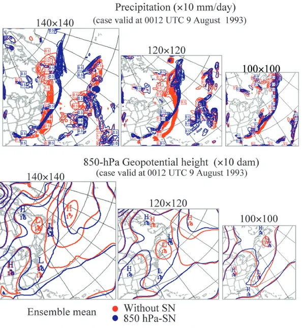
After analyzing the spread between members in the ensembles (which we termed IV) and the spread be-tween seasonal means of the members in the ensem-bles (which we termed IVS), we now concentrate on a particular case (0012 UTC 9 August 1993) and study the effect of SN strength on the ensemble mean of different domain sizes. Figure 8 depicts, for the three larger domain sizes, the ensemble means in two model configurations—no SN and 850-hPa SN—for precipi-tation (top panels) and 850-hPa geopotential height (bottom panels). It can be seen that the impact of SN on ensemble means is quite pronounced for the 140 3 140 domain and more reduced for the smaller 100 3 100 domain.
The fact that the ensemble averages for different model configurations show differences in the phase of the weather system implies that these errors are not
solely a consequence of IV. Thus, the random error originated by the IV is removed by ensemble averaging, and hence only the systematic bias should remain. One of the main hypotheses of regional climate modeling is that errors in the phase of particular weather systems are not an important issue, but this is only true if this bias is not reflected in the time average.
The present study also reveals an effect of SN on bi-modalities that are sometimes noted in ensembles. For the largest domains, where the impact of SN is the largest, a difference has been noted between the results without SN (Alexandru et al. 2007) and those with SN concerning bimodal behavior of the ensemble. For the case without SN, the 15 members appear to separate into a group of 5 members producing a low pressure system over the ocean, close to the Canadian Atlantic region, and another group of 10 members showing a high pressure system over the same area and an intense precipitation trough close to the U.S. East Coast (Fig. 9a; see Alexandru et al. 2007). We now see that when the degree of SN applied to the model is progressively increased (Fig. 9b), the effect is to foster the develop-ment of the solution that is closest to the observed data; in this particular case, this solution happens to corre-spond to the group with the smallest number of mem-bers, as shown in Fig. 9c.
FIG. 7. Domain-averaged time-averaged internal variability for (top) precipitation and (bottom) 850-hPa geopotential height in different model configurations [without SN (mauve), 500-hPa SN (green), 700-hPa SN (dark blue), 850-hPa SN (black), and full SN (red)]. For all four domains, the statistics are evaluated over a common area whose size corresponds to that of the smallest domain.
Figure 10 illustrates seasonal averages of the ensem-ble means corresponding to the four domain sizes (four columns) for different SN configurations (five rows) for the precipitation (Fig. 10a) and 850-hPa geopotential height (Fig. 10b). The use of 3-month time average and 15-member ensemble mean makes this average statis-tically quite robust and, accordingly, most salient dif-ferences are significant. Most fields show little differ-ences in mean for the various domains and SN. A close inspection, however, reveals occasional differences for those simulations performed with no or weak SN: for example, the seasonal average precipitation increases over eastern Tennessee as the domain size is reduced, as
noted by Alexandru et al. (2007) for the simulations without SN. Some details are particularly robust against variations of domain sizes, such as the minimum pre-cipitation over Ohio. In the case of full SN, however, the precipitation minimum in Ohio is particularly low, and precipitation is also reduced over Georgia and the At-lantic Ocean. There are also some areas such as Mis-sissippi where precipitation is increased with full SN; this is rather counterintuitive, as one may have expected that removing degrees of freedom by SN may imply suppression of small-scale development, especially so close to the inflow region of the regional domain. It is also interesting to note the disappearance of the storm FIG. 8. Ensemble means in two model configurations—without SN (red) and 850-hPa SN (blue)—on different domain
track over the ocean for the smallest domain, and its declining in the full SN configuration.
Figure 10b shows, for all four domains, the seasonal averages of the ensemble means from all SN configu-rations against the NCEP–NCAR reanalysis for the 850-hPa geopotential height. For the largest domain (140 3 140), there are significant similarities between
500-, 700-, and 850-hPa SN seasonal ensemble means and some deviations with either full SN or no SN; striking deviations are noticed with NCEP–NCAR on the largest domain. With a domain size of 120 3 120, the deviations are reduced, and with yet smaller domain sizes, the differences become negligible. It is worth noting the effect of domain size reduction in approaching FIG. 9. Domain 140 3 140: (a) 850-hPa geopotential height bimodal solution, (b) 15 runs of 850-hPa geopotential
height in 850-hPa SN, and (c) 850-hPa geopotential height in NCEP–NCAR.
the regional model simulation to its driving data on the smaller domains, as well as, the small impact that SN might have for small domains.
Previous experiences with this CRCM version have shown a good ability to reproduce the geopotential fields, surface temperature, and other variables, but a tendency to overestimate precipitation of the convec-tive type over land. This effect is particularly dominant during summer almost everywhere (see Paquin et al. 2002; Laprise et al. 2003; Plummer et al. 2006; de Elia et al. 2008). For this reason, comparison against ob-served mean precipitation is not discussed.
c. The influence of SN on precipitation extremes Figure 11 shows the largest amounts of 6-hourly cu-mulative precipitation over the domain during the model integration (henceforth called domain precipitation ex-tremes) simulated by each of the ensemble members (lines of different colors) in different SN configurations (four panels). We note that, for the runs without SN on the 140 3 140 domain, the largest extremes occur from 10 to 15 July, associated with the intense precipitation trough given by the group of 10 simulations in the bi-modal behavior of the ensemble, as discussed in section 3b. The magnitude of this maximum is progressively attenuated as the degree of SN is progressively in-creased (the top four panels of Fig. 11). Similar behavior is noted for the 120 3 120 domain; precipitation ex-tremes decrease in number and intensity as the degree of SN is progressively increased (bottom row of Fig. 11).
d. The influence of SN on power spectra
In this section a spectral analysis of the simulations discussed in the previous sections is carried out. A spec-trum is computed over the 80 3 80 gridpoint common area of all the domains involved (minus the relaxa-tion zone), for the particular field of 850-hPa rela-tive vorticity, at each archived 6-h interval. To sum-marize the information we will limit ourselves to time averages and ensemble averages for certain SN config-urations.
Figure 12a shows the time and ensemble average of the spectral power for relative vorticity at 850 hPa for the simulation performed without SN on the 120 3 120 domain. This double averaging implies that 369 con-secutives spectra for each archived time has been av-eraged, and this procedure has been repeated for all 15 members (in the case of the configuration with full SN, the ensemble amounts to 10 members).
To establish the impact of different SN configurations, we have analyzed and compared the power spectra of various simulations. Figure 12b shows the power spectra
of some of the SN configurations already discussed. To gain in visual clarity we present the spectral power of each configuration normalized by that without SN on the 120 3 120 domain (shown in Fig. 12a). This simu-lation will serve as a kind of control configuration, which appears as a black solid horizontal line at 100. The red line shows that the 140 3 140 domain without SN generates more spectral power at all scales, but espe-cially at the largest scales. This result is consistent with the findings of Separovic et al. (2008), which found ex-cess spatial variance in the lower troposphere for this same model version when it is not well constrained by the driving data. An additional factor could be, as shown by Leduc and Laprise (2008), that bigger do-mains allow for more space and time to develop small scales. Reduction of domain size from 120 3 120 to 100 3 100 in a configuration without SN does not have much impact on the spectral power distribution. Vari-ations around the horizontal line may be due to the lack of robustness of the estimation, despite the use of a double averaging. As was the case of IV in Fig. 5a, a change of domain size from 120 3 120 to 140 3 140 seems to have a much larger impact than a reduction from 120 3 120 to 100 3 100.
In addition to variations in domain size, modifica-tions in SN configuramodifica-tions are also evaluated. Black dashed and dotted lines depict the effect of increasing SN extent in a 120 3 120 domain. The results with 500-hPa SN show little difference with respect to those without SN, with the exception of the longest wavelengths. As was shown in Separovic et al. (2008), long wave-lengths at this level tend to be overestimated in CRCM simulations, and SN reduces this overestimation. The configuration with 850-hPa SN shows a decrease in spectral variance in all wavelengths excepting the 200– 400-km range where it is comparable with the configu-ration without SN. When full SN is applied, a very im-portant decrease in spectral variance affects all wave-lengths.
It is important to recall that the choice of the case without SN as control is arbitrary, and hence Fig. 12b does not indicate which one has the correct amount of spectral variance.
4. Conclusions
In the present paper we have tested the impact of large-scale spectral nudging (SN) on ensemble simula-tions performed with the Canadian Regional Climate Model (CRCM). To this end, several experiments using a common simulation setup consisting of four multi-member ensembles integrated on different domain sizes, were performed under five different SN configurations,
FIG. 10. (a) Seasonal ensemble mean on all domains (four columns) in different model configurations (five rows) for the precipitation (mm day21). (b) Seasonal ensemble means from different SN configurations [without SN (blue), 500-hPa SN (red), 700-hPa SN (green), 850-hPa SN (dark blue), and full SN (mauve)] against NCEP–NCAR on all domains for the 850-hPa geopotential height.
for a single summer season over the East Coast of North America. In all experiments, all members of the ensem-ble were initialized at a 1-day interval and were driven by the same set of time-dependent lateral boundary condi-tions taken from NCEP–NCAR reanalyses with pre-scribed sea surface temperatures. The difference be-tween these experiments is the vertical profile and in-tensity of large-scale SN, including one experiment without any SN.
The SN concept deviates from the classical nesting approach by prescribing the forcing not only at the lateral boundaries but also inside the domain for the largest spatial scales. Our results confirm that SN is ef-fective in decreasing the IV of the simulations, and this is particularly the case for the larger 140 3 140 domain. Smaller domains exhibit less IV and are less affected by the use of SN. It has also been shown that with a more intense nudging, IV becomes nearly independent of domain size. It should be kept in mind that these gen-eralizations are less valid for instantaneous cases: it was shown that, for particular time periods, exceptions to these rules do exist. As mentioned in the introduction, it is still unclear to what extent this reduction is a positive or even desired feature. We believe that the answer to this point is dependent on the existence of side effects caused by this reduction, and we devoted the rest of our research to this quest.
It is interesting to note that the application of full SN—replacing entirely the large scales of the model wind field from those of the driving NCEP–NCAR data—still leaves some room for freedom in the simu-lated small scales. In general, this activity was shown to be mostly located in the area with abundant convective precipitation.
Results regarding the time average of precipitation and 850-hPa geopotential height ensemble mean have shown some geographical variation in particular areas when no or weak SN is applied. Experiments have also shown that the ensemble mean is not significantly af-fected by the application of SN for the smallest domains studied. This suggests that Davies’s (1976) control may be just as effective as SN for small domains. We have also noticed that for stronger SN, there is little variation of the ensemble mean as a function of domain size. Thus, similar results may be obtained by employing large SN regardless of the domain size or, alternatively, by avoiding SN when working with small domains.
Results concerning a moderate sensitivity of the av-erage to SN intensity are of considerable importance. Even the case of the extreme SN—the full replacement of the model large scales for those of the driving data— does not suffer a dramatic reduction of average precipi-tation; this suggests that, despite the artificiality intro-duced in the momentum equations by the SN terms, climate still remains fairly realistic. It should be noted, however, that region, season, and even CRCM version are clearly dominated by convective activity and hence the dynamic impact of SN may be underestimated.
The present study also yields some insight into the effect of SN on bimodalities that are sometimes noted in ensembles. For the largest domains, a difference has been noted between the results without SN (Alexandru et al. 2007) and those with SN. In the latter case, as the strength of SN is progressively increased, the effect is to foster the development of the solution closest to the driving data.
At first glance, it may seem that the decrease in pre-cipitation maxima for the case of increased SN is evi-dence of negative effects on small scales, given that FIG. 10. (Continued)
precipitation maxima are often related to small-scale disturbances. Because of the well-documented tendency of the CRCM to underestimate precipitation maxima (e.g., Mailhot et al. 2007), any setup change that reduces precipitation maxima suggests a degradation of the simulation. However, more work is needed to confirm if
reduction of precipitation maxima is a characteristic of SN or just a particularity of our simulations. In addition, the question of whether SN is eventually beneficial or detrimental for the simulations is still open.
Our results confirm, in general, most of the conclu-sions presented in other studies regarding the potential
FIG. 12. (a) Time-averaged, ensemble-averaged power spectrum of vorticity at 850 hPa generated by 120 3 120 domain simulations without spectral nudging. (b) Time-averaged, ensemble-averaged power spectra of various en-sembles normalized by the spectrum shown in (a): 140 3 140 without SN (red), 120 3 120 without SN (black full), 100 3 100 without SN (blue line), 120 3 120 500-mb SN (black dashed–dotted), 120 3 120 850-mb SN (black dashed), and 120 3 120 fully nudged (black dotted).
FIG. 11. Maxima of 15 precipitation ensemble members in different model configurations [(a),(e) without SN, (b),(f) with 500-hPa SN, (c),(g) with 850-hPa SN, and (d),(b) with full SN] for the (top) 140 3 140 domain and (bottom) 120 3 120 domain.
of SN to reduce IV. Our attempt to identify potential undesirable side effects brought by the use of SN pro-duced mixed results. On the one hand, there is evidence that the use of SN does not seem to affect the time-average precipitation, either in its geographical distribution or in its intensity (except for the case of full SN); but on the other hand, there are some signs of a reduction of pre-cipitation extremes. The reasons for this reduction are not completely clear, but it may be related to the fact that decreasing freedom of intermediate length scales may further constrain the smaller ones that are usually re-sponsible for precipitation extremes. It is interesting to note, however, that the use of full SN does not dramat-ically influence precipitation maxima. A possible expla-nation is that, since these arise from convective events, the constraint imposed by large-scale winds (the nudged variable within the domain) does not much limit this activity.
The general conclusion of this research suggests that SN has, on balance, more positive than negative im-pacts. On the one hand, SN results in a reduction of IV, reduction of simulation dependence to domain size, and improvement of geopotential height time means (or at least making them closer to driving data; this is not only a desired feature when driving with reanalysis data but also helps reducing outflow boundary mismatch be-tween regional model and driving data). On the other hand, SN results in a reduction of precipitation maxima and spectral power in the vorticity field, which could be associated to a decrease in the intensity of cyclones as suggested in Fig. 3 (bottom row). While a complete understanding of spectral nudging has not yet been achieved—there are still lingering questions regarding the appropriate nudging intensity and vertical profile, variables to be affected, etc.—evidence is mounting in favor of its use. One of the comforting results of this investigation seems to be that, while finding an optimal setup for SN is still elusive, any SN—if not too strong— would partially do the job.
An important element at the moment of evaluating the pertinence of developing and/or using SN is its computational cost. Our experience shows that simula-tion time is extended by no more than 5% when SN is active, and hence we believe that computational cost does not play a relevant role at the time of deciding about its use in a specific project.
Acknowledgments. This research was done as a proj-ect within the Canadian Regional Climate Modelling Network (CRCM), and was financially supported by the Canadian Foundation for Climate and Atmospheric Sciences (CFCAS) and the Ouranos Consortium on Re-gional Climatology and Adaptation to Climate Change.
REFERENCES
Alexandru, A., R. de Elia, and R. Laprise, 2007: Internal varia-bility in regional climate downscaling at the seasonal scale. Mon. Wea. Rev., 135, 3221–3238.
Biner, S., D. Caya, R. Laprise, and L. Spacek, 2000: Nesting of RCMs by imposing large scales. Research Activities in At-mospheric and Oceanic Modelling, WMO/TD-987, Rep. 30, H. Richie, Ed., WMO, 7.3–7.4.
Bechtold, P., E. Bazile, F. Guichard, P. Mascart, and E. Richard, 2001: A mass flux convection scheme for regional and global models. Quart. J. Roy. Meteor. Soc., 127, 869–886.
Bergeron, G., R. Laprise, and D. Caya, 1994: Formulation of the Mesoscale Compressible Community (MC2) Model. Internal Report from Cooperative Centre for Research in Meso-meteorology, Montre´al, Canada, 165 pp.
Castro, C. L., R. A. Pielke Sr., and G. Leoncini, 2005: Dynamical downscaling: Assessment of value retained and added using the Regional Atmospheric Modeling System (RAMS). J. Geophys. Res., 110, D05108, doi:10.1029/2004JD004721. Caya, D., and R. Laprise, 1999: A semi-implicit semi-Lagrangian
regional climate model: The Canadian RCM. Mon. Wea. Rev., 127, 341–362.
——, and S. Biner, 2004: Internal variability of RCM simulations over an annual cycle. Climate Dyn., 22, 33–46.
Christensen, J. H., and Coauthors, 2007: Regional climate pro-jections. Climate Change 2007: The Physical Science Basis, S. Solomon et al., Eds., Cambridge University Press, 918–921. [Available online at http://ipcc-wg1.ucar.edu/wg1/Report/ AR4WG1_Print_Ch11.pdf.]
Christensen, O. B., M. A. Gaertner, J. A. Prego, and J. Polcher, 2001: Internal variability of regional climate models. Climate Dyn., 17, 875–887.
Davies, H. C., 1976: A lateral boundary formulation for multilevel prediction models. Quart. J. Roy. Meteor. Soc., 102, 405– 418.
de Elı´a, R., and Coauthors, 2008: Evaluation of uncertainties in the CRCM-simulated North American climate. Climate Dyn., 30, 113–132.
Denis, B., J. Coˆte´, and R. Laprise, 2002: Spectral decomposition of two-dimensional atmospheric fields on limited-area domains using the discrete cosine transform (DCT). Mon. Wea. Rev., 130, 1812–1829.
Fiorino, M., cited 1997: AMIP II sea surface temperature and sea ice concentration observations. [Available online at http:// www-pcmdi.llnl.gov/projects/amip/AMIP2EXPDSN/BCS_ OBS/amip2_bcs.htm.]
Gal-Chen, T., and R. C. J. Somerville, 1975: On the use of a co-ordinate transformation for the solution of the Navier–Stokes equations. J. Comput. Phys., 17, 209–228.
Giorgi, F., 1990: Simulation of regional climate using a limited area model nested in a general circulation model. J. Climate, 3, 941–963.
——, and X. Bi, 2000: A study of internal variability of regional climate model. J. Geophys. Res., 105, 29 503–29 521. Ji, Y., and A. D. Vernekar, 1997: Simulation of the Asian summer
monsoons of 1987 and 1988 with a regional model nested in a global GCM. J. Climate, 10, 1965–1979.
Kain, J. S., and J. M. Fritsch, 1990: A one-dimensional entraining/ detraining plume model and application in convective pa-rameterization. J. Atmos. Sci., 47, 2784–2802.
Kalnay, E., and Coauthors, 1996: The NCEP/NCAR 40-Year Reanalysis Project. Bull. Amer. Meteor. Soc., 77, 437–471.
Kida, H., T. Koide, H. Sasaki, and M. Chiba, 1991: A new ap-proach to coupling a limited area model with a GCM for re-gional climate simulation. J. Meteor. Soc. Japan, 69, 723–728. Laprise, R., D. Caya, G. Bergeron, and M. Gigue`re, 1997: The formulation of Andre´ RobertMC2 (Mesoscale Compressible Community) model. Atmos.–Ocean, 35, 195–220.
——, ——, A. Frigon, and D. Paquin, 2003: Current and perturbed climate as simulated by the second-generation Canadian Re-gional Climate Model (CRCM-II) over northwestern North America. Climate Dyn., 21, 405–421, doi:10.1007/s00382-003-0342-4.
Leduc, M., and R. Laprise, 2008: Regional climate model sensi-tivity to domain size. Climate Dyn., 32, 833–854, doi:10.1007/ s00382-008-0400-z.
Lucas-Picher, P., D. Caya, and S. Biner, 2004: RCM’s internal variability as function of domain size. Research Activities in Atmospheric and Oceanic Modelling, WMO/TD-1220, Rep. 34, J. Coˆte´, Ed., WMO, 7.27–7.28.
——, ——, R. de Elia, and R. Laprise, 2008: Investigation of re-gional climate models’ internal variability with a ten-member ensemble of 10-year simulations over a large domain. Climate Dyn., 31, 927–940, doi:10.1007/s00382-008-0384-8.
Mailhot, A., S. Duchesne, D. Caya, and G. Talbot, 2007: Assess-ment of future change in intensity–duration–frequency (IDF) curves for Southern Quebec using the Canadian Regional Climate Model (CRCM). J. Hydrol., 347 (1–2), 197–210. McFarlane, N. A., G. J. Boer, J.-P. Blanchet, and M. Lazare, 1992:
The Canadian Climate Centre second generation general circulation model and its equilibrium climate. J. Climate, 5, 1013–1044.
McGregor, J. L., J. J. Katzfey, and K. C. Nguyen, 1998: Fine res-olution simulations of climate change for southeast Asia. South-east Asian Regional Committee for START Research Project Final Rep., 51 pp. [Available from CISRO Atmo-spheric Research, PMB 1, Aspendale, VIC 3195, Australia.] Meinke, I., B. Geyer, F. Feser, and H. von Storch, 2006: The
im-pact of spectral nudging on cloud simulation with a regional atmospheric model. J. Atmos. Oceanic Technol., 23, 815–824. Miguez-Macho, G., G. L. Stenchikov, and A. Robock, 2004: Spectral nudging to eliminate the effects of domain position and geometry in regional climate model simulations. J. Geo-phys. Res., 109, D13104, doi:10.1029/2003JD004495. ——, ——, and ——, 2005: Regional climate simulations over
North America: Interaction of local processes with improved large-scale flow. J. Climate, 18, 1227–1246.
Paquin, D., D. Caya, and R. Laprise, 2002: Treatment of moist convection in the Canadian Regional Climate Model. MRCC, Rep. 1, 29 pp.
Plummer, D. A., and Coauthors, 2006: Climate and climate change over North America as simulated by the Canadian RCM. J. Climate, 19, 3112–3132.
Riette, S., and D. Caya, 2002: Sensitivity of short simulations to the various parameters in the new CRCM spectral nudging. Re-search Activities in Atmospheric and Oceanic Modelling, WMO/TD-1105, Rep. 32, H. Ritchie, Ed., WMO, 7.39–7.40. Rinke, A., and K. Dethloff, 2000: On the sensitivity of a regional
Arctic climate model to initial and boundary conditions. Cli-mate Res., 14 (2), 101–113.
——, P. Marbaix, and K. Deltoı¨diens, 2004: Internal variability in Arctic regional climate simulations: Case study for the Sheba year. Climate Res., 27, 197–209.
Sasaki, H., J. Kida, T. Koide, and M. Chiba, 1995: The perfor-mance of long term integrations of a limited area model with the spectral boundary coupling method. J. Meteor. Soc. Japan, 73, 165–181.
Separovic, L., R. de Elia, and R. Laprise, 2008: Reproducible and irreproducible components in ensemble simulations with a regional climate model. Mon. Wea. Rev., 136, 4942–4961. Seth, A., and F. Giorgi, 1998: The effects of domain choice on
summer precipitation simulation and sensitivity in a regional climate model. J. Climate, 11, 2698–2712.
Vernekar, A. D., and Y. Ji, 1999: Simulation of the onset and in-traseasonal variability of two contrasting summer monsoons. J. Climate, 12, 1707–1725.
von Storch, H., 2005: Models of global and regional climate. En-cyclopedia of Hydrological Sciences, M. G. Anderson, Ed., Vol. 3, Meteorology and Climatology, Wiley, 478–490. ——, H. Langenberg, and F. Feser, 2000: A spectral nudging
technique for dynamical downscaling purposes. Mon. Wea. Rev., 128, 3664–3673.
Waldron, K. M., J. Peagle, and J. D. Horel, 1996: Sensitivity of a spectrally filtered and nudged limited area model to outer model options. Mon. Wea. Rev., 124, 529–547.
Weisse, R., and F. Feser, 2003: Evaluation of a method to reduce uncertainty in wind hindcasts performed with regional at-mosphere models. Coastal Eng., 48, 211–255.
——, H. Heyen, and H. von Storch, 2000: Sensitivity of a regional atmospheric model to a sea state dependent roughness and the need of ensemble calculations. Mon. Wea. Rev., 128, 3631– 3642.