THÈSE
THÈSE
En vue de l’obtention duDOCTORAT DE L’UNIVERSITÉ DE
TOULOUSE
Délivré par : l’Université Toulouse 3 Paul Sabatier (UT3 Paul Sabatier)
Présentée et soutenue le 20 septembre 2018 par :
Isaac Tutusaus Lleixa
Étude des composantes noires de l’Univers
avec la mission Euclid
JURY
Prof. A. Blanchard Professeur des universités UPS/IRAP (France)
Dr. A. Ealet Directeur de recherche IPNL (France)
Dr. P. Fosalba Científico titular ICE, IEEC-CSIC (Espagne)
Dr. S. Henrot-Versillé Directeur de recherche LAL (France)
Dr. T. Kitching Reader MSSL/UCL (Royaume-Uni)
Prof. M. Kunz Professeur associé UNIGE (Suisse)
Dr. B. Lamine Maître de conférences UPS/IRAP (France)
École doctorale et spécialité :
SDU2E : Astrophysique, Sciences de l’Espace, Planétologie Unité de Recherche :
Institut de Recherche en Astrophysique et Planétologie (UMR 5277) Directeur(s) de Thèse :
Prof. Alain Blanchard et Dr. Brahim Lamine Rapporteurs :
“Everything should be as simple as it can be, Says Einstein,
But not simpler.”
UNIVERSITÉ TOULOUSE 3 PAUL SABATIER
Résumé
Étude des composantes noires de l’Univers avec la mission Euclid1
par Isaac Tutusaus Lleixa
Le modèle de concordance de la cosmologie, appelé ΛCDM, est un succès de la physique moderne, car il est capable de reproduire les principales observa-tions cosmologiques avec une grande précision et très peu de paramètres libres. Cependant, il prédit l’existence de matière noire froide et d’énergie sombre sous la forme d’une constante cosmologique, qui n’ont pas encore été détectées di-rectement. Par conséquent, il est important de considérer des modèles allant au-delà de ΛCDM et de les confronter aux observations, afin d’améliorer nos connaissances sur le secteur sombre de l’Univers. Le futur satellite Euclid, de l’Agence Spatiale Européenne, explorera un énorme volume de la structure à grande échelle de l’Univers en utilisant principalement le regroupement des galaxies et la distorsion de leurs images due aux lentilles gravitationnelles. Dans ce travail, nous caractérisons de façon quantitative les performances d’Euclid vis-à-vis des contraintes cosmologiques, à la fois pour le modèle de concordance, mais également pour des extensions phénoménologiques modifiant les deux com-posantes sombres de l’Univers. En particulier, nous accordons une attention particulière aux corrélations croisées entre les différentes sondes d’Euclid lors de leur combinaison et estimons de façon précise leur impact sur les résul-tats finaux. D’une part, nous montrons qu’Euclid fournira d’excellentes con-traintes sur les modèles cosmologiques qui définitivement illuminera le secteur sombre. D’autre part, nous montrons que les corrélations croisées entre les son-des d’Euclid ne peuvent pas être négligées dans les analyses futures et, plus important encore, que l’ajout de ces corrélations améliore grandement les con-traintes sur les paramètres cosmologiques.
1Cette thèse est basée sur, ou contient des documents non-publics du consortium Euclid
UNIVERSITÉ TOULOUSE 3 PAUL SABATIER
Abstract
Study of the dark components of the Universe with the Euclid mission2
by Isaac Tutusaus Lleixa
The concordance model of cosmology, called ΛCDM, is a success, since it is able to reproduce the main cosmological observations with great accuracy and only few parameters. However, it predicts the existence of cold dark matter and dark energy in the form of a cosmological constant, which have not been directly de-tected yet. Therefore, it is important to consider models going beyond ΛCDM, and confront them against observations, in order to improve our knowledge on the dark sector of the Universe. The future Euclid satellite from the European Space Agency will probe a huge volume of the large-scale structure of the Uni-verse using mainly the clustering of galaxies and the distortion of their images due to gravitational lensing. In this work, we quantitatively estimate the con-straining power of the future Euclid data for the concordance model, as well as for some phenomenological extensions of it, modifying both dark components of the Universe. In particular, we pay special attention to the cross-correlations between the different Euclid probes when combining them, and assess their impact on the final results. On one hand, we show that Euclid will provide exquisite constraints on cosmological models that will definitely shed light on the dark sector. On the other hand, we show that cross-correlations between Euclid probes cannot be neglected in future analyses, and, more importantly, that the addition of these correlations largely improves the constraints on the cosmological parameters.
2This thesis is based on, or contains non-public Euclid Consortium material or results that
Acknowledgements
I would like to take this opportunity to sincerely thank many people without whom it would not have been possible to write this thesis.
My first huge thank you goes to my thesis advisors Alain Blanchard and Brahim Lamine. I can still remember the day, three years ago, that Brahim told me the verdict of the jury awarding me with the scholarship. I was excited to start my career as a researcher, but I was also afraid in front of the blurry path that was waiting for me. I would like to thank both of them for welcoming me with open arms and help in all my problems during these years. I will not forget the freedom that they have given me. In particular, I really appreciate their support when I decided to completely change the initial subject of the thesis. They have always been there for all my doubts; not only from a research point-of-view, but also on personal aspects, which has made my stay away from home definitely much easier. For all of this, and the beautiful scientific discussions we have had in all this time, I really hope we can continue working together in the future.
Following my acknowledgements, I would like to express my gratitude to all the people from the Institut de Recherche en Astrophysique et Planétologie, as well as the Université de Toulouse III - Université Paul Sabatier as a whole. To my office-mate Safir Yahia-Cherif, with whom it has been a pleasure to share the office for nearly two years. I have really enjoyed our discussions, even when we were the last ones remaining in the lab. I would also like to thank Arnaud Dupays and Ziad Sakr, for the nice discussions we have had during these years at home or abroad. I am also grateful to Natalie Webb and Thierry Contini, for (together with Alain and Brahim) allowing we to go to as many conferences and workshops as I could have ever hoped. With respect to this point, I would also like to thank Carole Gaïti, Emilie Dupin, and Josette Garcia for perfectly managing all the administrative details of my travels, even if I was nearly always late for my documents. I am very grateful to Geneviève Soucail and Marie-Claude Cathala, for always answering my questions concerning the doctoral school, and all the GAHEC group for the nice discussions and for transmitting me the feeling of having belonged to a great institute.
I want to express my gratitude to Alain, Natalie, Martin Kilbinger, and Matteo Martinelli for writing all the reference letters I asked them to, sometimes in a incredibly short time scale.
I am very grateful to the Euclid Collaboration. In particular to the IST group and, even more in particular, to the cross-correlations group within the IST. It has been a pleasure to work in a huge collaboration like Euclid, but I have been even more fortunate to work with the people I have met there. I would like to specially thank Martin Kilbinger for helping me in all the troubles
I have had with CosmoSIS, and Matteo, for all the time we have spent comparing codes and trying to agree on the final results. Their help has been invaluable, and a large part of this work relies on it. I would also like to warmly thank the people from the weak lensing code comparison: Marco Raveri, Santiago Casas, Stefano Camera, and Vincenzo Cardone, for all the hours spent trying to obtain compatible results. My gratitude also goes to Martin Kunz, Stéphane Ilić, and Fabien Lacasa for all their help in Euclid-related doubts or beyond it, and to the IST leads Valeria Pettorino, Tom Kitching, and Ariel Sánchez, as well as Peter Schneider, for allowing me to present my work in multiple places.
Still within the Euclid Collaboration, I would like to thank the organizers of the French Euclid summer schools, as well as all the professors and students that participated in the last editions, for the nice debates that took place in them, and for all the cosmology I learned from them.
I would also like to express my gratitude to the people from the COBESIX group for the scientific discussions we have had over the years and that led to a part of the work presented here. In particular, I would like to thank Anne Ealet, Stéphane Plaszczynski, and Yves Zolnierowski for our discussions, as well as André Tilquin for his help on the DEC cluster. Part of this work has been carried out thanks to the support of the OCEVU Labex (ANR-11-LABX- 0060) and of the Excellence Initiative of Aix-Marseille University - A*MIDEX, part of the French “Investissements d’Avenir” programme.
Moreover, I would like to sincerely thank Anne, Pablo Fosalba, Sophie Henrot-Versillé, Tom, and Martin Kunz for having accepted to be members of my jury, despite their tight schedules. It is very important to me that they have accepted to evaluate this work, and I am very grateful for it. Also, I would like to thank again Martin Kunz and Sophie for being my rapporteurs and reading my thesis well in advance. Their help has been really appreciated. I want to thank Enrique Fernández and Ramon Miquel for allowing me to start working in cosmology when I was still an undergraduate student, as well as my bachelor and MSc cosmology professors, Francisco Castander, Pablo, Enrique Gaztañaga, Martín Crocce, Géraldine Servant, and Eduard Massó, for transmitting me the passion for this branch of Physics.
I would also like to take this opportunity to thank my friends, who have supported me even if we have been a few hundred kilometers apart and it has not been always easy to see one another. Special thanks go to Jonathan, Jennifer, Sara, and Isidro, for always asking how was I doing, and for always trying to find a moment to meet, even if that implied coming to Toulouse to see me. I want to thank Sergi and Dani for keeping our friendship since we were kids. Despite the fact that we have spent weeks or months without seeing one another, they have always tried to stay in contact, and I am proud to call
them my friends. I want to specially thank Sergi, Dani, and Sara for expressly coming to Toulouse for attending my defense. I will not forget it.
Last, but obviously not least, I would like to thank all my family for their support and for continuously checking on me. I want to specially thank those who were able to attend my defense, Àngela, Òscar, Foix, and Dídac, even if it implied a long trip during working days. Their effort have been very valuable to me.
I am happy to thank my little brother, Miquel, for our relationship. Even if we do not live together anymore, I feel that our trust is as strong as always, and it has clearly helped me over these years to finish this work. I only hope that I can continue helping him in all the steps of his life.
I want to lovely thank my partner, Alba, who has supported me from the very beginning. She had the courage to push me to follow my dream when I was hesitating, and she convinced me to take this opportunity, even if it was not the easiest choice. During these years, she has been next to me every single day, even if they were hundreds of kilometers between us. She has celebrated all my successes, and this thesis exists thanks to her support and understanding. I just want to thank her for being by my side, and I wish we will keep drawing our path together.
Finally, I owe everything to my parents, Miquel and Regina, for the family they have given me. They have supported me all my life, and they have fought for giving me the best education possible, such that I would eventually be able to follow my dream, whatever it was. They have always been by my side, helping me all the times I needed it. I would not have been able to get here without their love and their work. Because all of it, this thesis is as much mine as theirs.
To all the people cited above, and all the others that I have, for sure, forgot to mention (I apologize for that), a big, sincere, and warm thank you.
Contents
Résumé v
Abstract vii
Acknowledgements ix
List of Abbreviations xxi
List of Symbols xxiii
Introduction 1
1 Cosmological framework 7
1.1 Modern cosmology . . . 7
1.1.1 A smooth and expanding universe . . . 9
Scale factor and the FLRW metric . . . 9
Dynamics of expansion . . . 11
Cosmic inventory . . . 13
1.1.2 Distances in the Universe . . . 14
Redshift . . . 15
Co-moving distance . . . 16
Angular diameter distance . . . 16
Luminosity distance . . . 16
1.1.3 Dark matter . . . 17
Galactic scales . . . 18
Galaxy cluster scales . . . 19
Cosmological scales . . . 20
1.1.4 Cosmic acceleration: a cosmological constant and dark energy . . . 20
Phenomenological and model-independent approaches . . 24
Quintessence . . . 24
K-essence . . . 25
Modified gravity . . . 26
Phantom crossing . . . 27
Parameters and assumptions . . . 28
Background equations . . . 29
Fine-tuning problems and tensions . . . 29
A very brief history of the Universe . . . 30
1.2 Structure formation . . . 31
1.2.1 Two-point-correlation function, power spectrum, and an-gular correlations . . . 32
1.2.2 Linear structure formation . . . 35
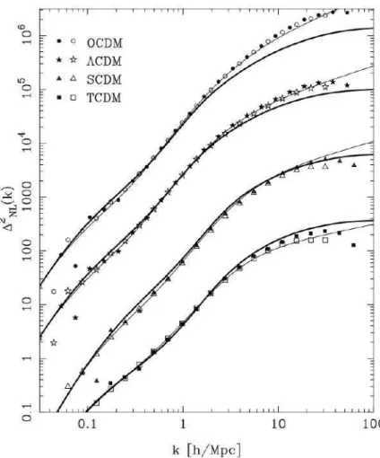
1.2.3 Non-linear regime . . . 37
Theoretical approach . . . 38
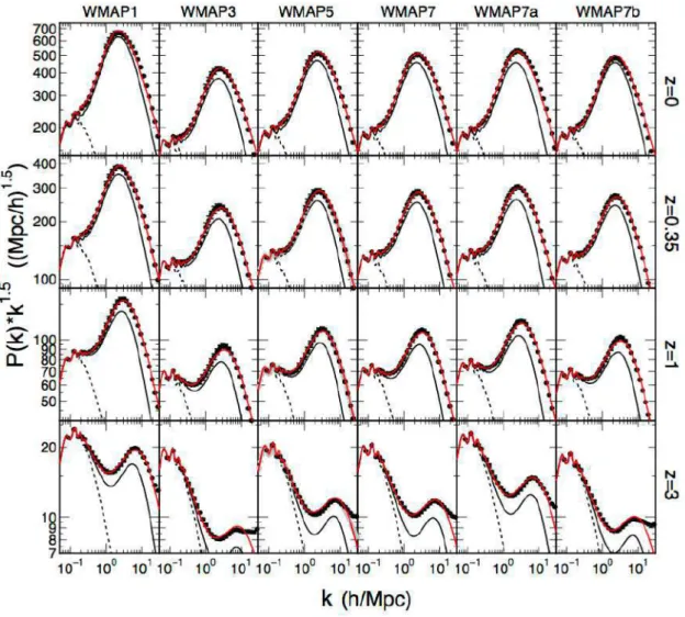
Halofit . . . 40
Halofit with Bird and Takahashi corrections . . . 42
HaloModel and emulators . . . 46
1.2.4 The galaxy bias . . . 47
Constant bias . . . 47
Linear redshift evolution . . . 48
Constant galaxy clustering . . . 48
Fry . . . 48
Merging model . . . 48
Tinker . . . 48
Croom . . . 49
Generalized time dependent bias . . . 50
1.3 Baryon acoustic oscillations and redshift-space distortions. . . . 50
1.3.1 BAO peak . . . 50
1.3.2 Redshift-space distortions . . . 52
1.3.3 Fingers-of-God . . . 53
1.3.4 Alcock-Pacyznski effect . . . 54
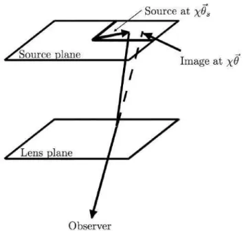
1.4 Weak gravitational lensing . . . 55
1.4.1 Regimes of gravitational lensing . . . 56
1.4.2 Geodesics and shear . . . 57
1.4.3 Ellipticity as an estimator of shear . . . 59
1.4.4 Weak lensing power spectrum . . . 60
1.5 Background cosmological probes . . . 61
1.5.1 Type Ia supernovae . . . 61
1.5.2 Cosmic microwave background . . . 65
1.5.3 The Hubble parameter . . . 68
1.5.4 The Hubble constant . . . 69
2 Cosmological parameter analysis 71 2.1 Basic concepts in probability and information . . . 72
Mathematical probability . . . 72
Frequentist probability . . . 72
Bayesian probability . . . 73
2.1.2 Bayes theorem . . . 73
2.1.3 Random variables . . . 74
Bayes theorem revisited . . . 75
2.1.4 The likelihood function . . . 75
2.2 Parameter and interval estimation . . . 76
2.2.1 Monte Carlo Markov chains . . . 76
Monte Carlo integration . . . 77
MCMC: basic concepts . . . 77 Metropolis-Hastings algorithm . . . 79 Other algorithms . . . 80 Chain convergence . . . 81 2.2.2 Profile-likelihood . . . 83 2.3 Goodness-of-fit . . . 84 2.4 Model comparison. . . 85
2.5 The Fisher matrix formalism . . . 87
2.5.1 Visualizing the confidence regions . . . 88
2.5.2 Limits of the formalism . . . 89
3 The Euclid mission 91 3.1 Spectroscopic and photometric redshift surveys . . . 92
3.1.1 Spectroscopic technique . . . 93
3.1.2 Photometric technique . . . 94
3.2 The Euclid satellite . . . 95
3.2.1 Primary and secondary science . . . 96
3.2.2 Satellite, service module and payload module . . . 98
3.2.3 VIS and NISP instruments . . . 99
3.2.4 Ground segment . . . 101
3.2.5 Surveys . . . 101
3.3 The Euclid Consortium . . . 102
3.4 The Inter-Science Taskforce for Forecasting . . . 104
4 Rh =ct and power law cosmologies confronted to CMB data 105 4.1 Context . . . 105
4.2 Models . . . 106
4.3 Method . . . 107
4.3.1 Goodness-of-fit and effect of correlations . . . 107
4.3.2 Model comparison . . . 110
4.4.1 Type Ia supernovae . . . 111
4.4.2 Baryon acoustic oscillations . . . 112
4.4.3 Cosmic microwave background . . . 113
4.5 Results . . . 123
4.6 Summary . . . 130
5 Cosmic acceleration and SNIa luminosity-redshift dependence133 5.1 Non-accelerated expansion at low-redshift . . . 134
5.1.1 Context . . . 134
5.1.2 Cosmological probes . . . 135
Type Ia supernovae . . . 135
Growth rate . . . 136
5.1.3 Goodness-of-fit and effect of correlations . . . 137
5.1.4 Results . . . 137
Background probes . . . 138
Background probes and growth rate of matter perturbations140 5.1.5 Summary . . . 144
5.2 Model-independent reconstruction of the expansion rate. . . 144
5.2.1 Context . . . 144
5.2.2 Cosmological probes . . . 145
Type Ia supernovae . . . 145
Baryon acoustic oscillations . . . 145
Cosmic microwave background . . . 147
5.2.3 Expansion rate reconstruction method . . . 147
5.2.4 Goodness-of-fit and effect of correlations . . . 150
5.2.5 Results . . . 151
Case 1: SNIa . . . 151
Case 2: SNIa+BAO. . . 153
Case 3: SNIa+BAO+CMB. . . 156
Growth rate . . . 160
The Hubble constant . . . 163
5.2.6 Summary . . . 163
6 Euclid forecasts: large-scale structure probe combination 167 6.1 Forecasting recipe . . . 169
6.1.1 General ingredients . . . 169
Cosmological context . . . 169
Fiducial cosmology and main survey specifications . . . . 171
Figure of Merit . . . 172
6.1.2 Spectroscopic galaxy clustering recipe . . . 173
Observable covariance matrix . . . 176
Fisher matrix . . . 176
6.1.3 Weak lensing recipe . . . 177
Observable . . . 177
Observable covariance matrix . . . 182
Fisher matrix . . . 183
6.1.4 Photometric galaxy clustering recipe . . . 183
6.1.5 Probe combination . . . 185
6.2 Forecasting in practice: the CosmoSIS code . . . 188
6.3 Weak lensing . . . 190
6.3.1 Baseline results . . . 191
6.3.2 Impact of intrinsic alignments . . . 195
6.3.3 Impact of massive neutrinos . . . 195
6.3.4 Non-linear correction and cut at non-linear scales . . . . 195
6.3.5 Non-flat universe . . . 196
6.3.6 Method and step of the numerical derivatives . . . 196
6.3.7 Boltzmann solver . . . 197
6.3.8 Summary . . . 198
6.4 Photometric galaxy clustering . . . 199
6.4.1 Baseline results . . . 199
6.4.2 Impact of galaxy bias . . . 203
6.4.3 Impact of massive neutrinos . . . 203
6.4.4 Non-linear correction and cut at non-linear scales . . . . 204
6.4.5 Non-flat universe . . . 204
6.4.6 Method and step of the numerical derivatives . . . 205
6.4.7 Boltzmann solver . . . 206
6.4.8 Summary . . . 206
6.5 Probe combination: photometric galaxy clustering and weak lens-ing . . . 208
6.5.1 Baseline results . . . 208
6.5.2 Impact of intrinsic alignments . . . 212
6.5.3 Impact of galaxy bias . . . 212
6.5.4 Impact of massive neutrinos . . . 213
6.5.5 Non-linear correction and cut at non-linear scales . . . . 213
6.5.6 Non-flat universe . . . 214
6.5.7 Method and step of the numerical derivatives . . . 214
6.5.8 Boltzmann solver . . . 215
6.5.9 Summary . . . 216
7 Generalized dark matter 225
7.1 Theoretical framework . . . 226
7.2 Current constraints . . . 228
7.2.1 Method . . . 229
7.2.2 Data sets . . . 232
7.2.3 Constraints from background cosmological probes . . . . 236
Constraints from CMB alone. . . 236
Constraints from all background probes . . . 236
7.2.4 Tension with H0 . . . 238
7.2.5 Non-linear regime . . . 239
7.2.6 Tension with weak lensing data . . . 241
7.2.7 Summary . . . 243
7.3 Euclid forecast . . . 247
7.3.1 Linear prediction . . . 247
7.3.2 Non-linear prediction . . . 248
7.3.3 Combination with real data . . . 250
7.3.4 Summary . . . 252
7.4 Degeneracy with dark energy . . . 253
7.4.1 Context . . . 253
7.4.2 Dark content(s) of the Universe . . . 254
Method and data samples . . . 254
Models . . . 255
Results . . . 258
7.4.3 Dark content(s) of the Universe: a Euclid forecast . . . . 261
Method . . . 261
Euclid spectroscopic survey . . . 264
Results . . . 264
7.4.4 Summary . . . 268
Conclusions 271 A Triangular plots of the Euclid forecasts 281 A.1 Additional ingredients to compute the forecasts . . . 281
A.2 Weak lensing . . . 288
A.3 Photometric galaxy clustering . . . 299
A.4 Probe combination: photometric Euclid survey . . . 311
A.5 CAMB and CLASS input files . . . 344
List of Figures 353
Bibliography 379
List of Abbreviations
ΛCDM Λ and Cold Dark Matter concordance model ΛGDM Λ and Generalized Dark Matter model
wCDM w (dark energy) and Cold Dark Matter model w0waCDM w0-wa (dark energy) and Cold Dark Matter model
2dFGRS 2-degree Field Galaxy Redshift Survey 2PCF 2-point-correlation function
6dFGS 6-degree Field Galaxy Survey AGN Active Galactic Nuclei
AIC Akaike Information Criterion
AICc Akaike Information Criterion - corrected AP Alcock-Pacyznski effect
BAO Baryon Acoustic Oscillations BBN Big Bang Nucleosynthesis BIC Bayesian Information Criterion
BOSS Baryon Oscillation Spectroscopic Survey CCDs Charge Coupled Devices
CDM Cold Dark Matter
CFHTLenS Canada France Hawaii Lensing Survey CMB Cosmic Microwave Background
COBE COsmic Background Explorer
CPL Chevallier-Polarski-Linder parametrization
CS Coasting Splines
DE Dark Energy
DES Dark Energy Survey
DESI Dark Energy Spectroscopic Instrument
eBOSS extended Baryon Oscillation Spectroscopic Survey
EC Euclid Consortium
ECB Euclid Consortium Board ECL Euclid Consortium Lead
eNLA extended Non-Linear Alignment model for IA ESA European Space Agency
FLRW Friedmann-Lemaître-Robertson-Walker metric
FoM Figure of Merit
GC Galaxy Clustering
GCp Galaxy Clustering - photometric GCs Galaxy Clustering - spectroscopic GDM Generalized Dark Matter
GTD Generalized Time Dependent galaxy bias model halofit halofit non-linear prescription
HaloModel Halo Model non-linear prescription HST Hubble Space Telescope
IA Intrinsic Alignment of galaxies
IST Inter-Science Taskforce for forecasting JLA Joint Light-curve Analysis
LRGs Luminous Red Galaxies
LSST Large Synoptic Survey Telescope MCMC Monte Carlo Markov Chain
NALPL Non-Accelerated Local Power Law
NASA National Aeronautics and Space Administration OUs Organizational Units
PLM PayLoad Module
PPF Parametrized Post-Friedmann framework QSO Quasi-Stellar Object
RPT Renormalized Perturbation Theory RSD Redshift-Space Distortions
SDCs Science Data Centers SDSS Sloan Digital Sky Survey SGS Science Ground Segment SNIa SuperNovae of type Ia
SNIa+ev SuperNovae of type Ia with luminosity evolution SOC Science Operation Center
SPT Standard Perturbation Theory
SVM SerVice Module
SWGs Science Working Groups
VIPERS VIMOS Public Extragalactic Redshift Survey
WL Weak Lensing
WMAP Wilkinson Microwave Anisotropy Probe XC Cross (X) - Correlations
List of Symbols
a scale factor
AIA IA multiplicative nuisance parameter
As amplitude of the initial matter power spectrum
b galaxy bias
c speed of light in vacuum ca adiabatic sound speed
CIA IA multiplicative nuisance parameter
Cijδgδg GCp tomographic angular spectra Cijδgγ XC tomographic angular spectra Cijγγ WL tomographic angular spectra cs rest-frame sound speed
cvis GDM viscosity parameter
D1 growth factor
dA angular diameter distance
dL luminosity distance
E dimensionless Hubble parameter
f growth rate
f σ8 weighted growth rate
fsky fraction of the sky observed G Newton’s gravitational constant h reduced Hubble constant
H Hubble parameter
H0 Hubble constant
k modulus of the wave mode in Fourier space k∥ k component along the line-of-sight
k⊥ k component perpendicular to the line-of-sight
m∗B SNIa observed peak magnitude in the rest-frame B band
MB1 SNIa absolute magnitude in the rest-frame B band nuisance parameter ne free electron number density
Neff effective number of relativistic degrees of freedom ni galaxy number density in the ith redshift bin
Nijδg GCp shot-noise Nijϵ WL shot-noise
ns slope of the initial matter power spectrum (spectral index)
Nur number of ultra-relativistic species
p pressure
Pdw de-wiggled power spectrum Pg galaxy power spectrum
Pm (& Pδδ) matter power spectrum
Pnw no-wiggles power spectrum
Ps GCs shot-noise
q0 deceleration parameter present value
R scaled distance to recombination rd BAO standard ruler
rs co-moving sound horizon
t cosmic time
T transfer function
TCMB temperature of the CMB w equation of state parameter Wδg
i GCp window function in the ith redshift bin
Wδg
i GCp window function in the ith redshift bin divided by χ
Wiγ shear window function in the ith redshift bin
Wiγ shear window function in the ith redshift bin including the IA
WiIA IA window function in the ith redshift bin Xe free electron fraction
z redshift
z∗ redshift of the last scattering epoch zd redshift of the baryon drag epoch α SNIa stretch nuisance parameter β SNIa color nuisance parameter βIA IA luminosity nuisance parameter
χ co-moving distance
∆M SNIa host galaxy nuisance parameter
∆mevo SNIa luminosity evolution nuisance term
δp pressure perturbation
ℓa angular scale of the sound horizon at recombination
ϵ ellipticity
ηIA IA redshift nuisance parameter
γ shear
κ convergence
Λ cosmological constant
µ distance modulus
Ωb baryon present energy density parameter
ωcdm cold dark matter reduced present energy density parameter Ωcdm cold dark matter present energy density parameter
ωdm dark matter reduced present energy density parameter Ωdm dark matter present energy density parameter
ΩK curvature present energy density parameter
ΩΛ Λ present energy density parameter
ωm matter reduced present energy density parameter
Ωm matter present energy density parameter
Ωr radiation present energy density parameter
ρ energy density
ρ0,crit critical present energy density
σ anisotropic stress
σ8 Root mean square mass fluctuations amplitude on 8 Mpc/h scales at z =0
σp GCs non-linear nuisance parameter
σv GCs non-linear nuisance parameter
Introduction
[Version française]
La cosmologie est la branche de la science qui étudie l’Univers, ou le cosmos, dans son ensemble. Son objectif principal est d’aborder des questions fonda-mentales pour la nature humaine, comme d’où venons-nous, où sommes-nous, où allons-nous et à quel rythme ? Fondamentalement, la cosmologie essaie de comprendre l’Univers dans lequel nous vivons en observant notre passé et finalement, de prédire notre avenir. Il y a un siècle, cela ressemblait à des ques-tions philosophiques et il semblait impossible d’y répondre par l’approche scien-tifique. Cependant, grâce à l’amélioration de nos connaissances théoriques et, dans les dernières décennies, l’amélioration de la technologie et des techniques d’observation, nous sommes maintenant en mesure de proposer des modèles théoriques pour expliquer notre Univers et, surtout, de les tester grâce aux observations. Ce fut le début de la cosmologie moderne. Une brève revue, fournissant les bases du cadre cosmologique, est présentée dans le chapitre1 de cette thèse.
Encore plus récemment, nous avons atteint une si bonne précision sur nos observations cosmologiques que nous pouvons dire que nous vivons dans l’ère de la cosmologie de précision. Nous avons ainsi clairement besoin d’outils statis-tiques robustes pour analyser les données. Nous présentons les bases des prin-cipaux outils utilisés dans ce travail dans le chapitre2. Il est intéressant de noter que nous disposons d’un modèle théorique très simple (avec seulement 7 paramètres), appelé ΛCDM, capable de reproduire presque toutes les obser-vations actuelles avec une grande précision. Cependant, ce modèle suppose l’existence d’un fluide sombre appelé matière noire froide et d’un second fluide sombre appelé énergie sombre sous la forme d’une constante cosmologique. Le premier est nécessaire pour expliquer le manque de matière suggéré par nos observations, tandis que le second est nécessaire pour expliquer la nature ac-célérée observée de l’expansion de l’Univers. Le problème est qu’il n’y a pas de détection directe de la matière noire froide, ou d’une constante cosmologique et, dans le cadre du modèle ΛCDM, ils ont une contribution d’environ 95 % de la densité totale d’énergie de l’Univers. Il est donc impératif d’essayer de com-prendre ces composantes sombres en proposant de nouveaux modèles théoriques et de les tester par rapport aux observations.
Depuis le début de la cosmologie moderne, de nombreux télescopes observent le ciel pour obtenir des mesures pour différentes sondes cosmologiques, comme les supernovae de type Ia, les oscillations acoustiques de baryons, le fond cos-mologique micro-onde, le groupement de galaxies ou les lentilles faibles. Il y a beaucoup de sondages en cours dont les données sont en train d’être analysées et qui semblent pointer vers des tensions dans le modèle standard ΛCDM qui pourraient éventuellement conduire à de la nouvelle physique. Il existe par ailleurs plusieurs projets qui verront le jour dans les années qui viennent avec le but de fournir d’excellentes observations et l’espoir d’illuminer le secteur som-bre de l’Univers. Les données de certains de ces sondages passés et actuels sont décrites dans le premier chapitre de cette thèse. Mais, ce travail est largement axé sur le futur satellite Euclid de l’Agence Spatiale Européenne, qui va sonder un énorme volume de la structure à grande échelle de l’Univers avec des groupe-ments de galaxies et des lentilles faibles. Par conséquent, nous présentons la mission de manière beaucoup plus détaillée dans le chapitre3 de la thèse.
L’objectif principal de cette thèse est de prédire le pouvoir contraignant d’Euclid pour le modèle de concordance ΛCDM et des extensions simples au-delà. Cependant, la principale différence par rapport à de nombreuses études dans la littérature est le traitement spécifique que nous utilisons pour la combi-naison des différentes sondes. Il est bien connu que la combicombi-naison de différentes sondes cosmologiques est un moyen très puissant de contraindre les modèles cosmologiques. La raison en est que les différentes sondes sont généralement sensibles à différents aspects dans la façon dont la gravité agit dans le cos-mos; par conséquent, les combiner peut casser certaines dégénérescences entre différents paramètres cosmologiques et améliorer sensiblement nos contraintes. Les sondes sont généralement combinées en supposant qu’elles sont statistique-ment indépendantes, ce qui peut être vrai dans certains cas, mais ce n’est cer-tainement pas le cas pour le regroupement de galaxies et les lentilles faibles si nous sondons le même volume de l’Univers. Dans ce travail, nous quantifions l’impact des corrélations croisées entre ces sondes pour le futur satellite Euclid et estimons l’amélioration de nos connaissances cosmologiques si nous prenons ces corrélations croisées en compte. Toute cette analyse est présentée dans le chapitre6 de la thèse.
Au-delà de la prédiction de la capacité contraignante d’Euclid pour ΛCDM (et certaines extensions), cette thèse aborde également les composantes sombres de l’Univers au-delà du modèle de concordance. Nous utilisons une approche phénoménologique pour décrire à la fois la matière noire et l’énergie sombre. En commençant par la matière noire, on suppose généralement qu’elle est sans collision et sans pression, même lorsque nous considérons des modèles au-delà de ΛCDM. Dans le chapitre7, nous considérons un modèle généralisé pour la
matière noire, où nous lui permettons d’avoir une certaine pression et une cer-taine vitesse du son, qui lissent essentiellement le groupement de galaxies à petite échelle. Nous présentons les contraintes obtenues avec les observations actuelles et nous prédisons également la capacité d’Euclid à contraindre la na-ture de cette matière noire.
Concernant l’énergie sombre, nous considérons un modèle phénoménologique exotique pour lequel le taux d’expansion de l’Univers est donné par une loi de puissance. Il y a eu quelques désaccords dans la communauté concernant ce modèle entre ceux qui prétendent qu’il peut reproduire les observations jusqu’au redshift z ∼ 2 et ceux qui prétendent le contraire. Dans ce travail, nous incluons, pour la première fois, des informations provenant du fond diffus cosmologique lors du test de ce modèle. C’est le sujet du chapitre4.
En dernier lieu, nous étudions la possible corrélation entre des systématiques astrophysiques dans les supernovae de type Ia et l’information cosmologique que nous en tirons. Plus en détail, nous étudions comment une dépendance de la luminosité intrinsèque des supernovae de type Ia avec le redshift peut influencer nos conclusions sur la nature accélérée de l’expansion de l’Univers. Cette étude est l’objet du chapitre5de cette thèse.
En résumé, l’objectif principal de cette thèse est de prédire la puissance con-traignante du futur satellite Euclid pour le modèle de concordance (et des exten-sions simples, chapitre6) et les modèles de matière noire exotique (chapitre7), avec une attention particulière portée sur l’impact des corrélations croisées quand on combine différentes sondes cosmologiques. En plus, nous analysons également un modèle d’énergie sombre exotique où le taux d’expansion de l’Univers est donné par une loi de puissance dans le chapitre4 et nous étu-dions l’impact d’une dépendance de luminosité intrinsèque des supernovae de type Ia avec le redshift sur les conclusions que nous pouvons tirer sur la nature accélérée de l’expansion cosmique dans le chapitre5.
Nous suivons la notation standard dans la littérature, sauf indication con-traire. Les indices latins correspondent aux trois coordonnées spatiales, tandis que les indices grecs correspondent aux quatre coordonnées d’espace-temps. Les indices répétés sont sommés. Les vecteurs sont indiqués par des lettres en carac-tères gras. Un point sur toute quantité désigne la dérivée temporelle de celle-ci. Un indice 0 indique le temps présent et nous utilisons des unités naturelles avec ¯h =c=1.
[English version]
Cosmology is the branch of science studying the Universe, or cosmos, as a whole. Its main goal is to address questions that are fundamental to human nature, like where do we come from, where are we, where are we going and at what pace. Basically, cosmology tries to understand the Universe we are living in by observing our past, and eventually predict our future. A century ago these interrogations looked like philosophical questions and it seemed im-possible to answer them with the scientific approach. However, thanks to the improvement on our theoretical knowledge and, especially in the last decades, the improvement of technology and observational techniques, we are now able to propose theoretical models trying to explain our Universe and, more impor-tantly, we can test them against the observations. This was the beginning of modern cosmology. A brief review of it, providing the basics of the cosmological framework, is presented in Chapter1 of this thesis.
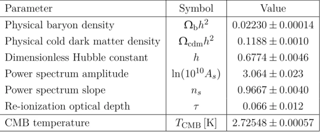
Even more recently, we have reached such a good precision on our cosmo-logical observations that we can say we live in the precision cosmology era. Therefore, we are in clear need of robust statistical tools to analyze the data. We present the basics of the main tools used in this work in Chapter2. Inter-estingly enough, we have a very simple (only 7 parameters) theoretical model, called ΛCDM, that is able to reproduce nearly all the current observations with great accuracy. However, this model assumes the existence of a dark fluid called cold dark matter and a second dark fluid called dark energy in the form of a cos-mological constant. The former is needed in order to explain the lack of matter in our observations, while the latter is required in order to explain the observed accelerated nature of the expansion of the Universe. The problem is that there is no direct detection of cold dark matter, or a cosmological constant, and in the ΛCDM framework they have a contribution of roughly 95 % of the total energy density of the Universe. It is therefore mandatory to try to understand these dark components by proposing new theoretical models and confront them with the observations.
Since the beginning of modern cosmology, there have been many telescopes observing the sky to obtain measurements for different cosmological probes, like type Ia supernovae, baryon acoustic oscillations, the cosmic microwave back-ground, galaxy clustering, or weak lensing. There are many ongoing surveys whose data is currently being analyzed, and which seem to point to some ten-sions within the standard ΛCDM model that could eventually lead to some new physics. And there are several projects that will occur in the future with the goal of providing exquisite observations, and the hope of shedding light on the dark sector of the Universe. Data from some of these past and current surveys is described in the first chapter of this thesis. But, this work is largely focused
on the future Euclid satellite from the European Space Agency, which is going to probe a huge volume of the large-scale structure of the Universe with galaxy clustering and weak lensing. We present this mission in much more detail in Chapter3 of the thesis.
The main goal of this thesis is to predict the constraining power of Euclid for the concordance ΛCDM model, and simple extensions beyond it. However, the key difference with respect to many studies in the literature is the spe-cial treatment we use for the combination of the different probes. It is well known that combining different cosmological probes is a very powerful way to constrain cosmological models. The reason being that different probes are usu-ally sensitive to different aspects of how gravity acts in the cosmos; therefore, combining them can break some degeneracies between different cosmological parameters and noticeably improve our constraints. Probes are usually com-bined assuming they are statistically independent, which might be true in some cases, but is definitely not true for galaxy clustering and weak lensing if we probe the same volume of the Universe. In this work we quantify the impact of the cross-correlations between these probes for the future Euclid satellite, and estimate the improvement on our cosmological knowledge if we take these cross-correlations into account. All this analysis is presented in Chapter6 of the thesis.
Beyond predicting the constraining ability of Euclid for ΛCDM (and simple extensions of it), this thesis also tackles the dark components of the Universe be-yond the concordance model. We use a phenomenological approach to describe both dark matter and dark energy. Starting with dark matter, it is usually assumed to be collision-less and pressure-less, even when we consider models beyond ΛCDM. In Chapter7we consider a generalized model for dark matter, where we allow it to have some pressure and some sound speed, which essen-tially smoothes out the clustering at small scales. We present the constraints obtained with state-of-the-art observations, and we also predict the ability of Euclid to constrain the nature of dark matter.
Concerning dark energy, we consider an exotic phenomenological model for which the expansion rate of the Universe is given by a power law. There has been some disagreement in the community concerning this model between those claiming that it can reproduce the observations up to redshift z ∼ 2, and those who claim the contrary. In this work we include, for the first time, information coming from the cosmic microwave background when testing this model. This is the subject of Chapter4.
As a last point, we study the possible correlation between type Ia super-novae astrophysical systematics and the cosmological information we derive from them. More in detail, we study how a redshift dependence of the type Ia
supernovae intrinsic luminosity may impact our conclusions about the acceler-ated nature of the expansion of the Universe. This is the subject of Chapter5 of this thesis.
Summarizing, the main goal of this thesis is to predict the constraining power for the future Euclid satellite for the concordance model (and simple extensions of it, Chapter6) and general dark matter models (Chapter7), paying special attention to the impact of cross-correlations when we combine different cosmological probes. In addition, we also analyze an exotic dark energy model where the expansion rate of the Universe is given by a power law in Chapter4, and we study the impact of type Ia supernovae intrinsic luminosity redshift dependence on the conclusions we can draw on the accelerated nature of cosmic expansion in Chapter5.
We follow the standard notation in the literature unless stated otherwise. Latin indices run over the three spatial coordinates, while greek indices run over the four spacetime coordinates. Repeated indices are summed. Vectors are indicated by letters in boldface. A dot over any quantity denotes the time-derivative of it. A subscript 0 denotes the present time, and we use natural units with ¯h=c=1.
Chapter 1
Cosmological framework
In this chapter we present a broad overview of the cosmological framework, with the goal of providing the main cosmological tools required to follow the rest of this thesis. More in particular, we divide this first chapter in four different sections. In Sec.1.1 we introduce the standard model in cosmology focusing on its background expansion. In Sec.1.2, Sec.1.3, and Sec.1.4 we describe the large-scale structure of the Universe commenting both on the formation of structures, and the distortion of light because of these structures. Finally, in Sec.1.5 we present the main cosmological probes used nowadays in cosmology to constrain our models.
1.1 Modern cosmology
Cosmology is the branch of physics that studies the Universe, or cosmos, as a whole. Its ultimate goal is to understand the origin, the evolution, and the structure of the Universe. In order to achieve this goal, cosmology needs to consider all the structures of the Universe on a huge range of scales; planets orbiting stars, stars forming galaxies, galaxies gravitationally bound into clus-ters, or even clusters within superclusters. Moreover, a lot of particle physics are required to properly understand the origins of our Universe. Because of it, and the difficulty of studying the Universe (theoretically or observationally), cosmology used to be close to philosophy. However, in the past decades we have started to be able to give quantitative answers to some of the most important questions concerning our Universe, like why is it so smooth? Or how did struc-tures form? We have been able to start providing these answers by combining our knowledge on fundamental physics and the precise astronomical observa-tions that we have nowadays. This shift from philosophy to science and our ability to propose theoretical models that can be tested quantitatively against observations has led us to the modern era of cosmology.
In the XIX century the Universe was considered a static system where bright objects where fixed in the sky, because of their lack of apparent motion. In 1915 Albert Einstein published his theory of General Relativity [Einstein,1915],
Figure 1.1: Original plot of Edwin Hubble from Hubble,1929, showing the velocity along the line-of-sight as a function of the distance for the observed galaxies. Notice the typographical er-ror in the velocity units being km/s.
describing gravity as the consequence of the curvature of spacetime generated by the distribution of mass and energy. A couple of years later, he applied his theory to cosmology for the first time [Einstein,1917] and, in order to get a static Universe from it, he was forced to introduce a constant in his equations: the cosmological constant Λ. However, in 1929 Edwin Hubble was able to measure the velocity along the line-of-sight for a few galaxies with known distances, and he found that most of these galaxies were actually moving away from us, the faster the further they were [Hubble, 1929] (see the original plot in Fig.1.1).
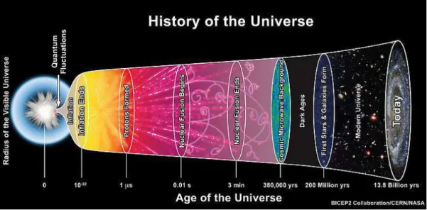
After realizing that the Universe was not static, but expanding, Einstein retracted from the introduction of the cosmological constant, and a new the-oretical model for the history of the Universe was developed: the Big Bang theory, where the Universe expands from an initial extremely high density and temperature state. This model is supported by astronomical observations, like the photons coming from the early Universe, or the abundance of primordial elements, and it is still one of the pillars of the standard model of cosmology.
Assuming the General Relativity theory of Einstein, the expansion of the Universe is only sensitive to the energy content, curvature, and pressure. Thus, for a Universe filled with matter (and radiation), there are only two final fates for the Universe: either the gravitational interaction is larger than the expansion originated from the Big Bang, leading to a Big Crunch where all the Universe comes back to a singularity, or it continues expanding forever but asymptotically converging to a static Universe (Big Chill). Surprisingly, in 1998 two different groups measured the distances to type Ia supernovae and found out that the
Figure 1.2: Intuitive interpretation of the scale factor. The co-moving distance between points on a hypothetical grid remains constant as the Universe expands, while the physical distance gets larger as time evolves.
Universe is not only expanding, but in an accelerated way [Riess et al., 1998; Perlmutter et al., 1999]. In the standard model of cosmology this acceleration is associated to an exotic fluid that only interacts through gravity and whose pressure is less than minus one third of its energy density. For the case where the pressure is exactly minus the energy density this fluid is equivalent to the cosmological constant first introduced by Einstein in 1917. More than 100 years later we have not been able to understand the nature of this constant (or fluid), if it is really there. This acceleration may also be due to a modification of the theory of gravity at cosmological scales, but, if we trust the theory of Einstein, current measurements tell us that the nature of about 95% of the energy content of the Universe remains still unknown.
1.1.1 A smooth and expanding universe
Scale factor and the FLRW metric
Thanks to the measurements performed since Hubble [Hubble, 1929], we have very good evidence to think that our Universe is expanding. This effect is commonly described by the so-called scale factor a, whose present value is set to one and was smaller in the past. In Fig.1.2 we can see an intuitive picture of the definition of the scale factor. Let us imagine the space as a grid expanding uniformly as a function of time. Two different points of this grid maintain their coordinates, so the co-moving distance (or difference between coordinates) remains constant. However, the physical distance is proportional to the scale factor, which evolves with time.
In addition to the scale factor, the Universe is usually also characterized by its geometry: flat, closed or open, that, according to General Relativity, is related to the energy content of the Universe.
Let us first consider the geometry of a three-dimensional homogeneous and isotropic space. Geometry is essentially encoded in the metric gij(x) (with the
indices i, j running over the three spatial coordinate labels), which gives the line element dl2 ≡ g
ijdxidxj (with summation over repeated indices). The
easiest metric for a homogeneous, isotropic, three-dimensional space is given by flat space, with line element dl2 = dx2. Another possibility is a spherical
(or hyper-spherical) surface in four-dimensional Euclidian (pseudo-Euclidian) space with some arbitrary positive constant radius a. The line elements are then given by
dl2 = dx2± dz2, z2± x2 =a2. (1.1)
Rescaling these coordinates by the constant a, the line elements in the spher-ical and hyper-spherspher-ical cases are
dl2 =a2!dx2± dz2", z2± x2 =1 . (1.2)
Computing the differential of the last equation we can write the line elements as dl2 =a2 # dx2±(x · dx) 2 1 ∓ x2 $ . (1.3)
We can then extend this to the Euclidian space by dl2 =a2#dx2+K(x · dx)2 1 − x2 $ , (1.4) where K ⎧ ⎪ ⎪ ⎨ ⎪ ⎪ ⎩ >0 spherical, <0 hyper-spherical, =0 Euclidian. (1.5) It can also be easily extended to the geometry of space-time by writing the line element as ds2 ≡ −gµνdxµdxν = dt2− a2(t) # dx2+K(x · dx) 2 1 − x2 $ , (1.6) where a(t) is now the scale factor of the Universe presented in Fig.1.2.
If the Universe appears spherically symmetric and isotropic to a set of freely falling observers, this is the unique metric of the Universe (up to a coordinate transformation). The components of this metric are then given by
gij =a2(t) ) δij +K x ixj 1 − Kx2 * , gi0 =0, g00 =−1 , (1.7) where x0 stands for the time coordinate, and the speed of light c has been set
to 1. Notice that another convention with an overall minus sign in the metric is also used in the literature.
In spherical polar coordinates we can write
dx2 = dr2+r2dΩ, dΩ ≡ dθ2+sin2θ dφ2, (1.8) giving ds2 =dt2− a2(t) # dr2 1 − Kr2 +r2dΩ $ . (1.9)
In this case the metric becomes diagonal,
grr = a 2(t)
1 − Kr2, gθθ =a2(t)r2, gφφ =a2(t)r2sin2θ, g00 =−1 . (1.10)
This is the so-called Friedmann-Lemaître-Robertson-Walker (FLRW) met-ric, and it is the standard one used in cosmology. It is important to notice that this metric is built on the cosmological principle, which states that the Universe is homogeneous and isotropic. Particularly, it states that the average properties of the Universe are the same in all locations and in all directions.
Dynamics of expansion
To understand the expansion of the Universe we need to determine the evolution of the scale factor, a, as a function of cosmic time, t. General Relativity tells us that this evolution is sensitive to the energy content of the Universe. In order to understand the dynamics of the expansion we need to apply the gravitational field equations of Einstein’s theory to the Universe. These equations can be written as
Rµν =−8πGSµν, (1.11)
where Rµν is the Ricci tensor,
Rµν = ∂Γλ λµ ∂xν − ∂Γλµν ∂xλ +Γ λ µσΓσνλ− ΓλµνΓσλσ, (1.12)
with Γµ
νκ being the affine connection,
Γµ νκ = 1 2gµλ # ∂gλν ∂xκ + ∂gλκ ∂xν − ∂gνκ ∂xλ $ , (1.13)
and Sµν can be expressed as a function of the energy-momentum tensor Tµν
Sµν ≡ Tµν−12gµνTλλ. (1.14)
If we take into account the standard FLRW metric, we can use several symmetries of it and simplify these equations. For instance, the components of the affine connection with two or three time indices all vanish, as well as the Ri0 =R0icomponents of the Ricci tensor. After some algebra we can write the
Ricci tensor as
R00 =3¨a
a, Rij =−
!
2K+2˙a2+a¨a"˜gij, (1.15)
where ˜gij is the three-dimensional metric.
In a homogeneous and isotropic universe the components of the energy-momentum tensor must take everywhere the form
T00 =ρ(t), T0i=0, Tij = ˜gij(x)a−2(t)p(t), (1.16)
where ρ(t) stands for the proper energy density and p(t) represents the proper
pressure. We can then write the tensor Sµν as
Sij =Tij− 12˜gija2 +
Tkk+T00,= 21(ρ− p)a2˜gij, (1.17)
S00 =T00+12+Tkk+T00,= 12(ρ+3p), (1.18)
Si0 =0 , (1.19)
and finally obtain the Einstein equations
−2Ka2 − 2˙a 2 a2 − ¨a a =−4πG(ρ− p), (1.20) 3¨a a =−4πG(3p+ρ). (1.21) Adding three times the first equation to the second we find the fundamental Friedmann-Lemaître equation [Friedmann, 1922; Friedmann, 1924; Lemaître,
1927], which provides the evolution of the expansion of the Universe as a func-tion of the energy content
˙a2+K = 8πGρa
2
3 . (1.22)
From the Einstein equations (Eq. (1.21) is also sometimes know as the ac-celeration equation) we can also extract the so-called conservation equation
˙ρ=−3˙a
a (ρ+p). (1.23)
Although Eqs. (1.21,1.22,1.23) are not independent because they all come from Einstein equations, all of them are very useful in cosmology. For instance, given p as a function of ρ we can solve Eq. (1.23) to get ρ as a function of a, and plug it into Eq. (1.22) to find a as a function of t.
Even without knowing the dependence of ρ as a function of a, we can define from Eq. (1.22) the critical present energy density
ρ0,crit≡ 3H 2 0
8πG. (1.24)
Independently of the contents of the Universe, the curvature constant K will be > 0, equal to 0, or < 0, if the present energy density ρ0 is greater, equal to,
or smaller than ρ0,crit.
Using Eq. (1.21) we can define the deceleration parameter today q0 as
q0≡ −¨a(t˙a02)(at(t0)
0) =
4πG 3H2
0(ρ0+3p0), (1.25)
where the subscript 0 denotes the present value, and t0is the age of the Universe
today.
Cosmic inventory
In order to fully understand the expansion of the Universe we need to know the evolution of ρ as a function of a. Although it is difficult to solve Eq. (1.23) in a general way, we can consider some frequently encountered extreme cases. Let us first assume that the pressure is related to the energy density through the equation of state parameter, w
p=wρ, (1.26)
and let us further assume w to be time-independent. Then Eq. (1.23) tells us that
ρ∝ a−3−3w. (1.27)
p=0 ⇒ ρ ∝ a−3. (1.28)
For radiation we get
p= 13ρ⇒ ρ ∝ a−4. (1.29)
And for a cosmological constant
p=−ρ ⇒ ρ =constant . (1.30)
With these relations between ρ and a, and assuming a flat Universe, we can use Eq. (1.22) to easily get the scale factor dependence on cosmic time. For instance, for a cold matter dominated universe a(t) ∝ t2/3, while a(t) ∝ t1/2 for a radiation dominated universe.
In general we do not have a single constituent of the Universe. For a mixture of cold matter, radiation, and a cosmological constant, the total energy density is given by ρ = 3H 2 0 8πG ! ΩΛ+Ωma−3+Ωra−4" , (1.31)
where ΩΛ, Ωm, Ωr stand for the present energy density parameter of the
cos-mological constant, cold matter, and radiation, respectively, which is defined as the ratio of the present energy density and the critical present energy density. We can then rewrite the Friedmann-Lemaître equation (1.22) for an arbitrary value of K as
H2(a) =H02!ΩΛ+Ωma−3+Ωra−4+ (1 − ΩΛ− Ωm− Ωr)a−2" , (1.32) where H(a) ≡ ˙a/a is the Hubble parameter, and the term (1 − ΩΛ− Ωm−
Ωr)a−2 can be associated to the curvature of the Universe
(1 − ΩΛ− Ωm− Ωr) = ΩK≡ − K
H02. (1.33)
1.1.2 Distances in the Universe
Measuring distances in the Universe is inherently tricky since, because of the expansion of the Universe, the distance to a given object varies with the prop-agation time of the emitted light. Looking back at Fig.1.2 we can immediately see two different definitions of distance: the co-moving distance, that remains fixed as the Universe expands; and the physical distance, which grows because of the expansion. In the following we will present different definitions for the
distance that will be useful depending on the observations that we have. All of them can be calculated from the fundamental distance measure: the distance on the co-moving grid.
Redshift
Since the speed of light is finite, when we measure the distance to a certain object we are looking at the past. Therefore, there is in intrinsic duality be-tween time and distance. It is characterized by a quantity called redshift. It is an observational phenomenon that indicates that the spectrum of a source is shifted towards red sequences because of the expansion of the Universe. It is a very interesting quantity from an observational point of view because it can be measured by atomic emission and absorption wavelengths. Notice that when objects have peculiar velocities their spectra can also be shifted (red if they are receding or blue if they are approaching us). This contribution to the redshift is then associated to the Doppler effect.
The redshift z can be related to the scale factor a. Let us consider a light ray emitted at time te with wavelength λe, and received at time tr with wavelength
λr. Since light travels in geodesics, ds2=0, using Eq. (1.9) we can write - tr te dt a(t) = - 0 R dr √1 −Kr2 = - tr+λr te+λe dt a(t), (1.34) which lead to - te+λe te dt a(t) = - tr+λr tr dt a(t). (1.35)
Assuming that the scale factor is constant over the small period of one cycle of a light wave we can write
1 ae(te+λe− te) = 1 ar(tr+λr− tr) ⇒ λr λe = ar ae , (1.36)
where ae =a(te) and equivalently for tr.
We can now define the redshift as
z ≡ λr− λe
λe . (1.37)
Taking ar =a0 =1 and ae just as an arbitrary a value, the redshift is then
given by
1+z = 1
Co-moving distance
The co-moving distance measures the distance between two objects in a coordi-nate system that expands with the Universe; thus, if these objects do not have peculiar velocities the distance between them will remain constant. We can define the co-moving distance between an object at scale factor a and us as
χ= - t0 t(a) dt′ a(t′) = - 1 a da′ a′2H(a′) = - z 0 dz′ H(z′). (1.39)
We can see objects typically with redshifts z ! 6. At these late times the radiation content can be ignored, so for a flat, matter-dominated Universe this integral can be solved analytically, giving
χ(a) = 2
H0 !
1 − a1/2" . (1.40)
Angular diameter distance
It is relatively easy in astronomy to measure the angle θ subtended by an object. We can measure the distance to an object by measuring this angle and knowing its physical size l. It will be given by (assuming θ is small)
dA = l
θ. (1.41)
In an expanding universe the moving size of the object is l/a. The co-moving distance to the object is given by Eq. (1.39), so the angle subtended will be given by θ = (l/a)/χ(a), giving the angular diameter distance
dA =aχ= 1χ
+z. (1.42)
This expression is only valid for a flat universe. It can be generalized to arbitrary non-vanishing values of ΩK with
dA = a H0.|ΩK| ⎧ ⎪ ⎨ ⎪ ⎩ sinh+√ΩKH0χ, ΩK>0 sin+√−ΩKH0χ, ΩK<0 . (1.43) Luminosity distance
Another way of measuring distances in cosmology is through the flux of an object with known luminosity. Let us first recall that the observed flux F at a distance d from a source of luminosity L is given by (in a static universe)
since the total luminosity through a spherical shell with area 4πd is constant. Let us now focus on the co-moving grid again and center the source at the origin. The observed flux will be given by
F = L(χ)
4πχ2(a), (1.45)
where L(χ)is the luminosity through a co-moving spherical shell of radius χ(a).
Let us also assume that all photons have been emitted with the same energy. The luminosity is then multiplied by the number of photons passing through a co-moving spherical shell per unit time. In a fixed time interval, photons travel farther on the co-moving grid at early times than at late times, since the associated physical distance at early times is smaller. Therefore, the number of photons crossing a shell in a fixed time interval will be smaller today than at emission by a factor a. In the same way, the energy of the photons will be smaller today than at emission. Thus, the energy per unit time passing through a co-moving shell a distance χ(a) from the source will be smaller than
the luminosity at the source by a factor a2. The observed flux will then be
F = La
2
4πχ2(a), (1.46)
where L is the luminosity at the source, and the luminosity distance will be given by
dL ≡ χ
a . (1.47)
1.1.3 Dark matter
The idea of having a non-baryonic contribution to matter in our Universe was first proposed in 1933 by Zwicky [Zwicky, 1933]. He measured the velocity dispersion of galaxies inside the Coma cluster, and he inferred from them a mass much smaller than the gravitational mass necessary for the galaxies random motion. Even by considering non-luminous baryonic matter to compensate for this deficit, it cannot be fully explained because the baryonic fraction is well constrained by baryon acoustic oscillations (see Sec.1.5).
Since Zwicky first proposal, there have been many observational evidence pointing towards the existence of a contribution to matter with a non-baryonic origin, from galactic to cosmological scales. In the following we will provide some examples at different scales, but a detailed compilation of dark matter evidence can be found in the review from Bertone, Hooper, and Silk,2005.
Figure 1.3: Original rotation curves of different galaxies (cir-cular velocity as a function of the distance to the galactic center) from Begeman, Broeils, and Sanders,1991. The dotted, dashed, and dash-dotted lines are the contributions of gas, disk, and dark matter, respectively.
Galactic scales
The most convincing evidence of dark matter on galactic scales comes from the analyses of the rotation curves of galaxies; i.e. the circular velocities of stars (and gas) as a function of their distance to the center of the galaxy. In Newtonian dynamics the circular velocity is given by
v(r) =
/
GM(r)
r , (1.48)
where M(r) ≡ 4π0 ρ(r)r2dr and ρ(r) the mass density profile. The velocity
should then be falling as 1/√r beyond the optical disk. However, it has been observed (see Fig.1.3 with the original rotation curves from Begeman, Broeils, and Sanders,1991) that v(r) is approximately constant, implying the existence
of a halo with M(r) ∝ r and ρ ∝ 1/r .
Other arguments for dark matter on sub-galactic and inter-galactic scales come from:
• Strong lensing around individual massive elliptical galaxies, which pro-vides evidence for substructure on scales of ∼ 106 solar masses [Metcalf
et al., 2004; Moustakas and Metcalf, 2003].
• Inconsistency between the amount of stars in the solar neighborhood and the gravitational potential implied by their distribution [Bahcall, Flynn, and Gould, 1992].
• Velocity dispersions of dwarf spheroidal galaxies, that imply mass-to-light ratios larger than those observed in our neighborhood [Mateo, 1998; Vogt et al., 1995].
• Velocity dispersions of spiral galaxy satellites, that suggest the existence of dark halos around spiral galaxies behind the optical disc [Azzaro, Prada, and Gutiérrez, 2004; Zaritsky et al., 1997].
Galaxy cluster scales
The mass of a cluster can be determined using different approaches, like ap-plying the virial theorem to the observed distribution of radial velocities, using weak lensing analyses, or studying the X-ray emission profile that traces the distribution of hot gas in rich clusters.
Let us consider the equation of hydrostatic equilibrium for a spherically symmetric system
1 ρ
dP
dr =−a(r), (1.49)
where P , ρ, and a are the pressure, density, and gravitational acceleration of the gas, respectively, at radius r. For an ideal gas it can be rewritten in terms of the temperature T . It can then be shown that for a baryonic mass of a typical cluster the temperature should obey the relation [Bertone, Hooper, and Silk,
2005] kT ≈(1.3 − 1.8)keV ) Mr 1014M ⊙ * ) 1 Mpc r * , (1.50)
where k is the Boltzmann’s constant, M⊙ is the solar mass, and Mr is the mass
enclosed within the radius r. The disparity between this temperature and the observed one (T ≈ 10 keV), suggests the existence of a substantial amount of dark matter in clusters.
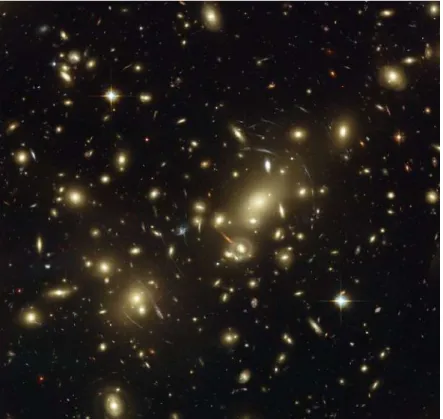
These conclusions have been checked using gravitational lensing data [Tyson, Kochanski, and Dell’Antonio, 1998]. According to General Relativity, photons propagate along geodesics that deviate from straight lines when passing near intense gravitational fields. Measuring the distortion of background objects due to the gravitational mass of a cluster enables us to determine its mass.
Cosmological scales
Many different cosmological probes are sensitive to the total quantity of bary-onic matter, or the total matter contribution to our Universe, like the photons coming from the early Universe (the cosmic microwave background), gravita-tional analyses at cosmological scales (weak lensing), the structure of visible matter in the Universe (baryon acoustic oscillations), or even type Ia super-novae analyses. All these probes will be presented in detail in Sec.1.5. We just focus here on one of the fundamental cosmological observations known as the Big Bang nucleosynthesis (BBN).
Since the Universe is expanding, its temperature was higher in the past. Just extrapolating, we can imagine a moment when the temperature was high enough for nuclear reactions to take place, as it is the case in the core of the stars. These nuclear reactions allow for the formation of light elements, like Helium or Lithium, from the combination of protons and neutrons. We refer to this process as BBN. Knowing the conditions of the early Universe and the relevant nuclear cross-sections, we can predict the expected primordial abundances of these light elements. In Fig.1.4 we show the predictions of BBN for these abundances and the agreement with the observations.
Interestingly enough, the BBN predictions for the abundances depend on the density of protons and neutrons at that time. The combined proton plus neutron density is the baryon density, so BBN gives us a way to measure the baryon density in the Universe. Since we know how those densities scale as a function of the scale factor, we can turn the measurements of light element abundances into measures of the baryon density today. BBN measurements tell us that nowadays baryonic matter contributes only around 5% to the critical density of the Universe. Since the total matter density today is certainly larger than this, BBN provides an extra evidence for the existence of dark matter.
1.1.4 Cosmic acceleration: a cosmological constant and
dark energy
Measuring distances at redshifts z > 0.1 are cosmologically interesting because these redshifts are large enough to have a small contribution from peculiar motions of the sources, and they are also large enough to be forced to take
Figure 1.4: Original plot from the Particle Data Group 2016 (and 2017 update) Review [Patrignani et al., 2016]. The BBN predictions for the primordial abundances of 4He, D, 3He, and 7Li are shown (as bands) as a function of the baryon-to-photon
ratio. The corresponding observations are represented by yellow boxes. The vertical narrow band corresponds to the cosmic mi-crowave background measurement of the baryon-to-photon ratio, while the wider vertical band represents the constraints from the combination of the different abundance measurements.
into account the effects of the cosmological expansion when determining the distances. In order to measure these distances we look for “standard candles” in the sky. These are objects with known absolute luminosity, so we can extract the luminosity distance by measuring their flux. For many years, the standard candles used were the brightest galaxies in rich galaxy clusters, but it is now well known that their absolute luminosity evolves significantly over cosmological time scales.
Fortunately, type Ia supernovae (SNIa) are nice candidates to replace these bright galaxies. SNIa are very bright objects easy to spot even at high redshifts, and, although they are not directly standard candles, they can be standardized by correcting for empirical effects (see Sec.1.5.1 for a more detailed discussion
![Figure 1.4: Original plot from the Particle Data Group 2016 (and 2017 update) Review [Patrignani et al., 2016 ]](https://thumb-eu.123doks.com/thumbv2/123doknet/2141050.8863/49.892.218.646.131.611/figure-original-particle-data-group-update-review-patrignani.webp)