Real-Time Fixed and Dynamic Priority Driven Scheduling Algorithms: Theory and Experience

HAL Id: inria-00073611

https://hal.inria.fr/inria-00073611

Submitted on 24 May 2006

HAL is a multi-disciplinary open access archive for the deposit and dissemination of sci-entific research documents, whether they are pub-lished or not. The documents may come from teaching and research institutions in France or abroad, or from public or private research centers.

L’archive ouverte pluridisciplinaire HAL, est destinée au dépôt et à la diffusion de documents scientifiques de niveau recherche, publiés ou non, émanant des établissements d’enseignement et de recherche français ou étrangers, des laboratoires publics ou privés.

Scheduling Algorithms: Theory and Experience

Jean-François Hermant, Laurent Leboucher, Nicolas Rivierre

To cite this version:

Jean-François Hermant, Laurent Leboucher, Nicolas Rivierre. Real-Time Fixed and Dynamic Priority Driven Scheduling Algorithms: Theory and Experience. [Research Report] RR-3081, INRIA. 1996. �inria-00073611�

ISSN 0249-6399

a p p o r t

d e r e c h e r c h e

Real-time fixed and dynamic priority driven

scheduling algorithms: theory and experience

Jean-François HERMANT, Laurent LEBOUCHER, Nicolas RIVIERRE

N˚ 3081

Décembre 1996

THEME 1

Unité de recherche INRIA Rocquencourt

Domaine de Voluceau - Rocquencourt - B.P. 105 - 78153 LE CHESNAY Cedex (France) Téléphone : +33 1 39 63 55 11 - Télécopie : +33 1 39 63 53 30

Jean-François HERMANT

1

, Laurent LEBOUCHER

2

,

Nicolas RIVIERRE

1

Thème 1 : Réseaux et systèmes

Projet REFLECS

Rapport de recherche n˚3081 - Décembre 1996

139 pages

Abstract: There are two main positions regarding real-time scheduling algorithms. The first is based on fixed priorities and the second makes use of dynamic priorities such as dead-lines. These two approaches have never really been compared because the emphasis has always been on the ease of implementation rather than the efficiency of the algorithms and the complexity of the associated feasibility conditions. In addition to traditional real-time applications, we believe that starting to look at these two criteria will be very important from the point of view of providing admission control mechanisms and real-time guarantees on large distributed systems like the Internet network.

To that end, our purpose is first to provide a general framework based, on the one hand, a representation of preemptive, real-time scheduling in an algebraic structure that enables us to evaluate the distance of the optimality of any scheduling algorithm ; and on the other hand, a consistent representation of the associated feasibility conditions that enables us to evaluate the number of basic operations. As a second step, considering several kinds of traf-fics, we initiate the comparison by a straight, but limited, application of our general frame-work. Our preliminary results will notably highlight, in the cases where deadlines are all greater than periods, that fixed priority schedulers (like deadline monotonic) behave as well as EDF while the worst-case response time analysis is less complex. The same observation is valid when the task sets are almost homogeneous but is in favor of EDF in the general case or when a simple feasibility analysis is needed.

Therefore, it might be of interest, given a real-time scheduling context (spanning from small embedded systems to large distributed systems), to take into account these two extra criteria in order to find a right trade-off among several possible solutions.

Key-words:busy period, comparison, complexity, efficiency, dynamic priority, fixed prior-ity, preemptive, real-time, scheduling.

1. INRIA, Projet REFLECS, B.P. 105, 78153 LE CHESNAY Cedex (France) Email: {Jean-Francois.Hermant, Nicolas.Rivierre}@inria.fr

2. CNET, France Télécom, PAA/TSA/TLR,

38-40, rue du Général Leclerc, 92794 ISSY-LES-MOULINEAUX Cedex 9 (France) Email: lebouche@issy.cnet.fr

Résumé :Il existe deux principales familles d’algorithmes d’ordonnancement temps réel, la première s’appuyant sur des priorités fixes et la seconde sur des priorités dynamiques de type échéances. Celles ci n’ont jamais été vraiment comparées l’une à l’autre, si ce n’est en termes de mise en oeuvre. Notre propos est d’initier une telle comparaison en termes d’effi-cacité des algorithmes ainsi que de complexité des conditions de faisabilité associées. Au delà des applications temps réel traditionnelles, commencer à considérer ces deux critères nous semble devenir critique dans la perspective de la fourniture de mécanismes de contrôles d’admission et de garanties temps réel sur de grands systèmes répartis tels qu’Internet. Dans un premier temps, nous introduisons un cadre général basé, d’une part, sur une repré-sentation de l’ordonnancement temps réel préemptif sous forme de structure algébrique per-mettant d’évaluer la distance à l’optimalité de tout algorithme et, d’autre part, sur une représentation homogène des conditions de faisabilité associées permettant d’évaluer le nombre d’opérations élémentaires induites. Dans un deuxième temps, considérant différents types de trafics, nous initialisons la comparaison par une application directe, mais limitée, de notre cadre général. Nos résultats préliminaires font notamment apparaître, lorsque les échéances des tâches sont toutes supérieures aux périodes que les algorithmiques d’ordon-nancement à priorité fixes (comme Deadline Monotonic) se comportent aussi bien qu’EDF alors que l’analyse des pires temps de réponses des tâches est moins complexe. La même remarque s’applique en présence de tâches homogènes mais reste en faveur de EDF dans le cas le plus général ou lorsqu’une simple analyse de faisabilité est nécessaire.

Il semble donc être intéressant, en fonction du contexte d’ordonnancement (allant du petit système embarqué jusqu’au grand système distribué) de faire intervenir les critères d’effica-cité et de complexité pour choisir l’algorithme temps réel le plus adapté.

Mots-clé : comparaison, complexité, efficacité, période occupée, priorité fixe, priorité dynamique, ordonnancement, préemptif, temps réel.

Contents

Glossary

6

1

Introduction

8

1.1

Model, concepts and notations

8

1.1.1

Model

8

1.1.2

Classic concepts

10

1.2

Previous work

11

1.2.1

Dynamic priority driven scheduling algorithms

12

1.2.1.1

Optimality

12

1.2.1.2

Feasibility

12

1.2.1.3

Worst-case response time

15

1.2.1.4

Shared resources and release jitters

17

1.2.2

Fixed priority driven scheduling algorithms

18

1.2.2.1

Optimality

18

1.2.2.2

Feasibility condition and worst-case response time

18

1.2.2.3

Shared resources and release jitter

21

1.3

Goals

21

2

Framework

24

2.1

Efficiency Framework

24

2.1.1

Scheduling referential

24

2.1.2

Periodic scheduling referential, algebraic structure and valid norms

25

2.1.3

Efficiency and finest criterion

28

2.1.4

Σ

-regions of Fixed-Priority based scheduling referentials

31

2.1.5

Efficiency computation procedure

32

2.1.5.1

Preliminary results

33

2.1.5.2

Efficiency procedure

35

2.2

Complexity framework

40

2.2.1

The necessary and sufficient feasibility tests

41

2.2.1.1

The feasibility tests in a «

» form

41

2.2.1.2

The feasibility tests in a «

» form

41

2.2.2

From intractable to tractable feasibility tests

42

2.2.2.1

The feasibility test for EDF in a «

» form

43

2.2.2.2

The feasibility tests in a «

» form

44

2.2.3

Improvements of the feasibility tests

49

2.2.4

The feasibility tests in their optimized form

49

2.2.4.1

The optimized feasibility test for EDF in a «

» form

49

2.2.4.2

The optimized feasibility tests in a «

» form

52

t

∈

S

∀

,

P t

( )

i

∀

∈

[

1 n

,

]

,

r

_i

≤

D

_i

t

∈

S

∀

,

P t

( )

i

∀

∈

[

1 n

,

]

,

r

_i

≤

D

_i

t

∈

S

∀

,

P t

( )

i

∀

∈

[

1 n

,

]

,

r

_i

≤

D

_i

2.2.5

Complexity comparison of the optimized feasibility tests

58

2.2.6

Summary

59

3

Efficiency of fixed and dynamic priority driven scheduling algorithms

60

3.1

Upper bound on the N

_U

-efficiency of EDF

60

3.2

Lower bound on the efficiency of any fixed priority scheduling algorithm

61

3.2.1

Preliminary results

61

3.2.2

Efficiency theorem

62

3.3

Applications of the efficiency theorem

63

3.4

A general method to compare the efficiency of scheduling algorithms.

66

4

Complexity of fixed and dynamic priority driven scheduling algorithms

68

4.1

Complexity analysis

70

4.1.1

The optimized feasibility test for EDF in a «

» form

70

4.1.2

The optimized feasibility tests in a «

» form

72

4.1.2.1

Fixed Priority based scheduling algorithms

72

4.1.2.2

The Earliest Deadline First scheduling algorithm

76

4.2

Complexity comparison

81

4.2.1

The optimized feasibility test for EDF in a «

» form

81

4.2.1.1

Upper bound on the cost of the optimized feasibility test

81

4.2.1.2

Lower bound on the cost of the optimized feasibility test

81

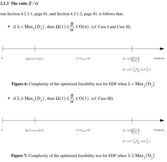
4.2.1.3

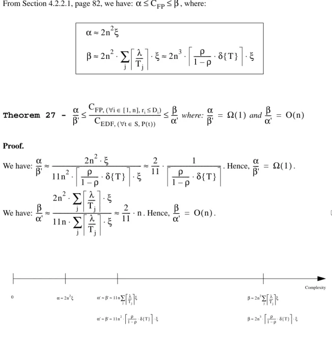
The ratio

82

4.2.2

The optimized feasibility tests in a «

» form

82

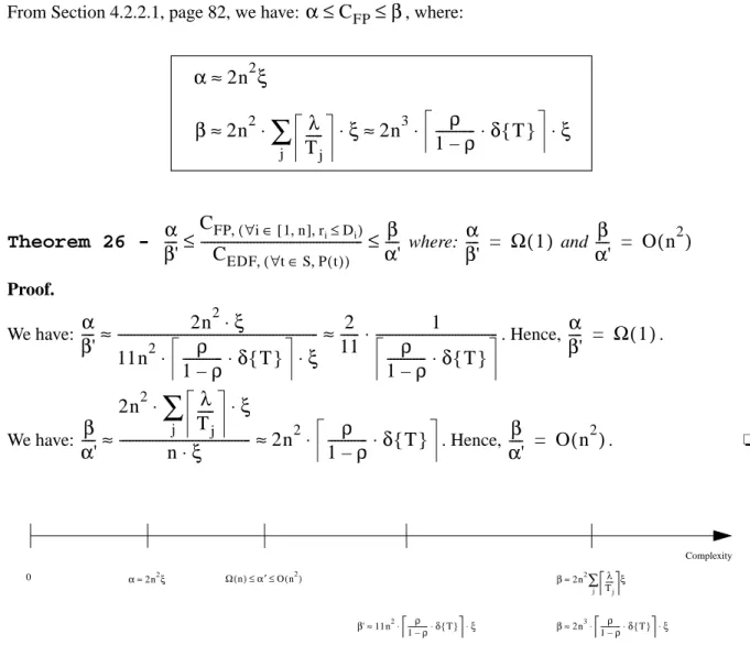
4.2.2.1

Fixed Priority based scheduling algorithms

82

4.2.2.2

The Earliest Deadline First scheduling algorithm

84

4.2.3

Complexity Theorems

88

4.2.3.1

The ratio

88

4.2.3.2

The ratio

90

4.2.4

Summary

91

4.3

Application of the complexity theorems

92

4.3.1

Homogeneous traffics

92

4.3.1.1

The feasibility test for EDF in a «

» form

92

4.3.1.2

The feasibility tests in a «

» form

93

4.3.1.3

Summary

95

4.3.2

Heterogeneous traffics

96

4.3.2.1

The feasibility test for EDF in a «

» form

96

4.3.2.2

The feasibility tests in a «

» form

98

5

Numerical examples

101

5.1

Particular scheduling referential

101

5.2

Efficiency performances

105

5.3

Computational Complexity

111

t

∈

S

∀

,

P t

( )

i

∀

∈

[

1 n

,

]

,

r

_i

≤

D

_i

t

∈

S

∀

,

P t

( )

β

'

⁄

α

'

i

∀

∈

[

1 n

,

]

,

r

_i

≤

D

_i

C

_{FP ∀i∈[1 n, ] r} i≤Di , ( ) ,

⁄

C

EDF,(∀t∈S P t, ( ))

C

_{EDF ∀i∈[1 n, ] r} i≤Di , ( ) ,

⁄

C

FP,(∀i∈[1 n, ],r_i≤D_i)

t

∈

S

∀

,

P t

( )

i

∀

∈

[

1 n

,

]

,

r

_i

≤

D

_i

t

∈

S

∀

,

P t

( )

i

∀

∈

[

1 n

,

]

,

r

_i

≤

D

_i

6

Synthesis

116

7

Conclusion

119

Appendix A

120

A.1

The sequence

is increasing, bounded, therefore convergent.

120

A.2

The limit

is bounded by

. 121

A.3

How much worth is it to solve

by successive iterations?

122

Appendix B

127

B.1

The sequence

,

.

How to obtain a faster convergence?

128

B.2

The sequence

,

.

How to obtain a faster convergence?

129

Appendix C

131

C.1

Task parameters

131

C.2

Computational Complexity -- Highest Priority First / Deadline Monotonic

133

C.3

Computational Complexity -- Earliest Deadline First

135

References

138

λ

_i( )k

{

}

_k≥0

λ

_i

λ

_i( )k k→+∞

lim

=

Min

ρ

_i

⋅

LCM

_l≤i

{ }

T

_l

1

1

–

ρ

_i

---

C

_j j

∑

≤i

⋅

,













λ

_i

=

W

_i

( )

λ

_i

w

_{i q}( )_,k

{

}

_k≥0

w

_{i q}( )_,0

=

0

L

_i( )k

( )

a

_l

{

}

_k≥0

L

_i( )0

( )

a

_l

=

0

Glossary

Worst-case computation time for task (cf. Section 1.1.1, page 8). Relative deadline for task (cf. Section 1.1.1, page 8).

Earliest Deadline First scheduling algorithm (cf. Section 1.2.1.1, page 12). Highest Priority First / Deadline Monotonic scheduling algorithm (cf. Section 1.2.2.1, page 18).

Highest Priority First / Rate Monotonic scheduling algorithm (cf. Section 1.2.2.1, page 18).

Processor demand function (cf. Section 1.1.2, page 10). Length of a deadline-( ) busy period.

Necessary and Sufficient Condition. EDF valid norm (cf. Theorem 13, page 26).

Processor utilization valid norm (cf. Theorem 13, page 26). Base period (cf. Section 1.1.2, page 10).

Periodic Non-Concrete Task set (cf. Definition 8, page 25). Class of PNTS (cf. Definition 8, page 25).

Worst-case response time for task (cf. Section 1.1.2, page 10). Period for task (cf. Section 1.1.1, page 8).

Processor utilization (cf. Section 1.1.1, page 8) later called N_U.

Length of the level-i busy period starting qT_i before the current activation of task (cf. Section 1.2.2.2, page 18).

Cumulative workload function (cf. Section 1.1.1, page 8).

f-efficiency of a scheduling algorithm P with respect to Σ (cf. Definition 12, page 28).

Efficiency of a scheduling algorithm P with respect to Σ (cf. Definition 12, page 28).

Length of the synchronous processor busy period (cf. Section 1.1.2, page 10). Length of a level-i busy period (cf. Section 1.1.2, page 10).

Class of scheduling algorithms (cf. Definition 3, page 24). Scheduling referential (cf. Definition 3, page 24).

Class of task sets (cf. Definition 3, page 24). Non-concrete task set (cf. Section 1.1.1, page 8). Non-concrete task of (cf. Section 1.1.1, page 8).

Σ-region of a scheduling referential (cf. Section 1.1.1, page 8).

C

_i

τ

_i

D

_i

τ

_i

EDF

HPF/DM

HPF/RM

h t

( )

L

_i

( )

a

a

+

D

_i

NSC

N

_EDF

N

_U

P

PNTS

τ

PNTSC

r

_i

τ

_i

T

_i

τ

_i

U

w

_{i q,}

τ

_i

W t

( )

α

_f

( )

P

ε

( )

P

λ

λ

_i

Π

Σ

=

( , )

ϒ Π

ϒ

τ

τ

τ

τ

_i

τ

_i

τ

χ Σ

( )

C

₁

⋅

e

_{7 5,}

+

C

₂

⋅

e

_{11 7,}

+

C

₃

⋅

e

_{13 10,}

Σ

–

region EDF

Σ

–

region HPF/DM

1 Introduction

Scheduling theory as it applies to hard real-time environment has been widely studied in the last twenty years. The community of real-time researchers is currently split into two camps, those who support fixed priority driven scheduling algorithms, that were devised for easy implementation, and those who support dynamic priority driven scheduling algorithms that were considered better theoretically. More-over since [LL73], a milestone in the field of hard real-time scheduling, these two classes of algorithms have been studied separately and a lot of results such as optimality, feasibility condition, response time, admission control have been established, relaxing some initial assumptions and considering several scheduling contexts. Consequently, these results are quite dispersed in the literature and the proofs have often been established in an ad-hoc manner.

In our opinion, the implementation and the hardware of today no longer justify a simple refusal of dynamic priority algorithms. On the other hand, the theoretical dominance of dynamic priority driven scheduling algorithms is not a determining factor in every context. Moreover, the concepts used by all the existing results are quite similar. Therefore, it is the first goal of this paper to build a consistent the-oretical framework which could encompass the collection of existing results and that enables us to evaluate the preemptive, non-idling fixed/dynamic priority driven scheduling algorithms in terms of

efficiency (the distance of the optimality) and the associated feasibility conditions in terms of complex-ity (the number of basic operations). As a second step, this paper will initiate such a comparison by a

straight, but limited, application of our framework considering several kinds of traffics.

More precisely, the paper is organized as follows. Section 1, page 8, outlines the computational model, recalls the basic scheduling concepts and proposes a state-of-the-art regarding preemptive, fixed/ dynamic priority driven scheduling algorithms. The goals of this paper are detailed at the end of this section.

Section 2, page 24, presents our framework to compare scheduling algorithms. To that end, we first propose an algebraic structure for preemptive, real-time scheduling that enables us to evaluate the gap separating a particular scheduling algorithm from an optimal one. Secondly a consistent representation of the feasibility conditions is proposed that enables us to compare the number of basic operations involved by these conditions.

Section 3, page 60 (resp. Section 4, page 68), proposes a straight, but limited (in the sense that many refinements or other results might be derived from Section 2, page 24), application of our abstract framework to initiate the efficiency comparison (resp. complexity comparison) of fixed versus dynamic priority driven scheduling algorithms in presence of general task sets, as well as particular task sets. The obtained preliminary results are illustrated in Section 5, page 101, with some simple but represen-tative numerical examples (e.g. voice and image traffics versus embedded system traffics).

Finally, Section 6, page 116, is a synthesis of our fixed/dynamic priority driven scheduling algorithm comparison leading to new arguments in that controversial discussion.

1.1 Model, concepts and notations

1.1.1 Model

In this paper, we shall consider the problem of scheduling a set of n non-concrete periodic or sporadic tasks on a single processor. This will be done in presence of hard real-time con-straints and with relative deadlines not necessarily related to the respective periods of the tasks. A task is a sequential job that is invoked with some maximum frequency and result in a single execution of the job at a time, handled by a given scheduling algorithm. From the scheduling point of view, a task can then be seen as an infinite number of activations. By definition, we consider that:

•

A non-concrete periodic task recurs and is represented by the t-uple , where , and respectively represent its worst-case computation time, relative deadline and

τ

=

{

τ

₁

, ,

… τ

_n

}

τ

_i

τ

_i (

C

_i

, ,

D

_i

T

_i)

period (note that the absolute deadline of a given activation is equal to the release time plus the relative deadline). A concrete periodic task is defined by where , the start time, is defined as the duration between time zero and the first activation of the task.

•

A non-concrete periodic task set is a set of n non-concrete tasks. A

con-crete periodic task set is a set of n concrete tasks. Therefore, an infinite number of concrete task sets can be generated from a non-concrete task set (without loss of

generality we assume ).

Note that a concrete periodic task set is called a synchronous task set iff for all ( is then called a critical instant in the literature) otherwise, is called an

asynchronous task set ([LM80] showed that the problem to know if an asynchronous task set

can lead to a critical instant is NP-complete).

•

Sporadic tasks were formally introduced in [MOK83] (although already used in some papers,

e.g., [KN80]) and differ only from periodic tasks in the activation time: the (k+1)th activation of a periodic task occurs at time , while it occurs at if the task is sporadic. Hence represents the minimum interarrival time between two successive acti-vations.

•

A general task set is a non-concrete periodic or sporadic task set such that , and are not related. On the other hand, a particular task set is a non-concrete task set such that , and are related.

Throughout this paper, we assume the following:

•

all the studied schedulers make use of the HPF (Highest Priority First) on-line algorithm but differ by their priority assignment scheme (in the sequel, we will no more refer to HPF). They all make use of a fixed tie breaking rule between tasks that show the same priority. They are

non idling (i.e., the processor cannot be inactive in presence of pending activations) and preemptive (i.e., the processing of any task can be interrupted by a higher priority task).

•

, , and general, as well as particular, task sets will be considered.

More precisely, the following task sets will be considered:

-

general case, , and are not related,

-

homogeneous case, , and ,

-

, ,

-

, ,

-

(all the deadlines are supposed to be dominated by all the periods),

-

, ,

-

(all the periods are supposed to be dominated by all the deadlines).

•

all tasks in the system are independent of one another and are critical (hard real-time), i.e., all of them have to meet their absolute deadline. Unless otherwise stated, tasks do not have resour-ce constraints and the overhead due to context switching, scheduling... is considered to be in-cluded in the execution time of the tasks.

•

time is discrete (tasks activations occur and task executions begin and terminate at clock ticks; the parameters used are expressed as a multiples of clock ticks); In [BHR90], it is shown that there is no loss of generality with respect to feasibility results by restricting the schedules to be discrete, once the task parameters are assumed to be integers.

ω

_i

{

τ

_i

,

s

_i

}

s

_i

τ

=

{

τ

₁

, ,

… τ

_n

}

ω

=

{

ω

₁

,

… ω

,

_n

}

min

_{1≤ ≤i n}

{ }

s

_i

=

0

ω

s

_i

=

s

_j

1

≤

i j

,

≤

n

s

_i

ω

t

_k+1

=

t

_k

+

T

_i

t

_k+1

≥

t

_k

+

T

_i

T

_i

τ

=

{

τ

₁

, ,

… τ

_n

}

i

∀

∈

[

1 n

,

]

T

_i

D

_i

τ

=

{

τ

₁

, ,

… τ

_n

}

∀

i

∈

[

1 n

,

]

T

_i

D

_i

i

∀

∈

[

1 n

,

]

C

_i

≤

T

_i

C

_i

≤

D

_i

i

∀

∈

[

1 n

,

]

T

_i

D

_i

i

∀

∈

[

1 n

,

]

T

_i

=

T

D

_i

=

D

i

∈

[

1 n

,

]

∀

D

_i

=

T

_i

i

∈

[

1 n

,

]

∀

D

_i

≤

T

_i

D

_i

{ }

«

{ }

T

_i

i

∈

[

1 n

,

]

∀

D

_i

≥

T

_i

D

_i

{ }

»

{ }

T

_i

1.1.2 Classic concepts

Let us now recall some classic concepts used in hard real-time scheduling:

•

the scheduling of a concrete task setω is said to be valid if and only if no task activation misses its absolute deadline.

•

a concrete task setω is said to be feasible with respect to a given class of scheduling algorithms if and only if there is at least one valid schedule that can be obtained by a scheduling algorithm of this class (in this paper, we consider only two classes of scheduling algorithms combining non-idling, preemptive, fixed/dynamic priority driven scheduling algorithms). Similarly, a non-concrete task setτ is said to be feasible with respect to a given class of scheduling algo-rithms if and only if every concrete task setω that can be generated fromτ is feasible in this class.

Note that from the real-time specification point of view, a non-concrete task set is more realis-tic than a concrete one, since not one but all the patterns of arrival are indeed considered. For the same reasons, but from the scheduling point of view, a feasibility condition for a non-con-crete task set is generally more selective and less complex than one for a connon-con-crete task set. In particular [BHR90], [BMR90] showed that a concrete task set cannot, in general, be tested in a polynomial time unless P=NP. Anyhow, they also showed that a concrete synchronous task set, or a non-concrete task set, can be tested in pseudo polynomial time whenever the processor utilization (i.e. with a constant smaller than 1).

•

a scheduling algorithm is said to be optimal with respect to a given class of scheduling algo-rithms if and only if it generates a valid schedule for any feasible task set in this class. Note that this definition is ambiguous since it is class of scheduling algorithm dependent. In Section 2.1, page 24, we will precise this concept with respect to a given scheduling referential.

•

is the processor utilization factor, i.e., the fraction of processor time spent in the execution of the task set [LL73]. An obvious Necessary Condition for the feasibility of any task set is that (unless otherwise stated, this is assumed in the sequel).

•

is the base period, i.e., a cycle such as the pattern of arrival of a periodic task set recurs similarly [LM80]. Note that, even in the case of limited task sets, can be large when the periods are prime.

•

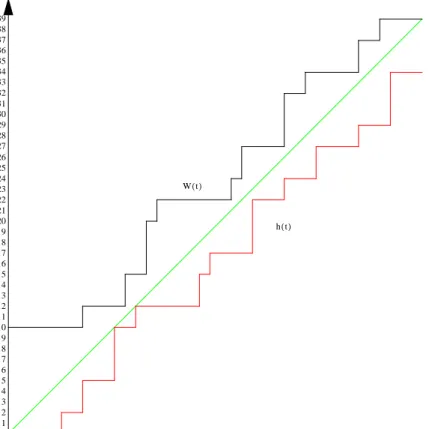
given a critical instant at time 0 ( , ), the workload is the amount of processing time requested by all activations whose release times are in the interval [BMR90]:

•

given a critical instant at time 0 ( , ), the processor demand is the amount of computation time requested by all activations whose release times and absolute deadlines are in the interval [BMR90],[SPU96]:

.

U

≤

c

<

1

c

U

C

j

T

_j ---j=1 n

∑

=

U

≤

1

P

=

lcm

_{1≤ ≤i n}

{ }

T

_i

P

i

∀

∈

[

1 n

,

]

s

_i

=

0

W t( )

0 t

,

)

[

W t

( )

t

T

_j

--- C

j j=1 n

∑

=

i

∀

∈

[

1 n

,

]

s

_i

=

0

h t

( )

0 t

,

]

[

h t

( )

max 0 1

t

–

D

j

T

_j

---+

,









j=1 n

∑

C

_j

1

t

–

D

j

T

_j

---+









Dj≤t

∑

C

_j

=

=

•

: Given a non-concrete task set, the synchronous processor busy period is defined as the time interval delimited by two distinct processor idle periods1 in the schedule of the corresponding synchronous concrete task set (where 0 is a critical instant, i.e., , ). It turns out that the value of does not depend on the scheduling algorithm, as far as it is non-idling, but only on the task arrival pattern. Note that (cf. Appendix A, page 120, and Appendix B, page 127, for a more formal discussion):

-

can be computed recursively using the workload [KLS93]2.

-

in the sequel, we will see how it is possible to generalize the concept of Busy period with respect to a fixed or dynamic priority (let denotes, for task , the maximum interval of such a priority busy period). It turns out that the value of depends on the scheduling algorithm.

•

Given a non-concrete general task , , is the worst-case response time of , i.e., the longest time ever taken by any activation of the task from its release time until the time it completes its required computation [JP86]. Note that:

-

as shown in the sequel, the value of is scheduling algorithm dependent and can be computed using the concept of priority busy period.

-

if a task has a worst-case response time greater than its period then there is the possibility for a task to re-arrive before the previous activations have completed. In our model, we consider that the new arrival is delayed from being executing after the previous activation terminate. In other words we keep the order of the events of the same task. Other ways to deal with such a situation exist (e.g. to deliver the most recent activation of the same task first), leading to an adaptation of the proposed results.

1.2 Previous work

Given a scheduling context, the main goal of the existing results is to couple an optimal scheduling algorithm with a polynomial-time or pseudo-polynomial-time (in order to be practical) Feasibility Condition (FC) that could be either Sufficient Condition (SC) or Necessary and Sufficient Condition (NSC). An FC can lead either to establish the feasibility only of the given real-time problem, or to extra informations as the worst-case response time of any task (in both cases, the proofs require to identify the worst pattern(s) of arrival). As said previously, the community of real-time researchers is currently split in two camps, those who support fixed priority driven scheduling algorithms (whose main results are presented in Section 1.2.2, page 18) and those who support dynamic priority driven scheduling algorithms (whose main results are presented in Section 1.2.1, page 12). Note that:

•

the proposed state-of-the-art are not an exhaustive list of the papers related to real-time scheduling but more a summary of the main steps and new approaches proposed in this field (see [GRS96] for a more detailled state-of-the-art).

•

the given theorems are adapted to take into account our notations.

1. A processor idle period can have a zero duration when there is only one outstanding computation and the end of this computation coincides with a new request of a new one.

2. The recursion ends when and can be solved by successive iterations starting from . Indeed, it is easy to shown that is non decreasing. Consequently, the series converges or exceeds if , in the latter case, the task set is not schedulable. Finally, this kind of recursive expression is pseudo-polynomial if .

λ

0

,

λ )

[

i

∀

∈

[

1 n

,

]

s

_i

=

0

λ

λ

λ

k+1

W

( )

λ

k

λ

k

λ

=

=

=

λ

0

W 0

( )

+

=

λ

k

P

U

>

1

U

≤

c

<

1

λ

_i

τ

_i

λ

_i

τ

_i

∀

i

∈

[

1 n

,

]

r_i

τ

_i

r

_i

1.2.1 Dynamic priority driven scheduling algorithms

In this section, we briefly summarize the principles of preemptive, non-idling dynamic priority scheduling. These principles were derived in particular from [LL73], [LM80], [BMR90], [BHR93], [KLS93], [ZS94], [SPU96], [RCM96] and [GRS96].

1.2.1.1 Optimality

We will focus on the EDF (Earliest Deadline First) scheduling algorithm. At any time, EDF executes among those tasks that have been released and not yet fully serviced (pending tasks), one whose abso-lute deadline is earliest. If no task is pending, the processor is idle.

Theorem 1 -

([DER74]) EDF is optimal.

The proof shows that it is always possible to transform a valid schedule to one which follows EDF. More precisely, if at any time the processor executes some task other than the one which has the earliest absolute deadline, then it is possible to interchange the order of execution of these two tasks (the resul-ting schedule is still valid).

Note that the optimality property of EDF is more general than the optimality property of any fixed prio-rity driven scheduling algorithms. Indeed, EDF is said to be optimal in the sense that no other dynamic, as well as fixed, priority driven scheduling algorithm can lead to a valid schedule which cannot be obtained by EDF. This ambiguity on the concept of optimality will be overcome in Section 2.1, page 24, with respect to the concepts of scheduling referential andΣ-optimality.

Note also that, exept EDF and LLF1, there is no other optimal scheduling algorithm, in our knowledge for the dynamic case. Consequently, in the sequel, all the results (in particular the complexity analysis of the feasibility conditions) described for that case are referred to EDF. We are fully aware that a for-mal justification of this choice has to be done but we let that point as an open question for the interested reader.

1.2.1.2 Feasibility

■ Case ,

Theorem 2 -

([LL73]) For a given synchronous periodic task set (with

,

), the EDF schedule is feasible if and only if

.

This result gives us a simple O(n) procedure based on the processor utilization to check the feasibility. The proof shows that if a given processor busy period leads to an overflow at time t, the resulting syn-chronous processor busy period cannot lead to an idle time prior to time t. This leads to a contradiction if we assume and an overflow at time t.

Theorem 3 -

([LL73], [KLS93]) Any non-concrete periodic task set (with

,

) scheduled by EDF, is feasible if and only if no absolute deadline is missed during the

synchronous busy period.

This result is related to the previous theorem. That is, if an absolute deadline is missed in a given busy period, then one is missed in the synchronous processor busy period.

1. The LLF (Least Laxity First) scheduling algorithm, which at any scheduling decision chooses the task activa-tion with the smallest laxity (absolute deadline minus current time minus remaining execuactiva-tion time) has also been shown to be optimal in the same context [MOK83] but leads to more preemptions than EDF and worst response times. Consequently, it has received less attention in the literature.

i

∈

[

1 n

,

]

∀

T

_i

=

D

_i

i

∈

[

1 n

,

]

∀

T

_i

=

D

_i

U

≤

1

U

≤

1

i

∈

[

1 n

,

]

∀

T

_i

=

D

_i

■ Case , .

Historically, a NSC for this model has been known since the publication of [LM80] (improved latter by [BHR90]), in which Leung and Merril established that the feasibility of an asynchronous task set can be checked by examining the feasibility of the EDF schedule in the time interval

(with and as defined in Section 1.1, page 8).

Note that this NSC operates in exponential time in the worst-case (which is usually unacceptable) since is in the worst case a function of the product of the task periods. It turns out that for a synchronous periodic task set we can restrict our attention to the interval , with a critical instant. That is, the synchronous arrival pattern is the most demanding for non-concrete task set.

In addition to these results, the approach we are going to show now is based on the evaluation of the processor demand on limited intervals such as the synchronous processor busy period (cf. Section 1.1.2, page 10). Indeed, being the processor demand, the amount of computation requested by all activations in the interval , it follows that for any , must not be greater than in order to have a valid schedule. Note that this approach leads to a pseudo-polynomial NSC if (i.e. with c a constant smaller than one).

Theorem 4 -

([BRH90], [BMR90], [ZS94],[RCM96]) A non-concrete periodic, or

sporadic, task set (with

and

) is feasible, using EDF, if and only if:

, (1)

where

and is the length of the synchronous processor busy period (cf. Section 1.1.2, page 10).

This theorem unifies several results. A first improvement on the result of [LM80] for synchronous periodic task sets is found in [BHR90] and [BMR90], where Baruah et al. show that if an NSC for the feasibility of a task set is that , in the limited interval:

The proof is based on the fact that if the task set is not feasible, then there is an instant of time such that . By algebraic manipulations of this condition, an upper bound on the value of can be determined. Recently, by using a similar manipulation on the same condition, [RCM96] obtained a tighter upper bound:

If there is (with since , ), then we have:

from which:

i

∈

[

1 n

,

]

∀

D

_i

≤

T

_i

0 2P

,

+

max s

{ }

_i

[

]

P

s

_i

P

0 P

,

[

]

0

h t

( )

0 t

,

[

]

t

≥

0

h t

( )

t

U

≤

c

<

1

D

_i

≤

T

_i

∀

i

∈

[

1 n

,

]

U

≤

1

t

∀

∈

S

h t

( )

≤

t

S

{

kT

_j

+

D

_j

,

k

∈

IN

}

j=1 n

∪









_{0 min}

_λ

_j=1

(

1

–

D

j

⁄

T

j

)

C

j n

∑

1

–

U

---,













,







,

∩

=

λ

U

<

1

t

∀

h t

( )

≤

t

0

U

1

–

U

--- max

_i=1…n

(

T

_i

–

D

_i

)

,

_



.

t

h t

( )

>

t

t

t

<

h t

( )

h t

( )

1

t

–

D

j

T

_j

---+









j=1 n

∑

C

_j

=

∀

i

∈

[

1 n

,

]

D

_i

≤

T

_i

t

<

h t

( )

t

+

T

j

–

D

j

T

_j

---







_C

j j=1 n

∑

tU

1

D

j

T

_j

---–









_C

j j=1 n

∑

+

,

=

≤

t

1

–

D

_j

⁄

T

_j

(

)

C

_j j=1 n

∑

1

–

U

---.

<

Note that if , with a constant smaller than 1, this result leads to a pseudo-polynomial-time NSC [BRM90]. Note also that the interval to be checked can be large if is close to 1.

A second upper bound on the length of the interval to be checked is given in [SPU95], [RCM96]. In particular, Ripoll et al. extend to , , the result of Theorem 3, page 12, by showing that the synchronous processor busy period is the most demanding one (using the same overflow argu-ment as in [LL73]). That is, if an absolute deadline is missed in the schedule, then one is missed in the synchronous processor busy period.

Finally, the evaluation of the NSC is further improved as proposed by [ZS94], who propose to evaluate the processor demand only on the set S of points corresponding to absolute deadlines of task requests (i.e. the set of points where the value of changes).

■ Case ,

Theorem 5 -

([BMR90]) A non-concrete periodic, or sporadic, task set (with

,

) is feasible, using EDF, if and only if

.

The proof of [BMR90] simply shows that if , and :

,

from which: .

■ General task sets ( , and are not related)

The results seen for task sets with relative deadlines smaller than or equal to the respective periods, are also valid for general task sets, in which there is no a priori relation between relative deadlines and periods. In particular, Theorem 3, page 12, originally conceived for task sets with relative deadlines equal to periods, was independently shown (by [RCM96] and [SPU95, SPU96], respectively) to hold also for the less restrictive models. That is, in order to check the feasibility of a general task set, we still can limit our attention to the synchronous busy period. [GRS96] defined a more specialized notion of busy period, namely the deadline busy period, that enables us to refine the analysis by further restricting the interval of interest.

Definition 1 -

([GRS96]) A deadline- busy period is a processor busy period in which only

task activations with absolute deadline smaller than or equal to execute.

It turns out that only synchronous deadline busy periods are the busy periods interesting in order to check the feasibility of task set since they derived the following property:

Lemma 1 -

([GRS96]) Given a general task set, if there is an overflow for a certain arrival pattern,

then there is an overflow in a synchronous deadline busy period

.

The proof is still an extension of Theorem 3, page 12, showing that if a given processor busy period leads to an overflow at time , the resulting synchronous deadline- busy period leads also to an

over-U

≤

c

c

c

i

∈

[

1 n

,

]

∀

D

_i

≤

T

_i

h t

( )

i

∈

[

1 n

,

]

∀

D

_i

≥

T

_i

i

∈

[

1 n

,

]

∀

D

_i

≥

T

_i

U

≤

1

D

_i

≥

T

_i

∀

i

∈

[

1 n

,

]

U

≤

1

t

≥

0

∀

h t

( )

max 0 1

t

–

D

j

T

_j

---+

,









j=1 n

∑

C

_j

1

t

–

D

j

T

_j

---+









Dj≤t

∑

C

_j

=

=

t

≥

0

∀

h t

( )

t

+

T

j

–

D

j

T

_j

---







Dj≤t

∑

C

_j

t

C

j

T

_j

---j=1 n

∑

t

≤

≤

≤

i

∀

∈

[

1 n

,

]

T

_i

D

_i

d

d

d

d

flow. Note that [GRS96] proposed an algorithm to compute , the longest synchronous deadline busy period for any task and that the synchronous processor busy period being the largest busy period, it

is possible to maximise by .

On the other hand [BHR93] and [ZS94] showed by algebraic manipulationst of , as for Theorem 4, page 13, the possibility of checking the feasibility of a general task set on the following set of points in a limited interval. The only difference with this theorem comes from the lower bound that is needed to take into account due to relative deadlines greater than periods. Finally:

[ZS94] derived from this result an admission control procedure meaning that if a general task set of n-1 tasks is feasible, it is then possible to determine the minimum value of the relative deadline for an nth task such that all the general task set of n tasks is still feasible.

Finally, as [RCM96], in the case where , [GRS96] integrated these upper bound in one NSC for general task sets.

Theorem 6 -

([BHR93], [ZS94], [RCM96], [SPU96], [GRS96]) Any general task set with

is feasible, using EDF, if and only if:

, (2)

where ,

and .

is the length, for task , of its synchronous deadline busy period and the length of the synchro-nous processor busy period (cf. Section 1.1.2, page 10).

1.2.1.3 Worst-case response time

Contrary to what happens in fixed priority systems, the worst-case response times of a general task set scheduled by EDF are not necessarily obtained with a synchronous pattern of arrival. [GRS96] showed the following lemma.

Lemma 2 -

([GRS96]) the worst-case response time of a task is found in a deadline busy period

for in which all tasks but are released synchronously from the beginning of the deadline busy period and at their maximum rate

.

λ

_is

τ

_i

λ

_is

_λ

h t

( )

S

max D

( )

_i

S

kT

_j

+

D

j

,

k

∈

N

{

}

j=1 n

∪









_{0 max max}

j=1…n

( )

D

j

1

–

D

_j

⁄

T

_j

(

)

C

_j j=1 n

∑

1

–

U

---,













,







.

∩

=

D

_i

≤

T

_i

∀

i

∈

[

1 n

,

]

U

≤

1

t

∀

∈

S

h t

( )

≤

t

S

kT

_j

+

D

j

k

0

λ

s_j

D

_j

–

T

_j

---,

∈

,













j=1 n

∪













0 min

,

{

λ

,

B

₁

,

B

₂

} ]

[

∩

=

B

₁

1

–

D

_j

⁄

T

_j

(

)

C

_j Dj≤Tj

∑

1

–

U

---=

B

₂

max max

_j=1…n

( )

D

_j j=1

(

1

–

D

j

⁄

T

j

)

C

j n

∑

1

–

U

---,













=

λ

s_j

_τ

i

λ

τ

_i

τ

_i

τ

_i

In practice (see [SPU96]), in order to find , the worst-case response time of , we need to examine several scenarios in which has an activation released at time , while all other tasks are released synchronously ( , ). Given a value of the parameter , the response time of the ’s

activation released at time is where is the length of the busy

period that includes this ’s activation. is computed by means of the following iterative computation:

, ,

where takes into account, for each task but , the number of instances released within [0,t) and having an absolute deadline smaller or equal to , i.e.:

[SPU96] first established this result showing that Lemma 2, page 15, holds if the busy period mentioned in the lemma is a processor busy period. Similarly to what was done in the previous section for the establishment of a task set feasibility, [GRS96] improved the result of [SPU96] by using the notion of deadline busy period. Indeed, the worst-case response time of is always found in a deadline busy period for (in the contrary, we have that cannot lead to a worst case response time for ). Therefore, considering Lemma 2, page 15’s patterns of arrival, [GRS96] gave an algorithm that compute , the maximum length of a synchronous deadline busy period for any task and showed that . Note that the synchronous processor busy period being the largest busy period, it is possible to maximise by .

According to Lemma 2, page 15, and to the successive considerations, the significant values of the parameter are in the interval . Furthermore, also within this interval we can restrict our attention to the points where either or coincides with the absolute deadline of another activation, which correspond to local maxima of . That is, , where:

.

Finally, a general task set is feasible, using EDF, if and only if:

, . (3)

The complexity of this worst-case response time analysis will be detailled in the sequel and compared with the fixed priority case.

r

_i

τ

_i

τ

_i

a

s

_j

=

0

∀

j

≠

i

a

τ

_i

a

r

_i

( )

a

=

max C

{

_i

,

L

_i

( )

a

–

a

}

L

_i

( )

a

τ

_i

L

_i

( )

a

L

_i( )0

_{( )}

_a

₌

₀

_L

i(k+1)

( )

a

=

W

i

(

a L

,

i( )k

( )

a

)

+

(

1

+

a T

⁄

i

)

C

i

W

_i

(

a t

,

)

τ

_i

a

+

D

_i

W

_i

(

a t

,

)

min

t

T

_j

---

1

a

+

D

i

–

D

j

T

_j

---+

,













C

_j

.

j≠i Dj≤a+Di

∑

=

τ

_i

τ

_i

L

_i

( )

a

–

a

<

0

τ

_i

λ

_i

τ

_i

D

_i

≤

D

_j

⇒

λ

_i

≤

λ

_j

λ

_i

λ

a

[

0

,

λ

_i

]

s

_i

=

0

a

+

D

_i

L

_i

( )

a

a

∈

A

∩

[

0

,

λ

_i

]

A

{

kT

_j

+

D

_j

–

D

_i

,

k

∈

N

}

j=1 n

∪

=

i

∀

∈

[

1 n

,

]

r

_i

max

a≥0

{

r

i

( )

a

}

≤

D

i

=

1.2.1.4 Shared resources and release jitters

For reasons such as tick scheduling or distributed contexts (e.g. the holistic approach introduced by [TC95] for fixed priority scheduling that was extended for dynamic priority scheduling in [SPU96-2], [HS96]), tasks may be allowed to have a release jitter (i.e., a task τ_i may be delayed for a maximum time before being actually released). In such case, if a task is delayed for a maximum time before being actually released, then two consecutive instances of may be separated by the interval

.

Furthermore, if the tasks are allowed to share resources, the analysis must take into account additional terms, namely blocking factors, because of inevitable priority inversions. Note that:

•

the maximum duration of such inversions can be bounded if shared resources are accessed by locking and unlocking semaphores according to protocols like the priority ceiling [CL90], [RSL90] or the stack resource algorithm [BA91]. In particular, for each taskτ_i it is possible to compute the worst-case blocking time B_i. For example, the priority ceiling of a semaphore is defined as the priority of the highest priority task that may lock that semaphore. A taskτ_i is then allowed to enter a critical section if its priority is higher than the ceiling priorities of all the semaphores locked by task other thanτ_i. The task will run at its assigned priority unless it is in a critical section and blocks higher priority tasks. In the latter case, it must inherit the highest priority of the tasks it blocks but will resume at its assigned priority on leaving the critical section.

•

the length of the processor busy periods is unaffected by the presence of blocking instead. Priority inversions may only deviate the schedule from its ordinary EDF characteristic. The required modifications on the analysis are only few. The occurrence being checked, or another one which precedes it in the schedule, may experience a blocking that has to be included as an additional term.

[SPU96] examined the feasibility of a general task sets in presence of shared resources and release jitter.

Theorem 7 -

([SPU96]) a general task set in presence of shared resources and release

jitters is feasible (assuming that tasks are ordered by increasing value of D

_i

-J

_i

), using EDF, if:

, . (4)

where is the size of the synchronous processor busy period and .

The proof generalizes Theorem 6, page 15, showing that the worst processor busy period is still the synchronous processor busy period and that the worst pattern of arrival, considering release jitter, is when tasks experience their shortest inter-release times at the beginning of the schedule. Considering shared resources, it is shown that the worst pattern of arrival arises with the blocking factors of the task with the largest value among those included in the sum. Similarly, [SPU96] develops the same arguments for the computation of the worst-case response time.

J

_i

τ

_i

J

_i

τ

_i

T

_i

–

J

_i

λ

t

∀

≤

λ

1

t

+

J

i

–

D

i

T

_i

---+









Di≤t+Ji

∑

C

_i

+

B

_{k t( )}

≤

t

λ

k t

( )

=

max k D

{

(

_k

–

J

_k

≤

t

)

}

D

_k

–

J

_k

1.2.2 Fixed priority driven scheduling algorithms

In this section, we briefly summarize the principles of preemptive, non-idling, fixed priority schedu-ling. These principles were derived in particular from [LL73], [LW82], [JP86], [LEH90], [AUD91] and [TBW94]. Note that, contrary to what is happening in the dynamic priority case, feasibility and res-ponse time computation are closely related in the state-of-the-art.

1.2.2.1 Optimality

Optimality property is limited in this section to the fixed priority driven class of scheduling algorithms. In other words, a scheduling algorithm x is said to be optimal in the sense that no other fixed priority assignment can lead to a valid schedule which cannot be obtained by x. This limitation reflects the theo-retical dominance of the class of dynamic priority driven scheduling algorithms (e.g., a NSC for fixed priority driven scheduling algorithms is a SC considering EDF). Anyhow, this ambiguity on the con-cept of optimality will be overcome in Section 2.1, page 24, with respect to the concon-cepts of scheduling referential andΣ-optimality.

In the case , , original work of [LL73] establishes the optimality of the Rate Monotonic (RM) priority ordering. The priority assigned to tasks by RM is inversely proportional to their period. Thus the task with the shortest period has the highest priority. For task sets with relative deadlines less or equal to periods, an optimal priority ordering has been shown by [LW82] to be the deadline monotonic (DM) ordering. The priority assigned to tasks by DM is inversely proportional to their relative deadline (note that DM is strictly equivalent to RM in the case , ). [LEH90] points out that neither RM nor DM priority ordering policies are optimal for general tasks set (i.e. when relative deadlines are not related to the periods). Finally, [AUD91] solves this problem giving an optimal priority assignment procedure (Audsley) in O(n2) that must be combined with the feasibility analysis presented in the sequel.

Theorem 8 -

([AUD91]) The Audsley priority assignment procedure is optimal for

general task sets.

The procedure first tries to find out if any task with an assigned priority of level n is feasible. Audley proves that if more than one task is feasible with priority level n, one can be chosen arbitrarily amoung the matching tasks. Then the first feasible task of level n is removed from the task set and priority level is decreased by one. The procedure proceeds with the new priority level until either all remaining tasks have been assigned a priority (the task set is then feasible) or for a certain priority level (no task is feasible, then there is no priority ordering for the given task set).

1.2.2.2 Feasibility condition and worst-case response time

■ Case ,

Theorem 9 -

([LL73]) For a given synchronous periodic task set (with

,

), the RM schedule is feasible if

.

[LL73] proved the sufficiency of this processor utilization test, for tasks assigned priorities according to RM, showing that it is possible to find a least upper bound on the processor utilization. This result gives us a simple O(n) procedure to check the feasibility.

i

∀

∈

[

1 n

,

]

T

_i

=

D

_i

i

∀

∈

[

1 n

,

]

T

_i

=

D

_i

i

∀

∈

[

1 n

,

]

T

_i

=

D

_i

i

∀

∈

[

1 n

,

]

T

_i

=

D

_i

U

n 2

1 n

---1

–













≤

Note that [LL73] also proposed a mixed scheduling algorithm showing that when there is a task setτ scheduled by a fixed priority scheduling algorithm and another task set τ’ scheduled by EDF in bac-kground (i.e., when the processor is not occupied by the first task set), then the availability function f(t), defined as the accumulated processor time from 0 to T available to τ’, can be shown to be sublinear,

i.e., a function for which: .

It follows that:

•

if a given processor busy period obtained by these two task sets leads to an overflow at time t, the resulting synchronous processor busy period cannot lead to an idle time prior to time t.

•

a NSC for the second task set is:

, .

where is the length of the synchronous processor busy period (cf. Section 1.1.2, page 10).

Note that the application of this result involves the resolution of a large set of inequalities and that [LL73] did not establish a closed form expression for the least upper bound on (the global processor utilization allowed for τ and τ’). They just proposed hints for simple, but pessimist, sufficient condi-tions and showed in an example that the bound on is considerably less restrictive when the number of task scheduled by EDF (rather than a fixed priority scheduling algorithm) grows.

Note also that in [LEH90], Lehoczky shows that in the particular case where periods are harmonic, a 100% processor utilization can be obtained. Other particular cases have been studied in [LEH90] using a processor utilization approach.

In addition to this first approach (based on ) another interesting approach focused on deriving the worst-case response times of each task of a given non-concrete task set. This led to the obvious following NSC that unifies the feasibility of a task set with the worst-case response times:

.

Let us summarize now the main results on the worst-case response time computation in several contexts for fixed priority driven scheduling algorithms.

■ Case ,

Theorem 10 -

([JP86]) The worst-case response time

of a task

of a non-concrete

periodic, or sporadic, task set (with

,

) is found in a scenario in which all

tasks are at their maximum rate and released synchronously at a critical instant t=0.

is

computed by the following recursive equation (where hp(i) denotes the set of tasks of higher

priority than task

):

.

Furthermore, the task set is feasible if and only if:

,

.

f T

( )

≤

f T

(

+

t

)

–

f t

( )

t

∀

≤

λ

f t

( )

t

T

_i

--- C

i τ′i∈τ′

∑

≥

λ

U

U

U

r

_i

τ

_i

i

∀

∈

[

1 n

,

]

r

_i

≤

D

_i

i

∀

∈

[

1 n

,

]

D

_i

≤

T

_i

r

_i

τ

_i

D

_i

≤

T

_i

∀

i

∈

[

1 n

,

]

r

_i

τ

_i

r

_ik+1

C

_i

r

i k

T

_j

--- C

j j∈

∑

hp i( )

+

=

i

∀

∈

[

1 n

,

]

r

_i

≤

D

_i