HAL Id: hal-00296006
https://hal.archives-ouvertes.fr/hal-00296006
Submitted on 21 Aug 2006
HAL is a multi-disciplinary open access
archive for the deposit and dissemination of
sci-entific research documents, whether they are
pub-lished or not. The documents may come from
teaching and research institutions in France or
abroad, or from public or private research centers.
L’archive ouverte pluridisciplinaire HAL, est
destinée au dépôt et à la diffusion de documents
scientifiques de niveau recherche, publiés ou non,
émanant des établissements d’enseignement et de
recherche français ou étrangers, des laboratoires
publics ou privés.
emissions from 1997 to 2004
G. R. van der Werf, J. T. Randerson, L. Giglio, G. J. Collatz, P. S.
Kasibhatla, A. F. Arellano Jr.
To cite this version:
G. R. van der Werf, J. T. Randerson, L. Giglio, G. J. Collatz, P. S. Kasibhatla, et al..
Interan-nual variability in global biomass burning emissions from 1997 to 2004. Atmospheric Chemistry and
Physics, European Geosciences Union, 2006, 6 (11), pp.3423-3441. �hal-00296006�
www.atmos-chem-phys.net/6/3423/2006/ © Author(s) 2006. This work is licensed under a Creative Commons License.
Chemistry
and Physics
Interannual variability in global biomass burning emissions from
1997 to 2004
G. R. van der Werf1, J. T. Randerson2, L. Giglio3, G. J. Collatz4, P. S. Kasibhatla5, and A. F. Arellano, Jr.5,*
1Department of Hydrology and Geo-Environmental Sciences, Faculty of Earth and Life Sciences, Vrije Universiteit,
Amsterdam, Netherlands
2Department of Earth System Science, University of California, Irvine, California, USA
3Science Systems and Applications, Inc., NASA Goddard Space Flight Center, Greenbelt, Maryland, USA 4NASA Goddard Space Flight Center, Greenbelt, Maryland, USA
5Nicholas School of the Environment and Earth Sciences, Duke University, Durham, North Carolina, USA *now at: National Center for Atmospheric Research, Boulder, Colorado, USA
Received: 22 December 2005 – Published in Atmos. Chem. Phys. Discuss.: 18 April 2006 Revised: 14 July 2006 – Accepted: 28 July 2006 – Published: 21 August 2006
Abstract. Biomass burning represents an important source
of atmospheric aerosols and greenhouse gases, yet little is known about its interannual variability or the underly-ing mechanisms regulatunderly-ing this variability at continental to global scales. Here we investigated fire emissions during the 8 year period from 1997 to 2004 using satellite data and the CASA biogeochemical model. Burned area from 2001– 2004 was derived using newly available active fire and 500 m. burned area datasets from MODIS following the approach described by Giglio et al. (2006). ATSR and VIRS satellite data were used to extend the burned area time series back in time through 1997. In our analysis we estimated fuel loads, including organic soil layer and peatland fuels, and the net flux from terrestrial ecosystems as the balance between net primary production (NPP), heterotrophic respiration (Rh), and biomass burning, using time varying inputs of precipita-tion (PPT), temperature, solar radiaprecipita-tion, and satellite-derived fractional absorbed photosynthetically active radiation (fA-PAR). For the 1997–2004 period, we found that on average approximately 58 Pg C year−1 was fixed by plants as NPP, and approximately 95% of this was returned back to the at-mosphere via Rh. Another 4%, or 2.5 Pg C year−1was emit-ted by biomass burning; the remainder consisemit-ted of losses from fuel wood collection and subsequent burning. At a global scale, burned area and total fire emissions were largely decoupled from year to year. Total carbon emissions tracked burning in forested areas (including deforestation fires in the tropics), whereas burned area was largely controlled by sa-vanna fires that responded to different environmental and hu-man factors. Biomass burning emissions showed large inter-annual variability with a range of more than 1 Pg C year−1,
Correspondence to: G. R. van der Werf
with a maximum in 1998 (3.2 Pg C year−1)and a minimum in 2000 (2.0 Pg C year−1).
1 Introduction
The link between El Ni˜no – Southern Oscillation (ENSO) and the CO2growth rate variability is well established
(Ba-castow, 1976; Keeling et al., 1995) and provides a test case scenario for the effects of future climate change under warm and dry conditions. During El Ni˜no, drought in equatorial Asia and Central and South America simultaneously influ-ences fire activity, net primary production (NPP) and het-erotrophic respiration (Rh)in terrestrial ecosystems in a way that increases the growth rate of atmospheric CO2. Although
drought is known to trigger increases in fire emissions, its ef-fect on the balance between NPP and Rh remains uncertain. In temperate ecosystems, for example, warm and dry condi-tions increased rates of carbon uptake in a hardwood forest (Goulden et al., 1996), whereas a strong drought in Europe during the summer of 2003 led to carbon loss from multiple ecosystems (Ciais et al., 2005). In boreal regions, increased temperature may trigger increased soil thaw and a loss of soil carbon through increased Rh (Oechel et al., 1993; Goulden et al., 1998). In tropical regions, deep roots may enable trees to maintain high productivity during the dry season, whereas the metabolic activity of surface soil microbes are simultane-ously inhibited during these periods, lowering Rhand lead-ing to a net carbon sink (Saleska et al., 2003). Longer-term time series of flux measurements from tropical ecosystems are sparse and limit our ability to assess the effect of drought on interannual to decadal timescales.
Several recent studies provide evidence that fires account for a substantial fraction of the variability in the CO2growth
rate (Langenfelds et al., 2002; Schimel and Baker, 2002; van der Werf et al., 2004), suggesting that variations in NPP and Rhare more closely coupled than previously thought. Obser-vations from Indonesia show that fires in drained peatlands were a dominant source of emissions from this region dur-ing the 1997–1998 El Ni˜no (Page et al., 2002). Interannual variability (IAV) in boreal fire activity is also large (Amiro et al., 2001; Sukhinin et al., 2004) and may be linked with the Arctic Oscillation (Balzter et al., 2005), ENSO (Hess et al., 2001), temperature anomalies (Balzter et al., 2005; Flan-nigan et al., 2005), and with human activity (Mollicone et al., 2006). At a global scale, two studies have assessed inter-annual variability in biomass burning emissions on a global scale using satellite data (Duncan et al., 2003; van der Werf et al., 2004). Biomass burning estimates are uncertain but are becoming better constrained, primarily by new satellite information on burned area, improved biogeochemical mod-els used for estimating fuel loads, and atmospheric tracer in-verse modeling studies. Assuming that IAV in ocean – atmo-sphere exchange is relatively small as compared with that as-sociated with the terrestrial biosphere (Lee et al., 1998; Bat-tle et al., 2000; Bousquet et al., 2000), reliable estimates of global biomass burning emissions may help to further con-strain the climate sensitivity of processes within the terres-trial biosphere.
Fire emissions are commonly calculated as the product of burned area, fuel loads, and combustion completeness, in-tegrated over the time and space scale of interest. Burned area is usually considered to be the most uncertain param-eter in emission estimates, and burned area estimates on a global scale have only recently become available. Both the GBA2000 (Gr´egoire et al., 2002) and GLOBSCAR (Simon et al., 2004) efforts have yielded burned area estimates for the year 2000. The algorithms used in both projects were recently combined to estimate burned area over a longer time series in the GLOBCARBON initiative (Plummer et al., 2006). Other approaches to estimate burned area on large scales rely on the detection of active fires (fire counts) and relationships between these fire counts and burned area (van der Werf et al., 2003; Giglio et al., 2006). More detailed in-formation on burned area is available for specific regions, and provides a basis for validating burned area algorithms devel-oped at a global scale. Sukhinin et al. (2004) for example, estimated burned area for the 1995–2002 period for Russia using AVHRR data, and estimates of Canadian burned area from the Canadian Forest Service provide the longest time series of burned area available (Stocks et al., 2002). Fuel loads are the next most uncertain parameter required for es-timates of fire emissions. Historically, biome-averaged val-ues were used, but more recently satellite imagery has been used to represent heterogeneity within biomes (e.g., Scholes et al., 1996; Barbosa et al., 1999). Currently, most studies employ biogeochemical models to more accurately estimate
fuel loads. This approach allows for a more direct compar-ison of aboveground biomass levels estimated by the model with spatially explicit maps generated from remote sensing and field based studies (e.g., Houghton et al., 2001; Saatchi et al., 2001; Le Toan et al., 2004). Use of biogeochemical models also enables the incorporation of process-level infor-mation on herbivory and fuel wood collection that are impor-tant controllers of fuel levels and will likely respond to global change processes and growing populations over the next sev-eral decades. The Lund-Potsdam-Jena (LPJ) model has been used in several studies to estimate emissions, including esti-mating contemporary levels (Hoelzemann et al., 2004) and emissions during the Last Glacial Maximum (Thonicke et al., 2005). We previously implemented a fire module in the Carnegie-Ames-Stanford-Approach (CASA) model to esti-mate contemporary patterns of tropical fire emissions (van der Werf et al., 2003), global variations in fire emissions over an ENSO cycle (van der Werf et al., 2004), and the effect of variable burning in C3 and C4 ecosystems on
at-mospheric δ13CO2(Randerson et al., 2005). Regional-scale
models have been employed to improve emissions predic-tions from boreal regions, including the combustion of be-lowground fuels (Kasischke et al., 2005). Recent work indi-cates that the burning of belowground fuels may also be an important source of emissions in tropical regions (Page et al., 2002). Vast amounts of peat have been drained in Indonesia and are vulnerable to fire during droughts, which happened during the 1997–1998 El Ni˜no, releasing large quantities of carbon to the atmosphere (Page et al., 2002).
Only a fraction of the available fuel load is consumed dur-ing a fire event, and this fraction is represented within models by combustion completeness (CC). CC has been measured in the field for various biome and fuel types (e.g., Carvalho et al., 1995; Shea et al., 1996; Hoffa et al., 1999), and varies over the course of the fire season with more complete com-bustion at the end when fuels have had more time to dry out, as shown by Hoffa et al. (1999) for savanna ecosys-tems. In general, fine and dry fuels burn more completely than coarse and wet fuels, although a paucity of data makes it challenging to quantitatively link CC with climate in global models. Although significant effort has been made to im-prove burned area and fuel estimates, uncertainties are still large and difficult to quantify, particularly in tropical for-est biomes. Eliminating the need for explicit knowledge of burned area, fuel loads, and CC, Wooster (2002), Roberts et al. (2005), and Ichoku et al. (2005) have shown for selected regions that satellite-derived fire radiative energy can be used to directly estimate emissions, potentially providing an inde-pendent quantification of emissions.
New studies employing inverse modeling techniques com-bined with atmospheric measurements of trace gases al-low for an independent estimate of biomass burning emis-sions, and progress has been made in identifying deficien-cies of current bottom-up estimates. To better constrain biomass burning estimates, comparisons with measurements
of atmospheric CO have proven especially useful since biomass burning is a major source of CO and is responsi-ble for almost all of its interannual variability (Novelli et al., 2003; van der Werf et al., 2004). Arellano et al. (2004) used data from the Measurements Of Pollution In The Tro-posphere (MOPITT) sensor to demonstrate that inventories underestimated fossil fuel emissions from Asia, and identi-fied several areas where our previous estimates of biomass burning emissions were inadequate. In a similar study that also examined seasonal patterns, P´etron et al. (2004) demon-strated that MOPITT observations provided additional con-straints on the seasonal timing of fire emissions in the South-ern Hemisphere, especially in southSouth-ern Africa.
Here we estimated biomass burning emissions on a global scale over the 1997–2004 period. We used the satellite-driven CASA biogeochemical model (Potter et al., 1993; Field et al., 1995; Randerson et al., 1996) that was previ-ously modified to account for fires (van der Werf et al., 2003), in combination with a burned area time series derived from the MODIS sensors (Giglio et al., 2006). We extended the burned area time series back in time before MODIS using data on fire activity from Arino et al. (1999) and Giglio et al. (2003b). Our overall goal was to improve global biomass burning estimates, with specific objectives to better represent fuel loads in the boreal ecosystems and in global wetlands by modeling the burning of organic soil layers and peat, to improve the seasonality of emissions in regions where in-verse studies indicated that forward modeling estimates may inadequately represent regional dynamics, and to analyze the relation between burned area and emissions on a global scale.
2 Methods
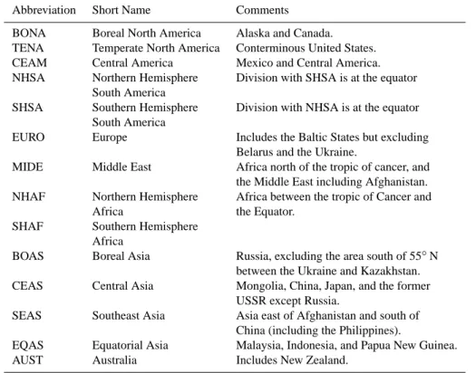
2.1 Burned area for the MODIS period (2001–2004) For our analysis, we used the burned area data set devel-oped by Giglio et al. (2006). Burned area was mapped at 500×500 m. spatial resolution within 52 globally-distributed MODIS tiles, with each tile covering an area of approxi-mately 10◦×10◦, for different time periods between 2001 and 2004 (Giglio et al., 20061). MODIS fire counts (Giglio et al., 2003a) were then calibrated to the 500-m burned area within 1◦×1◦grid cells on a monthly basis, taking advantage of additional information about fire cluster size, fractional woody cover, herbaceous cover, or bare ground (Vegetation Continuous Fields, VCF; Hansen et al., 2003), and fire per-sistence. A unique regression tree was produced for each region shown in Fig. 1. The coefficients derived from the regression trees were then used with the MODIS fire count time series to generate global monthly burned area estimates from January 2001 through December 2004. The selection of regions shown in Fig. 1 and Table 1 was based on
similar-1Giglio, L., et al.: in preparation, 2006.
46 Figure 1. Map of the 14 regions used in this study. Abbreviations are explained in Table 1. Fig. 1. Map of the 14 regions used in this study. Abbreviations are
explained in Table 1.
ities in fire behaviour and also on suitability for use as basis regions in atmospheric tracer inversion studies.
2.2 Burned area prior to the MODIS period
The Terra satellite that carried the first MODIS sensor was launched in December of 1999, but here we only used ob-servations starting in January 2001 because of inconsistent calibration during the first year of operation. The 1997–2000 period included the strongest El Ni˜no of the century associ-ated with high fire emissions so we were motivassoci-ated to extend our analysis back to include this period. To extend the time series back in time to January 1997, we used fire counts from the Tropical Rainfall Measuring Mission (TRMM) – Visible and Infrared Scanner (VIRS) and European Remote Sensing Satellites (ERS) Along Track Scanning Radiometer (ATSR) sensors. VIRS observations are available for the TRMM footprint (38◦N–38◦S), starting in January 1998 (Giglio et al., 2003b). ATSR observations are available globally, start-ing in July 1996 (Arino et al., 1999).
A comparison of the MODIS burned area time series with VIRS and ATSR observations over the 2001–2003 period re-vealed two important differences between the datasets. The first was a difference in seasonality. In Southern Hemisphere tropical ecosystems, and particularly in southern Africa, VIRS fire counts peaked about two months earlier than ATSR and MODIS. Second, ATSR fire counts at the end of 2001 were anomalously low in northern Africa as compared to both VIRS and MODIS observations. Because of these dif-ferences, in Africa we chose to use VIRS to set the IAV for the 1998–2000 period (and ATSR for 1997), while maintain-ing the seasonality as averaged over the 2001–2004 period from MODIS. For all other regions we used ATSR fire counts to set both the seasonal cycle and IAV. The procedure used to convert VIRS or ATSR fire counts to burned area was based on an analysis of the 2001–2003 MODIS overlap period. For each grid cell the 2001–2003 cumulative burned area for the three years derived from MODIS was divided by the cumula-tive VIRS/ATSR fire counts. The ratio represents the burned area per VIRS/ATSR fire count and was used to estimate
Table 1. Regions used within this study. Abbreviations refer to those used in Fig. 1.
Abbreviation Short Name Comments
BONA Boreal North America Alaska and Canada. TENA Temperate North America Conterminous United States. CEAM Central America Mexico and Central America. NHSA Northern Hemisphere Division with SHSA is at the equator
South America
SHSA Southern Hemisphere Division with NHSA is at the equator South America
EURO Europe Includes the Baltic States but excluding Belarus and the Ukraine.
MIDE Middle East Africa north of the tropic of cancer, and the Middle East including Afghanistan. NHAF Northern Hemisphere Africa between the tropic of Cancer and
Africa the Equator.
SHAF Southern Hemisphere Africa
BOAS Boreal Asia Russia, excluding the area south of 55◦N between the Ukraine and Kazakhstan. CEAS Central Asia Mongolia, China, Japan, and the former
USSR except Russia.
SEAS Southeast Asia Asia east of Afghanistan and south of China (including the Philippines).
EQAS Equatorial Asia Malaysia, Indonesia, and Papua New Guinea.
AUST Australia Includes New Zealand.
47
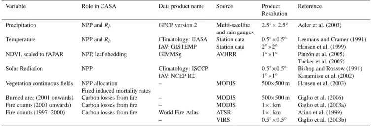
0.4 0.8 1.2 1.6 2.0 2.4 2.8 0 200 400 600 800 1000 1200 1400 NPP (g C m −2 yr −1 )Mean Annual Precipitation (m yr −1)
ORNL
CASA
Figure 2. Comparison of net primary production (NPP) estimated from the CASA model
(used here) and measurements from the Oak Ridge National Laboratory (ORNL) NPP
database. Error bars indicate the standard deviation. Measurements and model estimates are
aggregated into 200 mm year
-1bins of mean annual precipitation.
Fig. 2. Comparison of net primary production (NPP) estimated from the CASA model (used here) and measurements from the Oak Ridge National Laboratory (ORNL) NPP database. Error bars indi-cate the standard deviation. Measurements and model estimates are aggregated into 200 mm year−1bins of mean annual precipitation.
burned area from VIRS/ATSR fire counts before the MODIS era. In grid cells where no fire counts and burned area were observed in the MODIS era but fire counts were observed by
VIRS/ATSR before the MODIS era, the weighted ratio from neighbouring grid cells was used. Our approach to estimate burned area may introduce biases because of the use of dif-ferent sensors at the beginning and end of the time series, and ideally we would like to use a temporally consistent satellite-derived burned area time series. Other uncertainties in our approach are related to the ATSR algorithm which is based on detecting fires at night. It may therefore have limited suc-cess in detecting fires in high latitudes that burn around sum-mer solstice, and may have a bias towards large fires that burn into the night (Kasischke et al., 2003). However, until high quality burned area data become available, we believe our approach may serve as an interim solution in the con-text of exploring interannual variations of biomass burning emissions.
2.3 Fuel loads
For each month and grid cell, fuel loads were calculated based on the fuel load of the previous month, input from NPP, and losses from Rh, fire, fuel wood collection, and herbivory. NPP was calculated using satellite-based mea-surements of the Normalized Difference Vegetation Index (NDVI) from the Advanced Very High Resolution Radiome-ter (AVHRR) data processed by the Global Inventory Model-ing and MappModel-ing Studies (GIMMS) lab, version “g” (Pinz´on et al., 2005; Tucker et al., 2005). NDVI was converted to
fraction absorbed photosynthetic active radiation (fAPAR, see below), and NPP was calculated following the approach described by Field et al. (1995):
NPP = fAPAR × PAR × ε(T ,P ) (1)
where PAR is photosynthetically active radiation, and ε is the maximum light use efficiency (LUE) that is downscaled when temperature (T ) or moisture (P ) conditions are not op-timal. See Table 2 for a summary of the different data sources that we used to drive CASA. We converted NDVI to fAPAR using techniques developed by Los et al. (2000). Monthly PAR was derived by adding anomalies from release 2 of the National Centers for Environmental Prediction (NCEP) re-analysis data (Kanamitsu et al., 2002) to average monthly PAR derived from Bishop and Rossow (1991).
Interannually varying fAPAR was used to calculate NPP for grid cells receiving less than 1000 mm year−1 of mean
annual PPT (MAP). Otherwise the monthly mean for the study period was used. This was done because for higher MAP regions (more productive, higher NPP) IAV was rel-atively low and may not exceed uncertainties in the NDVI observations caused by residual signals from cloudiness and smoke. For all grid cells interannually varying PAR, T , and PPT were used to calculate monthly NPP. A comparison be-tween CASA NPP and results from the Oak Ridge National Laboratory (ORNL) data base (Olson et al., 2001; Zheng et al., 2003) is shown in Fig. 2 as a function of MAP. At high PPT levels, CASA NPP levels off and may slightly decrease in a way that is consistent with observations. Mechanistically both nutrient limitation and light limitation have been pro-posed as limits on NPP in these mesic environments (Schuur, 2003), although with the version of CASA used in this study light limitation was solely responsible for the model trend.
In CASA, NPP was distributed to live biomass pools (leaves, fine roots, and stems). Stems had a fixed turnover time depending on biome type. Leaf and fine root senescence depended on the seasonality of satellite-derived Leaf Area Index (LAI), with the largest transfer to heterotrophic pools occurring when LAI declined (Randerson et al., 1996). Each litter and soil organic matter pool had a maximum decom-position rate constant assigned that was reached only when soil moisture and temperature levels were not limiting. The temperature sensitivity of Rh was based on a Q10 value of
1.5. The moisture scalar was based on a simple bucket soil moisture scheme that was a function of monthly PPT, T , and soil parameters including soil texture and moisture holding capacity. Rh was limited when soil moisture was low, but also saturated soils caused a decrease in Rh rates (Potter et al., 1993).
For each grid cell, we separately calculated the carbon ex-change of herbaceous and of woody vegetation. NPP was allocated evenly to fine roots and leaves for herbaceous veg-etation, and evenly to fine roots, leaves, and stems for woody vegetation. The total grid cell carbon fluxes were then cal-culated from the proportional coverage of herbaceous and
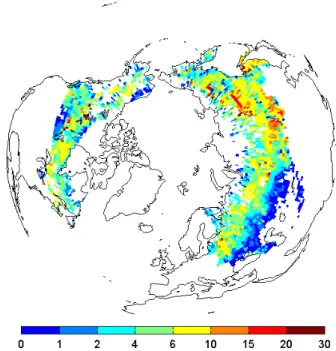
48 Figure 3. Depth of burning (cm) into the duff layer predicted by our model. Litter, coarse woody debris, and organic soil carbon consumed during fire were converted into burn depths using the soil carbon density profiles from Carrasco et al. (2006).
Fig. 3. Depth of burning (cm) into the duff layer predicted by our model. Litter, coarse woody debris, and organic soil carbon con-sumed during fire were converted into burn depths using the soil carbon density profiles from Carrasco et al. (2006).
woody vegetation determined from the VCF. We estimated fuel wood collection and herbivory as in van der Werf et al. (2003). The main result of including these two processes was a decrease in fuel loads in savanna ecosystems, in better agreement with measured fuel loads (e.g., Shea et al., 1996; Hoffa et al., 1999). Within tropical forest ecosystems, above-ground biomass levels from the model were broadly consis-tent with published estimates. For example, published esti-mates of aboveground biomass levels for the Brazilian Ama-zon range from 39 to 93 Pg C, with a mean of 70 Pg C and a standard deviation of 16 Pg C (Houghton et al., 2001). Here we estimated a total of 77 Pg C using CASA for this same region. In the future, satellite or aircraft based estimates of vegetation height may enable a further reduction in uncer-tainties in aboveground biomass estimates.
In the boreal region, a large fraction of fire emissions comes from the combustion of organic soils and peat. Re-cent research in Indonesia has also highlighted the impor-tance of peat as fuel for combustion in tropical regions. The Indonesia case is unique in that peat deposits have been sys-tematically drained and thus have become vulnerable to fire during periods of drought (Page et al., 2002). Modeling the combustion of the organic soil layer and peat is problematic because little information on depth of burning is available. Here we implemented a parameterization for boreal forest and tropical peatland soils that builds on the work of Ito and Penner (2004) and Kasischke et al. (2005). Within the CASA
Table 2. Data sets used in this study.
Variable Role in CASA Data product name Source Product Reference Resolution
Precipitation NPP and Rh GPCP version 2 Multi-satellite 2.5◦×2.5◦ Adler et al. (2003)
and rain gauges
Temperature NPP and Rh Climatology: IIASA Station data 0.5◦×0.5◦ Leemans and Cramer (1991)
IAV: GISTEMP Station data 2◦×2◦ Hansen et al. (1999) NDVI, scaled to fAPAR NPP, leaf shedding GIMMSg AVHRR 1◦×1◦ Pinz´on et al. (2005)
Tucker et al. (2005) Solar Radiation NPP Climatology: ISCCP 0.5◦×0.5◦ Bishop and Rossow (1991)
IAV: NCEP R2 1◦×1◦ Kanamitsu et al. (2002) Vegetation continuous fields NPP allocation – MODIS 500×500 m Hansen et al. (2003)
Fired induced mortality rates
Burned area (2001 onwards) Carbon losses from fire – MODIS 500×500 m Giglio et al. (2006) Fire counts (2001 onwards) Carbon losses from fire – MODIS 1×1 km Giglio et al. (2003a) Fire counts (1997–2000) Carbon losses from fire World Fire Atlas ATSR 1×1 km Arino et al. (1999)
– VIRS 0.5◦×0.5◦ Giglio et al. (2003b)
framework, the spatial variability of carbon in the organic soil layer and peat is a function of local NPP and decomposi-tion rates, with turnover times for different soil carbon pools scaled by monthly temperature and soil moisture. We ad-justed the decomposition rate constants of the deeper, slowly decaying soil carbon pools (slow and passive pools) in the CASA framework so that the modelled estimates of total soil and surface carbon in boreal and peat regions matched mea-sured values from Batjes (1999) to a depth of 30 cm. The database compiled by Batjes (1999) is based on more than 4000 globally distributed soil profiles and has a 0.5◦×0.5◦ spatial resolution. As a result, the largest adjustments to the decomposition rate constants were made in wetland areas, where anaerobic conditions lead to slow decay of carbon that was not previously taken into account in the model. We as-sumed that the deeper carbon in CASA (slow and passive pools) was only available as fuel in grid cells that were clsified as wetlands (Matthews and Fung, 1987) which we as-sumed to represent peatlands. In other (boreal) grid cells, only carbon stored in upper soil layers (represented in CASA by the surface litter and active soil pools) was allowed to burn.
The maximum depth that the fires could burn into the organic soil layer or peat was constrained using literature values. In the tropical peat areas the depth was set to the maximum soil depth in CASA (30 cm.), but may burn even deeper according to Page et al. (2002). In the boreal re-gions the maximum depth was 10 cm., corresponding to 1/3 of the available soil carbon in CASA (based on the “mod-erate severity scenario” in Kasischke et al. (2005) and ref-erences therein). Not all of the organic soil layer and peat burns in a fire; often the late season fires burn deeper than early season fires because the soil is drier (Kasischke et al., 2005). Depth of burning was made a linear function of the soil moisture scalar; only when the soil was dry would the
fires burn to the maximum depth as discussed above, cor-responding to 1/3 (boreal) and all (tropical) of the available carbon in the organic soil layer or peat in CASA. The mois-ture scalar simulates the first order effects of precipitation and evapotranspiration on soil moisture conditions, but may have limited applicability in regions where other conditions, e.g. permafrost, affect the moisture conditions of the soil. In tropical peat areas, fires were assumed to always consume a minimum of 50% of the soil carbon pools in CASA (rep-resenting human-induced drainage of peatlands; Page et al., 2002). The soil moisture scalar determined how much of the remaining 50% of the soil organic layers could burn.
We assumed that the carbon density did not change with depth. Even though several field studies have shown how the carbon density increases with depth, we believe that these studies are not yet sufficiently spatially representative to be included in a global model study. To test whether our as-sumption was valid, we used the carbon density profile from Carrasco et al. (2006) to see what the depth of burning would be when we combined our modelled organic soil layer con-sumption with this profile. The Carrasco et al. (2006) carbon density profile increases from approximately 0.015 g C cm−3 at the surface to approximately 0.020 g C cm−3at 20 cm, and approximately 0.040 g C cm−3 at a depth of 40 cm. The depth of burning corresponding to losses from CASA organic soil layer and peat is shown in Fig. 3. Most of the forest fires burned to a depth of 4–10 cm. A few wetland areas had greater levels of fire severity, including fire complexes near Lake Baikal. Fires in grassland and agricultural ecosystems south of the boreal forest consumed only a few centimetres or less.
2.4 Combustion completeness
The ratio of fuel consumption to total available fuels is known as the combustion completeness (CC) or the
combustion factor. Several generalities about CC have emerged from studies that have measured CC’s in a wide range of vegetation types (e.g., Shea et al., 1996; Hoffa et al., 1999; Carvalho et al., 2001). First, CC of fine fuels is usu-ally very high, up to 1 (complete combustion) for dry surface litter. Coarser fuels such as stems and woody debris, with a lower surface to volume ratio, burn less completely. In boreal regions foliage and twigs have a higher CC than living stems and boles in part because of their high water content. Even though the boles remain largely intact, boreal fires across North America and parts of Siberia frequently cause stand-replacing mortality of the dominant conifer species. In con-trast, in savannas fire-induced mortality of most large trees is quite low because they are protected by a thick bark and be-cause ground fuels often do not produce flames high enough to reach the foliage (Gill, 1981). CC in tropical forests un-dergoing deforestation is more challenging to characterize. Carvalho et al. (2001) reported an increase in CC with an in-crease in cleared area in deforestation regions in the Brazilian state of Mato Grosso. Here, conversion is often highly mech-anized and CC can approach unity over the course of a fire season as fuels including boles are piled together and ignited multiple times (D. C. Morton and R. S. DeFries, personal communication).
In CASA, we allowed CC to vary among fuel types (leaves, stems, and various litter pools), in contrast with earlier approaches where a single value was used for each biome. We also allowed CC to vary from month to month to simulate the effects of seasonal changes in fuel moisture content (Shea et al., 1996). We set minimum and maximum values for each fuel type (Table 3), and used moisture condi-tions to scale between these values. For live material (stems, foliage), CC was scaled linearly with the CASA NPP mois-ture scalar to take into account the effects of moismois-ture con-tent of the vegetation. CC of litter was scaled using the ratio of PPT over potential evaporation of the month of the fire and the previous month. To account for a longer memory of coarse fuels due to their greater volume to surface area ratio the relative weighing of the current and previous month was 6:4 for coarse woody debris and 9:1 for fine litter fuels.
To simulate higher CC due to repetitive burning in defor-estation regions we increased the CC of stems and coarse litter in areas with high levels of fire persistence as identi-fied using the remote sensing approach described by Giglio et al. (2006). In these grid cells, the CC value was multi-plied with a factor equal to the fire persistence, with an upper threshold for CC of 1.
2.5 Emission factors
Emission factors (EF) have been measured for multiple species in laboratories, ground based field studies, and from aircraft. EF’s are usually defined as grams of trace gas emit-ted per kg of dry matter (DM) consumed during the fire. An-dreae and Merlet (2001) reviewed most of these studies and
Table 3. Minimum and maximum combustion completeness (CC) for different fuel types.
Fuel Type CCmin CCmax
Leaves 0.8 1.0
Stems 0.2 0.3
Fine leaf litter 0.9 1.0
Coarse woody debris 0.5 0.6 Organic soil layer and peat 0.9 1.0
compiled EF’s for over 100 trace gas species. EF’s were re-ported for different biomes and in general, the finer the fuel and thus the more efficient the fire, the higher the EF for CO2 and the lower the EF for most other (reduced) trace
gases. The fraction of emitted carbon that is CO2is usually
referred to as combustion efficiency (CE). EF’s are not con-stant within biomes as shown by the relatively large standard deviations reported by Andreae and Merlet (2001). One rea-son for variation within biomes may be the timing of fires; CE is usually lower in early season fires than in late sea-son fires because fuels are drier later in the seasea-son. Korontzi et al. (2003), for example, showed how the EF for CO de-creased from 100 to 40 g CO/kg DM in the first 6 weeks of a grassland fire season, while the CO2 EF increased from
1640 to 1770 g CO2/kg DM during the same period,
indi-cating an increase in CE as the dry season progressed. On the other hand, woody vegetation may not combust until the end of the dry season, potentially decreasing the seasonal trend in EF. Because of this and because of limited infor-mation on the seasonal dependence of EF in other biomes, we have used the average values of Andreae and Merlet (2001) and Andreae (personal communication) in combi-nation with the MODIS vegetation cover map (MOD12C1 with the IGBP land cover classification, available online at http://edcdaac.usgs.gov/modis/mod12c1v4.asp).
Andreae and Merlet (2001) report EF’s for tropical forest, extratropical forest, and savanna and grassland. All grid cells in class 2 (evergreen broadleaf forest) were assigned the EF for tropical forest, all grid cells in classes 1, 3, 4, and 5 (ever-green needleleaf forest, deciduous needleleaf forest, decidu-ous broadleaf forest, and mixed forest, respectively) were as-signed the EF for extratropical forest, and all other grid cells were assigned the EF for savanna and grassland. The higher EF for reduced carbon species in forests compared to savan-nas is linked with an increased fraction of coarse fuels that burn in the smouldering phase (Andreae and Merlet, 2001). In equatorial Asia, there were several savanna grid cells that had peat burning, because the Matthews and Fung (1987) maps indicated that these grid cells contained wetlands. For the combustion of the peat in these grid cells, we used the EF from tropical forest instead of savanna to account for the lower CE. Most EF’s are reported for DM, we used a dry
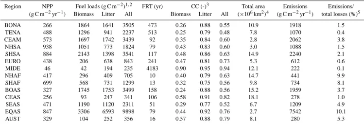
Table 4. 1997–2004 average NPP, fuel loads, fire return time (FRT), and combustion completeness (CC) for different regions.
Region NPP Fuel loads (g C m−2)1,2 FRT (yr) CC (-)3 Total area Emissions Emissions/ (g C m−2yr−1) Biomass Litter All Biomass Litter All (×106km2)4 (g C m−2yr−1) total losses (%)5 BONA 266 1864 1641 3505 473 0.26 0.88 0.55 10.9 1918 1.5 TENA 488 1296 941 2237 513 0.25 0.79 0.48 7.8 1070 0.4 CEAM 573 1697 1742 3439 92 0.35 0.84 0.60 2.8 2062 3.8 NHSA 938 1051 773 1824 79 0.43 0.83 0.60 3.0 1088 1.5 SHSA 884 2143 1398 3541 117 0.48 0.86 0.63 14.9 2240 2.1 EURO 438 206 638 843 241 0.47 0.81 0.73 5.3 612 0.6 MIDE 46 42 194 235 4183 0.90 0.95 0.94 12.1 222 0.1 NHAF 417 296 409 705 10 0.40 0.79 0.63 14.7 441 9.9 SHAF 699 568 731 1299 13 0.32 0.75 0.56 9.8 734 8.1 BOAS 327 1745 1753 3499 158 0.24 0.88 0.56 15.2 1959 3.7 CEAS 256 93 247 341 106 0.58 0.91 0.82 18.1 278 1.0 SEAS 471 1190 1120 2311 51 0.29 0.77 0.52 6.7 1209 4.9 EQAS 847 3306 6593 9898 79 0.44 0.92 0.76 2.7 7542 10.1 AUST 329 104 252 356 16 0.57 0.88 0.79 8.1 280 5.3
1Fuel loads were weighted by burned area and separated into biomass fuel (which included all live herbaceous and woody biomass available for fire) and litter fuel (aboveground litter, coarse woody debris, belowground litter in boreal regions, and belowground peat in wetland regions).
2The fraction of woody biomass that was available for fire depended on the mortality scalar, as in van der Werf et al. (2003). 3CC was weighted by burned area and by fuel loads and separated into biomass CC and litter CC similar to the fuel loads separation. 4Total surface area of the region.
5Total losses included emissions (both from vegetation fires and biofuel burning) and R
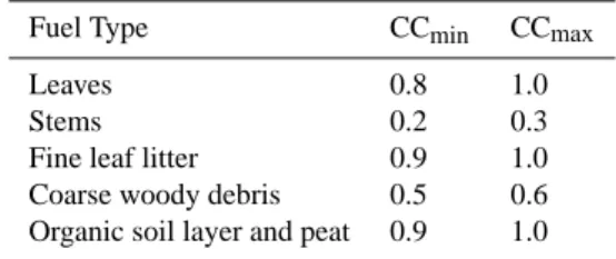
h. 97 98 99 00 01 02 03 04 2.5 3 3.5 4 Burned area (10 6 km 2 year −1 ) Emissions (Pg C year −1 )
burned area emissions a) Global 97 98 99 00 01 02 03 04 2 2.5 3 3.5 97 98 99 00 01 02 03 04 0 0.5 1 Burned area (10 6 km 2 year −1 ) Emissions (Pg C year −1 )
burned area emissions
Year b) Forests 97 98 99 00 01 02 03 04 0 1 2 Fig. 4
Fig. 4. Annual area burned and emissions for the globe (a) and for forested areas (b).
matter carbon content of 45% to convert carbon emissions to DM burned.
3 Results and discussion
3.1 Global overview
At a global scale, burned area and fire emissions were mostly decoupled over the 1997–2004 period (Fig. 4a). This was because most of the burned area occurred within savanna ecosystems that had relatively low fuel loads and emissions. Burned area within forest biomes accounted for less than 20% of global burned area averaged over the 1997–2004 pe-riod. Nevertheless, burning in forests was highly variable from year to year and this variability, coupled with high fuel loads, meant that forests contributed to most of the variability in emissions (Fig. 4b). An exception occurred in 1997, when burned area in forests was average but global emissions were high from fires in regions with tropical peatlands that have even higher fuel loads than forests (Table 4).
On average, emissions per unit burned area for the 2001– 2004 period were 2.22 kg C m−2year−1 in forest grid cells and 0.52 kg C m−2year−1in herbaceous grid cells (Fig. 5a,
Table 4). Average emissions per fire count varied somewhat less between forest (2.71×10⁶kg C fire count−1year−1)
and herbaceous (0.90×10⁶kg C fire count−1year−1)biomes (Fig. 5b), suggesting that fire counts may partly integrate the combined effects of burned area and fuel loads. There was still considerable variability in the amount of emissions per fire count across different regions, however, indicating that the relationship between fire counts and emission is not uni-form.
50
Figure 5. a) Fire emissions per m
2of burned area (g C m
-2year
-1). b) Emission per MODIS
fire count (×10
6kg C year
-1firecount
-1). Data is averaged over 2001-2004.
Fig. 5. (a) Fire emissions per m2of burned area (g C m−2year−1). (b) Emission per MODIS fire count (×106kg C year−1 firecount−1). Data is averaged over 2001–2004.
Average emissions for the eight year study period were calculated to be 2460 Tg C year−1,
correspond-ing to 8903 Tg CO2year−1, 433 Tg CO year−1, and
21 Tg CH4year−1based on emission factors from Andreae
and Merlet (2001) and Andreae (personal communication) as described in Sect. 2.5 (Table 5). As a measure of IAV, the standard deviation divided by the average (coefficient of variation, CV) was 0.16 for annual carbon emissions, 0.16 for CO2, 0.21 for CO, and 0.27 for CH4 (Table 5).
Because forest fires emit higher amounts of reduced species per unit carbon consumed, the relatively high CV of CO and CH4 compared to CO2 is another indicator that IAV
in emissions is largely driven by forest fires (Randerson et al., 2005). A map of mean annual emissions, averaged over the 1997–2004 period, is shown in Fig. 6. High levels of emissions occurred from well known biomass burning regions, including the boreal forests of North America and Eurasia, tropical America, Africa, Southeast Asia, and Australia. Fires were present in all biomes except low productivity deserts.
On a global scale, fire emissions accounted for 4.4% of the total carbon loss (Rh+ fires) from terrestrial ecosystems dur-ing 1997–2004 (Fig. 7). This carbon was originally fixed as NPP. The dominant loss pathway was Rh (not shown). In frequently burning savanna grid cells, many of which are close to steady state over the study period in our model,
ap-Fig. 6
Fig. 6. Mean annual fire emissions (g C m−2year−1)averaged over 1997–2004.
Fig. 7
Fig. 7. Percentage of total carbon losses (Rh and fires) that was
returned to the atmosphere via fire emissions, averaged over 1997– 2004. Grid cells where the percentage approaches 80% indicate that fuels were burned that had accumulated for a longer period than the study interval, and that a large part of the grid cell burned during the study period.
proximately 20% of total ecosystem carbon losses occurred via fire emissions. In some boreal regions that burned ex-tensively and in tropical forests undergoing rapid clearing, and where fuels accumulated over many decades prior to our study interval, the percentage of fire loss was even higher. 3.2 Seasonal dynamics
There was a clear distinction between the seasonality of fire emissions in boreal regions that usually burn during sum-mer, and tropical regions that burn during the hemisphere’s winter (Fig. 8). The burning season in the tropics was about 6 months out of phase with the annual movement of the Intertropical Convergence Zone (ITCZ). The season-ality of fire emissions in most regions was relatively con-stant throughout our study period. There were a few ex-ceptions. In boreal Asia, maximum levels of fire emissions in 2002 occurred in August, while in 2003 maximum fire emissions occurred in May. Other studies using ground and
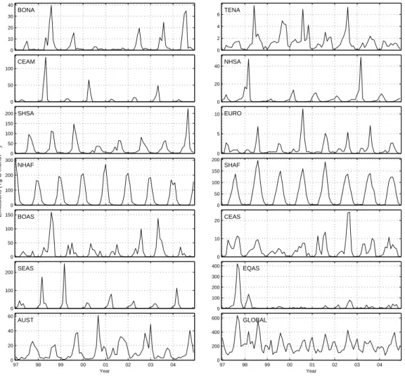
53 0 10 20 30 40 BONA 0 2 4 6 TENA 0 50 100 CEAM 0 20 40 NHSA 0 50 100 150 200 SHSA 0 5 10 EURO 0 100 200 300 NHAF Emissions (Tg C month −1 ) 0 50 100 150 200 SHAF 0 50 100 150 BOAS 0 10 20 CEAS 0 100 200 SEAS 0 100 200 300 400 EQAS 97 98 99 00 01 02 03 04 0 20 40 60 AUST Year 97 98 99 00 01 02 03 04 0 200 400 600 GLOBAL Year
Figure 8. Monthly fire emissions (Tg C month-1) for the regions defined in Fig. 1 and Table
1. Note that the seasonality in Africa during 1997-2000 was averaged from 2001-2004 (though the annual amplitude was allowed to vary).
Fig. 8. Monthly fire emissions (Tg C month−1)for the regions defined in Fig. 1 and Table 1. Note that the seasonality in Africa during 1997–2000 was averaged from 2001–2004 (though the annual amplitude was allowed to vary).
satellite-based measurements of CO in the northern hemi-sphere have previously noted the difference in seasonality between the two years (Edwards et al., 2004; Yurganov et al., 2005). Another region where the seasonality of emis-sions varied substantially was Central Asia; two peaks are visible in some years (1997, 2001, 2003) in Fig. 8, while in other years the first peak is less pronounced (1998, 2002). In Equatorial Asia, only in 1998 after the strong El Ni˜no, was substantial fire activity observed during February and March; usually the peak fire season occurred later in the year during the August–October period.
Studies using measurements of atmospheric CO from MO-PITT have identified a substantial mismatch in seasonal tim-ing of top-down (inverse) estimates of CO fluxes vs. bottom-up biogeochemical model estimates (P´etron et al., 2004; Arellano et al., 2006). In Fig. 9 we show results from Southern hemisphere Africa (SHAF) where the mismatch appeared largest. The MOPITT-derived approaches indicate that the peak fire season occurs in September; measurements
of Aerosol Optical Depth (MOD08 M3, available online at http://modis-atmos.gsfc.nasa.gov/) indicate a peak a month later, in October (Fig. 9a). In contrast, both the GBA2000 burned area product and our previous emission estimates that were based on VIRS fire counts (GFEDv1; van der Werf et al., 2004) peaked in June or July, up to 4 months ear-lier (Fig. 9b). Even though the peak fire season shifts to August in our approach described here using MODIS fire counts, there is still a 1–2 month offset with respect to the atmospheric-based approaches. There are several possible reasons for this continued offset. First, the fire season in SHAF shifts through time from west to east. When dividing SHAF at longitude 25◦E, the fraction of total SHAF burned area that is observed west of 25◦E is 48% for GBA2000, 46% for GFEDv1, and 41% for the burned area used in this study (Giglio et al., 2006). Greater burned area and emis-sions in the west causes the peak fire season for the entire region to advance to earlier times within the year. Another clue for the reasons behind this mismatch may come from
G. R. van der Werf et al.: Interannual variability in global biomass burning emissions 3433 54 J F M A M J J A S O N D 0 10 20 30 40 Petron et al (2004) Arellano et al (2006) MODIS AOD 0.6 0.5 0.4 0.3 0.2 Emissions (Tg CO month −1 ) AOD (−) J F M A M J J A S O N D 0 10 20 30 Month (year 2000) GFEDv2 emissions GFEDv1 emissions GBA2000 30 20 10 0 Emissions (Tg CO month −1 ) Burned area (10 4 km 2 month −1 )
Figure 9. Fire seasonality derived from different sources for southern hemisphere Africa (SHAF) for the year 2000. a) ‘top down’ derived seasonality using CO retrievals from the MOPITT sensor (Pétron et al., 2004; Arellano et al., 2006) and aerosol optical depth from MODIS. b) ‘bottom-up’ seasonality from this study (GFEDv2), our previous work (GFEDv1), and burned area from GBA2000 (Grégoire et al., 2002).
Fig. 9. Fire seasonality derived from different sources for south-ern hemisphere Africa (SHAF) for the year 2000. (a) “top down” derived seasonality using CO retrievals from the MOPITT sen-sor (P´etron et al., 2004; Arellano et al., 2006) and aerosol optical depth from MODIS. (b) “bottom-up” seasonality from this study (GFEDv2), our previous work (GFEDv1), and burned area from GBA2000 (Gr´egoire et al., 2002).
Table 5. Annual fire emissions of carbon, CO2, CO, and CH4in Tg year−1. Year carbon CO2 CO CH4 1997 2991 10 760 557 30 1998 3183 11 454 591 30 1999 2284 8291 392 19 2000 2038 7423 337 15 2001 2224 8108 365 17 2002 2386 8640 418 20 2003 2251 8143 397 19 2004 2320 8406 405 20 Average 2460 8903 433 21 SD1 403 1416 91 6 CV2 0.16 0.16 0.21 0.27 1Standard deviation. 2Coefficient of variation.
aerosol characteristics; late season aerosols have a higher albedo than aerosols in the beginning of the season (T. Eck, personal communication), which is likely to be the result of more burning in woodlands than in grasslands. Woodland fires emit larger amounts of CO per unit carbon burned than grassland fires, and this shift from grassland fires to wood-land fires may not be captured by our coarse resolution mod-eling framework. Modmod-eling at the MODIS native resolutions or even finer using other sensors may help in the future in identifying the role of these fine scale dynamics.
55
0 2 4 6x 10 4 Burned area (km 2 year −1) a) CIFFC This study
0 1 2
3x 10
5
Sukhinin et al. (04) This study
b) Burned area (km 2 year −1 ) 97 98 99 00 01 02 03 04 0 200 400 600
Kasischke et al. (05) This study
c) Year Emissions (Tg C year −1 )
Figure 10. Annual burned area for Canada (a) and Russia (b), and annual carbon emissions
for the boreal region (c). Results from this study were compared to a) burned area as
compiled by the Canadian Interagency Forest Fire Centre (CIFFC), b) burned area calculated
using AVHRR data by Sukhinin et al. (2004), and c) emissions from the “moderate severity
scenario” from Kasischke et al. (2005) using various sources of burned area combined with
the Boreal Wildland-Fire Emissions Model.
Fig. 10. Annual burned area for Canada (a) and Russia (b), and annual carbon emissions for the boreal region (c). Results from this study were compared to (a) burned area as compiled by the Canadian Interagency Forest Fire Centre (CIFFC), (b) burned area calculated using AVHRR data by Sukhinin et al. (2004), and (c) emissions from the “moderate severity scenario” from Kasischke et al. (2005) using various sources of burned area combined with the Boreal Wildland-Fire Emissions Model.
3.3 Burned area
The regions that burned most frequently during 1997– 2004 were northern hemisphere Africa, southern hemi-sphere Africa, and Australia (Tables 4 and 6). To-gether, these three savanna areas accounted for approxi-mately 80% of global burned area during our study pe-riod. The total burned area derived in this study for all of Africa is 2.4 million km2year−1in 2000, comparable to the 2.1 million km2year−1 as calculated using another
satellite-based approach (GBA2000, Gr´egoire et al., 2002). The dif-ference in total burned area in Australia is somewhat larger: approximately 0.7 million km2year−1as calculated here vs. approximately 0.5 million km2year−1by GBA2000.
Detecting burned area in tropical deforestation areas rep-resents a greater challenge, both because of consistent cloud cover and because of human manipulation of fire processes. Detailed burned area estimates associated with deforestation cannot be given, because of high heterogeneity within the 1◦×1◦ grid cells we have used here, and because pasture
56 0 2 4 6 8 0 500 1000 1500 2000 2500 3000 3500 c) BONA
Fuel consumption (kg C m −2 year −1)
0 2 4 6 8 0 1 2 3 4 5x 10 4 b)
CEAM, NHSA, and SHSA
Fuel consumption (kg C m −2 year −1) maintenance fires deforestation fires 0 2 4 6 8 0 2 4 6 8 10x 10 5 a)
NHAF and SHAF
Fuel consumption (kg C m −2 year −1)
Average annual burned area (km
2 year
−1
)
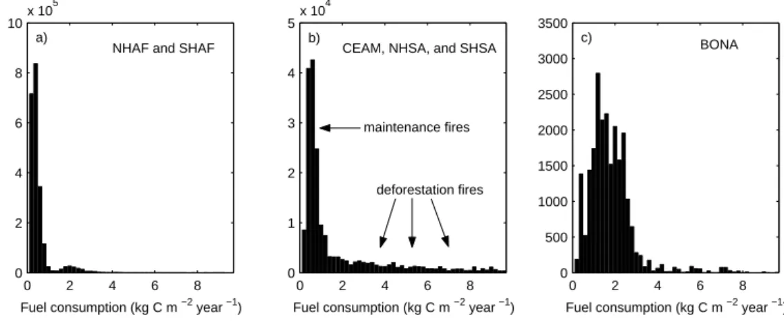
Figure 11. Frequency of occurrence of fuel consumption in different regions, a) Africa, b) Central America, Northern Hemisphere South America, and Southern Hemisphere South America, and c) boreal North America. Note the order of magnitude difference in vertical scale between the panels. Each bar represents a 0.2 kg C m-2 year-1 bin, centred upon its
mean.
Fig. 11. Frequency of occurrence of fuel consumption in different regions, (a) Africa, (b) Central America, Northern Hemisphere South America, and Southern Hemisphere South America, and (c) boreal North America. Note the order of magnitude difference in vertical scale between the panels. Each bar represents a 0.2 kg C m−2year−1bin, centred upon its mean.
Table 6. Area burned (×104km2year−1= Mha year−1)for different regions and years.
Region Year Average St.dev. St.dev./Average
1997 1998 1999 2000 2001 2002 2003 2004 BONA 1.5 4.9 2.3 0.7 0.4 2.6 2.3 4.0 2.3 1.5 0.66 TENA 0.9 1.7 2.6 2.3 1.4 1.7 1.5 1.2 1.7 0.5 0.34 CEAM 1.7 9.9 2.6 3.6 1.8 2.2 2.9 1.8 3.3 2.7 0.83 NHSA 3.4 5.2 1.6 4.5 4.4 3.6 4.8 3.8 3.9 1.1 0.29 SHSA 11.7 16.4 14.5 10.2 12.4 12.7 10.8 13.4 12.8 2.0 0.16 EURO 1.7 2.6 1.6 4.1 2.9 1.6 2.6 1.9 2.4 0.9 0.36 MIDE 0.1 0.1 0.3 0.2 0.6 0.5 0.4 0.4 0.3 0.2 0.54 NHAF 157.8 135.8 149.1 153.7 153.2 135.2 125.5 129.8 142.5 12.3 0.09 SHAF 65.1 97.8 72.8 76.5 84.0 82.4 79.6 75.3 79.2 9.6 0.12 BOAS 5.4 19.8 8.2 9.1 6.3 9.3 14.5 4.9 9.7 5.1 0.52 CEAS 21.1 15.7 8.6 12.8 16.5 26.7 17.1 18.9 17.2 5.4 0.31 SEAS 8.9 21.1 23.0 8.8 10.8 10.2 8.4 16.1 13.4 5.9 0.44 EQAS 16.7 5.3 1.1 0.8 0.8 3.4 1.4 2.9 4.0 5.3 1.32 AUST 41.5 36.0 52.9 70.7 78.7 58.9 24.8 44.9 51.0 18.0 0.35 Global 337.5 372.4 341.0 358.0 374.2 351.0 296.6 319.3 343.7 26.4 0.08
fires within these grid cells will dominate the burned area numbers.
In boreal regions, our burned area time series was corre-lated with independent estimates for Canada from the Cana-dian Interagency Forest Fire Centre (CIFFC) and for Russia (Sukhinin et al., 2004), but the magnitude differed in Russia (Fig. 10). This may be a consequence of the way we extended the MODIS burned area time series back in time using ATSR fire counts. Since ATSR only detects fires at night and fire activity peaks during daytime, ATSR may more easily detect large fires that burn for longer periods. This is a potential rea-son for the higher burned area in the high fire year of 1998 in boreal Asia than reported by Sukhinin et al. (2004). This was
not observed in Canada, where our burned area was similar to independently derived estimates.
3.4 Fuel consumption
Combustion completeness (CC) and fuel loads were in-versely related; in general the higher the fuel loads, the lower CC (Table 4). This was because high fuel loads were often a result of an increased abundance of stem and coarse woody biomass that tend to combust incompletely (Table 3). Boreal regions and Equatorial Asia did not follow this trend; here organic soil carbon and peat represented a large fraction of the fuel load (Table 4). In boreal regions, biomass and litter
pools were equally large, but a larger part of the emissions stemmed from the combustion of litter because of the higher CC observed for these fuels. CC was also high in deforesta-tion regions (SHSA, for example) because we increased CC for stems and coarse woody debris when there were high lev-els of fire persistence to represent repeated human aggrega-tion and burning of fuels.
The highest fuel loads (∼10 kg C m−2)were predicted to occur in Equatorial Asia, because of high aboveground fuel loads and peats in wetland areas. Other tropical areas where fires were being used to clear forests also had high fuel loads within burned areas, including Central and South America. In both boreal North America and boreal Asia, fuel loads were approximately 3.5 kg C m−2, and were almost evenly distributed between aboveground biomass and litter fuels. In savanna regions, fuel loads were highest in southern hemi-sphere Africa (1.3 kg C m−2)because a substantial part of
the burning occurred in woodland areas, and were lowest in Australia (0.4 kg C m−2)where much of the burning oc-curred in low productivity grasslands. Fuel loads in northern hemisphere Africa (0.7 kg C m−2)fell in between these two regions.
In frequently burning savannas, there was a clear upper limit on fuel consumption. Most savannas that burned an-nually were the more productive savannas with NPP val-ues of approximately 1000 g C m−2year−1 (van der Werf et al., 2003). Since half of the NPP was allocated below-ground and was not accessible for fires, fuel loads in an-nual burning savannas were at most 500 g C m−2. How-ever, not all above ground biomass was available for fires since microbes, herbivores, and humans also consume the available carbon. In addition to this upper threshold, there was also a lower threshold of approximately 100 g C m−2
that may represent the minimum levels of fuel necessary to sustain fire spread (van Wilgen and Scholes, 1997). We found that the majority of the fires in Africa consumed be-tween 200 and 400 g C m−2year−1 (Fig. 11a), which is on the high end of most remote sensing and modeling stud-ies (Scholes et al., 1996; Barbosa et al., 1999; H´ely et al., 2003). In tropical America (CEAM, NHSA, SHSA) there was a clear distinction between pasture maintenance and sa-vanna fires that accounted for much of the burned area but consumed little fuel, and deforestation fires with much larger fuel consumption but lower burned area (Fig. 11b). Pas-ture maintenance fires occur in managed grasslands and are ignited on purpose, mainly to prevent trees from invading the landscape and for nutrient recycling (Fearnside, 1990). In Africa, there were fewer fires with high fuel consump-tion (>3 kg C m−2year−1), providing evidence for less fire-driven deforestation than in South America. Fuels consumed in the boreal ecosystems consisted primarily of litter and soil carbon (Table 4). In boreal North America, the majority of the fires consumed between 1 and 2.5 kg C m−2year−1, with a mean of 1.9 kg C m−2year−1, stemming largely from com-bustion of the duff layer and organic soil carbon, and with
57 97 98 99 00 01 02 03 04 1100 1200 1300 PPT (mm year −1 ) PPT TEMP Air temperature ( o C) a) 97 98 99 00 01 02 03 04 17 17.5 18 97 98 99 00 01 02 03 04 2000 2500 3000 3500 4000 Emissions (Tg C year −1 )
BB SOI SOI index
b) 97 98 99 00 01 02 03 04 −20 −10 0 10 20 97 98 99 00 01 02 03 04 −1000 0 1000 Anomaly (Tg C year −1 ) NPP Rh BB c) 97 98 99 00 01 02 03 04 −1000 0 1000 Anomaly (Tg C year −1) Year NEP NBP d)
Figure 12. Annual values of: a) NPP weighted precipitation (PPT) and air temperature (TEMP), b) biomass burning (BB) emissions and Southern Oscillation Index (SOI,
http://www.bom.gov.au/climate/current/soihtm1.shtml, c) NPP, Rh, and biomass burning
emission anomalies, and c) net ecosystem production anomaly (NEP) and net biome production anomaly (NBP). Global fire emissions were negatively correlated with the SOI (r = -0.53).
Fig. 12. Annual values of: (a) NPP-weighted precipitation (PPT) and air temperature (TEMP), (b) biomass burning (BB) emis-sions and Southern Oscillation Index (SOI, http://www.bom.gov. au/climate/current/soihtm1.shtml, (c) NPP, Rh, and biomass
burn-ing emission anomalies, and (d) net ecosystem production anomaly (NEP) and net biome production anomaly (NBP). Global fire emis-sions were negatively correlated with the SOI (r=−0.53).
minor contributions from stems and leaves (Fig. 11c). This distribution is similar to the modeled distribution reported by Amiro et al. (2001).
3.5 Emissions
Average annual emissions over the 8 year time period were 2.5 Pg C year−1 (Tables 5 and 7, Fig. 12b). African
emis-sions accounted for 49% of the total and southern hemi-sphere South America contributed another 13%. Other major contributors included Equatorial Asia (11%), boreal regions (9%), Southeast Asia (6%), and Australia (6%).
Over the 8 year period, there was significant IAV, espe-cially during the first 4 years (Fig. 12b). Emissions in both 1997 and 1998 were approximately 1 Pg C year−1 higher than in 2000. In contrast, global PPT was low in the second half of 1997 and in 1998 and at a maximum in 2000 (Adler
Table 7. Fire emissions for different regions and years (Tg C year−1).
Region Year Average St.dev. St.dev./Average
1997 1998 1999 2000 2001 2002 2003 2004 BONA 16 93 37 11 7 45 55 90 44 34 0.76 TENA 8 19 25 24 14 20 12 10 16 6 0.39 CEAM 15 212 25 98 20 31 81 17 62 68 1.10 NHSA 32 83 11 29 38 27 80 33 42 26 0.62 SHSA 272 314 360 160 241 264 216 443 284 88 0.31 EURO 9 14 8 25 14 13 15 10 14 5 0.39 MIDE 0 0 1 0 1 1 1 1 1 0 0.46 NHAF 740 565 606 665 720 615 541 562 627 75 0.12 SHAF 465 721 535 567 606 568 581 565 576 72 0.12 BOAS 71 438 134 140 107 221 330 66 188 133 0.71 CEAS 60 45 26 37 49 72 45 45 47 14 0.29 SEAS 102 265 314 73 159 97 77 182 159 90 0.57 EQAS 1089 317 66 51 50 257 86 170 261 349 1.34 AUST 111 96 136 157 199 156 131 127 139 32 0.23 Global 2991 3183 2284 2038 2224 2386 2251 2320 2460 403 0.16
et al., 2003, Fig. 12a). 1997 was a high fire year because of emissions in equatorial Asia, largely stemming from the combustion of peat in Indonesia (Page et al., 2002). 1998 was a high fire year because of increased burning across multiple continents, including equatorial Asia, boreal North America and Asia, and Central and South America. Only in north-ern hemisphere Africa and Australia were emissions below average (Table 7). During the final 4 years of the study pe-riod, the range of emissions was lower, but emissions were elevated from 2000.
By far the region with the largest IAV was equatorial Asia, both in absolute and in relative terms, with a standard devi-ation that was approximately 1.3 times larger than the aver-age (Table 7). Emissions in 1997 were over 20 times higher than in the year 2000, indicating a strong dependence on lo-cal climate and/or human activity. Emissions in equatorial Asia were elevated again in 2002. More detailed inversion studies using MOPITT should further constrain the magni-tude of these 2002 anomalies, and their impact on high CO2
growth rates observed during 2002 and 2003. Other regions with substantial IAV include boreal North America and Asia, Central America, and northern hemisphere South America. IAV in frequently burning Africa was low.
Most savanna and grassland fires occurred in Africa and Australia. Average annual emissions from Africa were 1203 Tg C year−1, and emissions from northern hemisphere Africa (627 Tg C year−1)were somewhat higher than emis-sions from southern hemisphere Africa (576 Tg C year−1). Average fuel consumption on the other hand, was higher in southern hemisphere Africa largely because relatively more fires were detected in woodlands, whereas almost all the fires in northern hemisphere Africa occurred in grasslands with
lower percentages of woody vegetation. Other studies have reported lower emissions (Scholes et al., 1996; Barbosa et al., 1999; Hoelzemann et al., 2004), but relatively higher IAV (Barbosa et al., 1999). Some of this difference can probably be attributed to higher fuel loads in our study as our burned area estimates are comparable or even lower than those re-ported in previous studies. Emissions calculated by Ito and Penner (2004) are comparable to our estimates, with a dif-ference of about 10%, depending on the scenario used by Ito and Penner (2004).
3.6 Net biome productivity
Average annual global NPP was 58 Pg C year−1. Annual NPP and Rhvalues were approximately 23 times larger than fire fluxes (58 vs. 2.5 Pg C year−1). As a consequence, rela-tively small variations in the balance between NPP and Rh can have a large effect on IAV of net biome productivity (NBP) and the CO2 growth rate. NPP was highest in 2000
and lowest in 1998, with a difference of 1.8 Pg C year−1 (Fig. 12c). About 95% of NPP was returned to the atmo-sphere via Rh during 1997–2004. Variability of Rh be-tween years was similar to NPP, but with a smaller ampli-tude. The highest levels of Rh were observed in 2000, and lowest in 1998 and 2002, with a difference of approximately 1.0 Pg C year−1.
Because NPP and Rh tended to vary in parallel in CASA, the global net ecosystem production (NEP, NPP – Rh)was smaller than the anomalies in NPP. Large net uptake occurred in 1997, 2000, and 2004, while carbon was released during 1998 because the negative NPP anomaly was larger than the Rh anomaly. In 2003 modelled variations in NPP and Rh
were somewhat different from other years; Rhshowed only a small negative anomaly while NPP was inhibited much more, leading to a source (Fig. 12c). The NEP signal was amplified by IAV in fires. The net result was that net biome production (NBP = NEP – fire emissions) had a larger amplitude than NEP. This was most evident during the first 5 years of the study period.
3.7 Differences with earlier estimates
Emission estimates from our earlier studies were released in 2004 as the “Global Fire Emissions Database” (GFED ver-sion 1), covering the 1997–2001 period. These estimates were compared to results from, or used as a priori infor-mation in, several inversion studies (Arellano et al., 2004; P´etron et al., 2004; van der Werf et al., 2004). The main limi-tations of GFEDv1 as indicated by inversion studies were the underestimation of emissions anomalies in Equatorial Asia, Central and northern South America, and in the boreal re-gions. Inversion analyses suggest that GFEDv1 overesti-mated the magnitude of southern Africa emissions and that the seasonal phasing of emission in this region was off by several months.
Discrepancies between the inversion studies and our bottom-up results may help to identify regions where the bottom-up approach has a problem representing biomass burning processes, assuming that the emission factors that translate the carbon emissions into the CO fluxes used in these inversions are correct (and that inversion don’t suffer from other types of biases). One example is the combustion of peat that was not taken into account in GFEDv1, and may have been partly responsible for the underestimation of emis-sions from equatorial Asia.
There are numerous differences between the results pre-sented here and those previously reported in GFEDv1, mainly stemming from the use of improved burned area and the inclusion of organic soil carbon and peat burning. For GFEDv1 we used a single global relationship between fire counts, fraction tree cover, and burned area. Here, many more MODIS scenes with burned area were available for fire count calibration (446), allowing us to use regionally-based fire count to burned area relationships that depended on fire count cluster size and fire persistence, in addition to fractional tree cover (Giglio et al., 2006). This has led to a decrease of Southern African emissions because of lower burned area. The inclusion of organic soil carbon and peat burning increased emissions in boreal regions and in equa-torial Asia. Another difference is that we formerly had a broad band of relatively low emissions around the main de-forestation areas in South America and Indonesia, our new results indicate that the emissions are higher in a smaller band known to have high rates of clearing (e.g., Mato Grosso, southern and eastern Kalimantan). However, total emissions in Central and Southern America are lower in our current in-ventory, and diverge from results obtained from inverse
stud-ies (that suggested our previous dataset underestimated emis-sions in these regions; Arellano et al., 2006).
3.8 Uncertainties 3.8.1 Burned area
Burned area estimates have only recently become available from different satellite sensors, allowing for a comparison of different approaches. In boreal and tropical savanna ecosys-tems, independent estimates of burned area are converging, for large regions within 20%, although interannual differ-ences can be larger. Obviously this does not rule out the possibility that independent products can suffer from iden-tical biases, but it does provide some optimism compared to earlier estimates that differed by over a factor 2 (Kasischke and Penner, 2004).
In deforestation regions, burned area estimates remain poorly constrained. There are several reasons for this, the most important being consistent cloud cover and mechanized aggregation of fuels into piles that make burned area detec-tion problematic. The approach of Giglio et al. (2006) de-tects more burned area in areas undergoing active deforesta-tion than other published estimates (Gr´egoire et al., 2002; Simon et al., 2004), but it remains unclear how to assess un-certainty levels associated with this product. With greater use of high resolution satellite data it the future, it is likely that burned area estimates will increase, especially in closed-canopy tropical forest ecosystems (Silva et al., 2005).
Because we used a statistical approach to estimate burned area from fire counts (Giglio et al., 2006), burned area esti-mates were available only for coarse resolution grid cells. This may introduce a bias when fire processes show spa-tial heterogeneity. Future studies of global biomass burning emissions will profit from comparisons with studies that use burned area at finer resolution, ideally employing methods to scale up from fine to coarse resolutions.
3.8.2 Fuel loads
As burned area estimates improve from higher resolution satellite data and refined algorithms, uncertainties in fuel loads may become the limiting factor in estimating emis-sions (French et al., 2004; Hoelzemann et al., 2004). Al-though using satellite data has improved estimates of spatial and temporal variability in fuel loads, approaches for cali-brating these estimates using measured values are still in their infancy. Reasons for this include a mismatch in scale be-tween the measurements at plot level and the much coarser model grid cell, and a lack of data. Calibrating against satellite-based measurements of, for example, biomass es-timates based on satellite measured vegetation height are likely to contribute to decreasing uncertainties. Following Amiro et al. (2001) and H´ely et al. (2003), we have pre-sented histograms of carbon consumption (Fig. 11). These