Decomposing a Graph into Shortest Paths with Bounded Eccentricity

HAL Id: hal-01511357

https://hal.archives-ouvertes.fr/hal-01511357v2

Preprint submitted on 14 Sep 2017

HAL is a multi-disciplinary open access

archive for the deposit and dissemination of

sci-entific research documents, whether they are

pub-lished or not. The documents may come from

teaching and research institutions in France or

abroad, or from public or private research centers.

L’archive ouverte pluridisciplinaire HAL, est

destinée au dépôt et à la diffusion de documents

scientifiques de niveau recherche, publiés ou non,

émanant des établissements d’enseignement et de

recherche français ou étrangers, des laboratoires

publics ou privés.

Bounded Eccentricity

Etienne Birmelé, Fabien de Montgolfier, Léo Planche, Laurent Viennot

To cite this version:

Etienne Birmelé, Fabien de Montgolfier, Léo Planche, Laurent Viennot. Decomposing a Graph into

Shortest Paths with Bounded Eccentricity. 2017. �hal-01511357v2�

Bounded Eccentricity

Etienne Birmelé

, Fabien de Montgolfier

, Léo Planche

, and

Laurent Viennot

1 MAP5, UMR CNRS 8145, Univ. Sorbonne Paris Cité 2 IRIF, UMR CNRS 8243, Univ. Sorbonne Paris Cité 3 Inria

Abstract

We introduce the problem of hub-laminar decomposition which generalizes the one of computing a shortest path with minimum eccentricity (MESP). Intuitively, it consists in decomposing a graph into several paths that collectively have small eccentricity and meet only near their extremities. The problem is related to computing an isometric cycle with minimum eccentricity (MEIC). It is also linked to DNA reconstitution in the context of metagenomics in biology. We show that a graph having such a decomposition with long enough paths can be decomposed in polynomial time with approximated guaranties on the parameters of the decomposition. Moreover, such a decomposition with few paths allows to compute a compact representation of distances with additive distortion. We also show that having an isometric cycle with small eccentricity is related to the possibility of embedding the graph in a cycle with low distortion.

1998 ACM Subject Classification G.2.2 Graph Theory

Keywords and phrases Graph Decomposition, Graph Clustering, Distance Labeling, BFS, MESP

1

Introduction

The goal of this paper is to extend the MESP (Minimum Eccentricity Shortest Path) Problem from Dragan and Leitert [5] and the related problem of recognizing k-laminar graphs from Völkel et al. [16]. Both consist in finding a shortest path (in the sense that no path joining the same endpoints is shorter) k-dominating a graph (every vertex is at distance at most k from that path). The k-laminar problem additionally requires that path to be a diameter (there is no longer shortest path in the graph). Relationships between the two parameters

are derived in [4].

To generalize this problem to more complex underlying structures, we introduce the problem of decomposing a graph into subgraphs with bounded shortest-path eccentricity. More precisely, we introduce the hub-laminar decomposition as a set of paths that k-dominates the graph and meet only near their extremities. To formalize this property, we introduce the notion of hub, that is a ball with fixed radius r centered at a path endpoint. The laminar associated to a path is the set of nodes k-dominated by the path. Our definition requires that an edge between two nodes belonging to two different laminars must also belong to a hub. The degree of a hub is then the number of laminars that meet in the hub. The main result of the paper is that computing such a decomposition becomes tractable when hub centers are far enough one from another, or equivalently when paths are long enough. The MESP problem is equivalent to a hub-laminar decomposition with one laminar.

Such a generalization is naturally interesting in networks where one might want to identify a set of speedy linear routes that are “highly accessible” with applications in communication networks, transportation planning and water resource management. It is also motivated by

DNA assembly in biology. DNA sequencing proceed through the reading of DNA fragments that must be assembled. When a single DNA strand is sequenced, comparison of fragments leads to a graph with “laminar” structure [16] that is with large diameter and small shortest path eccentricity. In the context of metagenomics, several DNA strands are sequenced together and more complex structures appear (see Figure 1 in [16]). Identifying the laminar structures of such graphs is typically encountered in metagenomic approaches for evolution questions (see e.g. [13]). The problem of the assembly (gluing DNA fragments to reconstruct a DNA strand) is then mixed with that of binning (sort DNA strands into groups that represent an individual genome or genomes from closely related organisms). See [14] for a presentation of assembly and binning problems in the context of metagenomics. Efficient decomposition of a graph into laminars could thus enhance the techniques for assembly and binning in this context.

The problem of decomposing a graph into λ laminars that k-cover the graph is not well defined as there may be several trade-offs of parameters λ and k. However, we show that when laminars are long enough compared to parameters r and k, then all (r, k)-hub-laminar decompositions are equivalent (same global structure) and have closely located hubs (except for hubs of degree two that do not affect the global structure). This implies for example that the positions of the extremities of the minimum eccentricity shortest path (MESP) can be approximated within O(k) distance when the diameter of a graph is large with respect to the eccentricity k of the MESP.

From a graph perspective, a very natural generalization of MESP is the problem of finding a minimum eccentricity isometric cycle (MEIC), that is a cycle preserving distances that has minimum eccentricity k. Note that such a cycle can be seen as a hub-laminar decomposition with two laminars and two hubs with degree two. An important motivation for the MESP problem is its relationship with embedding a graph into the line with small multiplicative distortion [5]. We similarly show that the MEIC problem is related to embedding a graph into a circle with low multiplicative distortion, i.e. such that distances in the circle are within a constant factor of distances in the graph. Note that circle distortion is bounded by line distortion as a line segment can isometrically be embedded in a sufficiently long circle. (However, line distortion can be much larger than circle distortion.) Graph embedding in

classical metrics is a well studied problem [9, 10]. Another related subject with abundant literature is that of compactly representing the distances of a graph [15, 12]. We show that a decomposition with few laminars ensures a compact representation of distances with bounded additive distortion.

Related works:

Finding a MESP is NP-complete but can be approximated within a constant factor [5]. Better trade-off between computation time and approximation factor for MESP is obtained in [4]. The problem of efficiently representing the distances in a graph encompasses a vast literature dating from metric embedding [1]. Approximating embedding with low distortion is introduced in [2] where some results are provided in the case of the line. The case of embedding the metric induced by an unweighted graph is studied in [3]. Embedding a graph metric into the line with minimum distortion is NP-complete but fixed parameter tractable with respect to distortion [6]. Approximate distance oracles, i.e. compact data-structures for representing an approximation of distances, are investigated in [15]. A particular approach introduced by Peleg [12] resides in assigning a label to each node of a graph such that the distance between two nodes can be estimated from their labels. Several result exist about the trade-off between label size and approximation quality. Exact distance estimation is

investigated in [8] and requires Ω(n) bits labels for general graphs. Approximation with a constant factor and sub-linear label size is derived in [15]. Some results concern additive approximation such as [7] in the case of hyperbolic graphs. A longest isometric cycle can be found in polynomial time [11].

2

Definitions

We consider finite, undirected and connected graphs (the connectivity is always assumed within the paper). Given a graph G, with vertex set V (G) and edge set E(G), we let dG(u, v)

denote the distance between two vertices, i.e. the length of a shortest path from u to v. When the graph G is clear from the context, we omit the G subscript and simply write d(u, v). Let B(u, r) = {v ∈ V (G) | d(u, v) ≤ r} denote the ball of radius r centered at u. Given a set of vertices U we set B(U, r) = ∪u∈UB(u, r). Given two sets U and W of vertices, we say

that U k-covers W when every vertex in W is at distance at most k from some vertex in

U , i.e. W ⊆ B(U, k). We say that U has eccentricity k, denoted ecc(U ) = k, when k is the

smallest integer such that B(U, k) = V (G). A path P in G is a sequence of nodes such that any two consecutive nodes are linked by an edge of G. We consider only simple paths: a node appears at most once in the sequence. The first node of the sequence and the last one are called the endpoints of P . For the simplicity of notations, we also let P denote the set of nodes appearing in the sequence. For any vertices u and v on P , we denote by Puv the

subpath of P having u and v as endpoints.

2.1

Hub-laminar decomposition

IDefinition 1 (Hub-laminar decomposition). Consider a connected undirected graph G, two positive integers r and k, H = {h1, . . . , hq} a set of vertices of G called hub centers, and

P = {P1, . . . , Pp} a set of paths of G called laminar paths. A ball B(h, r) with r ∈ H is called

a hub, and a set B(P, k) with P ∈ P is called a laminar. (H, P) is an (r, k)-hub-laminar

decomposition of G if the following conditions are satisfied:

1. each laminar links two hubs centers: the endpoints h, h0 of any P ∈ P belong to H and for every other hub h00∈ H \ {h, h0_{}, B(P, k) ∩ B(h}00_{, r + 1) = ∅ ,}

2. the laminars and the hubs cover G: V (G) ⊆S

h∈HB(h, r) ∪

S

P ∈PB(P, k),

3. each laminar path is locally a shortest path: any path P ∈ P with endpoints h and h0 is a shortest path of the graph G[B(P, k) ∪ B(h, r) ∪ B(h0, r)],

4. laminars meet at hubs only: for all i 6= j and uv ∈ E(G) such that u ∈ B(Pi, k) and

v ∈ B(Pj, k), there is a hub center h ∈ H such that Pi and Pj both have h as endpoint

and u, v ∈ B(h, r).

The minimal laminar length of a decomposition (H, P), denoted l, is the minimal length of the paths in P. Its laminar size, denoted λ, is the number of paths in P.

A hub-laminar decomposition (H, P) with l ≥ 2r + 1 forms a partition of the edges of G in the following sense: each edge is either inside exactly one hub (possibly touching many laminars ending in that hub), i.e ∃!h ∈ H s.t. u, v ∈ B(h, r); or, else, inside a unique laminar (possibly touching one hub extremity of that laminar), i.e, ∃!P ∈ P s.t. u, v ∈ B(P, k).

Figure 1 illustrates this definition and the notion of quotient graph that we define next. This definition basically defines a decomposition into k-neighborhoods of internally far apart shortest paths. It may seem a bit involved, but we think it expresses in a minimalist way what we mean by “internally far apart” with Item 4. Items 1 and 2 indicate that the graph is decomposed into laminars which are k-neighborhoods of certain paths and hubs which

Graph G

r k

Quotient graph of G

Reduced quotient graph of G

Figure 1 Illustration of an hub-laminar decomposition with r = 2, k = 1. Every vertex is at

distance r from a hub center (diamond vertices) or at distance k from a laminar path (bold paths between hub centers).

are balls centered at the extremities of those paths. Item 3 requires path to be shortest in the induced graph, and not in G, to allow laminars with different length (otherwise, a long laminar between two hubs could be shortcut by one or more laminars forming a paths between these hubs).

2.2

Quotient graph and equivalence between decompositions

As previously mentioned, the hub-laminar decomposition gives naturally raise to a skeleton, which can be simplified into a quotient graph.

IDefinition 2 (quotient graph and reduced quotient). Given a graph G and an (r, k)-hub-laminar decomposition (H, P) of G, the quotient of this decomposition is an edge-labeled multigraph with vertex-set H and for each P ∈ P with endpoints h, h0 there is an edge hh0 whose label is the length of P .

The degree of a hub denotes the degree of the corresponding vertex in the quotient graph, or equivalently the number of laminar paths its center is the endpoint of.

The reduced quotient graph of a decomposition (H, P) is the multigraph obtained from its quotient graph by repeatedly removing degree 2 nodes: for every vertex u of the quotient incident with exactly two edges uv and uw with respective labels a and b, u and both edges are removed and a new edge vw is added with label a + b. (It is a loop when v = w.)

When the quotient is not a cycle (a case specifically adressed by MEIC, see Section 3) the reduced quotient is well defined and unique (recall graphs are supposed connected).

IDefinition 3 (equivalence between decompositions). Two hub-laminar decomposition of a same graph G, possibly with different parameters r, k, are D-equivalent if they have the same reduced quotient graph, up to an isomorphism φ of vertex-sets such that d(h, φ(h)) ≤ D (d is the distance between hub centers in G, not in the reduced quotient)

2.3

Isometric cycle, circle embedding and distance labeling

A cycle C in a graph G is isometric if it preserves distances, i.e. dC(u, v) = dG(u, v) for all

u, v ∈ V (C). In other words, for any pair u, v of nodes on the cycle, one of the two path

linking u and v in the cycle is a shortest path in the graph. Note that an isometric cycle is necessarily an induced cycle. The MEIC problem consists in finding an isometric cycle with minimum eccentricity. It can be shown to be NP-complete following a similar proof as [5] for the NP-completeness of MESP problem.

A circle embedding of a graph G is a mapping f : V (G) → C where C is a circle of given length c. It has distortion γ if dG(u, v) ≤ dC(f (u), f (v)) ≤ γdG(u, v) for all u, v in V (G).

The circle distortion cd(G) of G is the minimum distortion of a circle embedding of G. A distance labeling of a graph G consists in assigning a label Luto each node u ∈ V (G)

together with a distance estimation function f that outputs an estimation of dG(u, v) when

given Luand Lvas input. It has additive distortion α if dG(u, v) ≤ f (Lu, Lv) ≤ dG(u, v) + α

for all u, v in G.

3

Main results

Obviously, the reduced quotient graph of a graph having a (r, k)-hub-laminar decomposition follows the following trichotomy: it is either a path, a cycle or has a degree three node. We treat separately the three cases.

In the first case, the graph has a shortest path with eccentricity max {3k, 2r} and can be recognized through an approximate MESP algorithm such as [4]. (The max {3k, 2r} bound is a consequence of Lemma 12 given in Section 4.) In the second case, the graph has an isometric cycle with eccentricity at most max {3k, 2r}. To recognize such graphs, we propose an approximate MEIC algorithm:

ITheorem 4. Given a graph containing a K-dominating isometric cycle with length `, a 6K-dominating isometric cycle can be computed in O(n4.752_{log(n)) time. Moreover, the}

computed cycle is indeed 3K-dominating when ` ≥ 12K + 2.

We obtain therefore an algorithm for approximating circle embedding with low distortion.

ICorollary 5. If a graph has circle distortion γ, it is possible to embed it in a circle with

distortion O(γ2_{) in polynomial time.}

Recognizing the general case of decomposition is not a well defined problem as several decompositions may yield different trade-offs of the parameters. However, when laminars are long enough, all (r, k)-hub-laminar decompositions are indeed O(k) equivalent. This can be seen as a consequence of the following recognition result.

ITheorem 6. Given a graph G having a (r, k)-hub-laminar decomposition (H, P) of minimal

laminar length ` ≥ 8r + 60k + 4 and integers K, R such that K ≥ 3k, R ≥ 2K + 3r + 3k and

2R + 8K < ` − 2r − 18k − 4, it is possible to compute in O(min(n, λ)m) time a (K,

R)-hub-laminar decomposition which is (K + 2r)-equivalent to (H, P).

From the graph metric point of view, we obtain then a compact representation of distances:

ICorollary 7. Given a graph G having an (r, k)-hub-laminar decomposition with laminar

size λ, it is possible to compute in polynomial time a O(max {k, r})-additive distance labeling with O(λ log n) bit labels.

Due to lack of space, the proofs of these theorems, and of the lemmas and propositions stated below, are put in Appendix.

4

Algorithms

4.1

Minimum Eccentricity Isometric Cycle

We propose to approximate the MEIC problem by computing a longest isometric cycle, that is an isometric cycle of G with maximum length. The following lemma shows that a longest isometric cycle O(k)-dominates any k-dominating isometric cycle.

ILemma 8. Let G be a graph with an isometric cycle C = c1, ...cp k-dominating G, and

let D be a longest isometric cycle of G. Every vertex of C is at distance at most 5k of D. Furthermore, if D has length more than 12k + 2 then every vertex of C is at distance at most

2k of D.

Consequently, a longest isometric cycle in a graph is a 6-approximation for the MEIC problem, and a 3-approximation when the graph has a diameter large enough. As shown in [11], a longest isometric cycle can be computed in O(n4.752_{log(n)) time. Theorem 4 is thus a} direct consequence of this and Lemma 8.

4.2

General case outline

Consider a graph G having a (r, k) hub-laminar decomposition (H, P) of minimal laminar length ` and having at least one hub of degree at least 3. The underlying idea of the algorithm is to use BFS (Breadth-first search) to compute shortest paths and their K-neighborhoods,

K being chosen large enough to dominate every laminar traversed by the considered shortest

paths, but small enough compared to ` to detect all hubs of degree at least 3.

The first step, called F indHubs, consists in applying the procedure N extHub described in section 4.4 until it discovers no new hubs. This step yields two sets of hub-centers A and

B, respectively called unmovable and movable hub-centers, which will be used to determine

the laminars. A unmovable hub center a ∈ A means we a sure there exists exactly one hub center h ∈ H such that d(a, h) is bounded. It will be shown that A contains exactly one such vertex for every hub-center of H which degree is not 2.

A movable hub center b ∈ B will only be added by N extHub in a configuration corres-ponding to a cycle in the quotient graph of (H, P) containing only one hub of degree at least 3, like the three laminars on the left of Figure1. This is called a Problematic Configuration We know there exists at least Degree 2 hub h ∈ H somewhere in that cycle, but if they are thin enough they may remain merged in the laminars and we can not bound d(b, h), and in the second step b may be moved.

The laminars are determined in a second step by the F indLaminars procedure, which links the hub-centers of the previous step by shortest paths. The only difficulty which has to be taken into account refers to hubs of degree 2 in (H, P). Indeed, the BFS runs of the hub-detection step may have missed one of them because they K-dominated it, whereas the BFSs of second step don’t. In that case, the set of hubs A is adapted by adding the new discovered hub, and if needed, the corresponding movable hub center is deleted from B.

Figure gives a summary of the two steps by showing a possible outcome of the F indHubs and F indLaminars on an example. The F indHubs procedure detects all hubs of degree different from 2 and some of those of degree 2. Moreover, it places a movable hub on each problematic configuration. F indLaminars then computes the corresponding laminars, adding new hubs if a hub of degree 2 missed in the first step is detected. Some of them may however still be undetected, being replaced by a movable hub or just missing in the final decomposition. The quotient graphs of the decomposition supposed by Theorem 6 and of the constructed decompositions may therefore be different, but their reduced quotients are equal.

4.3

Some rules to compute a decomposition

We rely on the following properties for running our algorithm. The first tool is used to identify hub centers. Fortunately there is a pattern that, when it occurs, signals that any hub-laminar decomposition must have a hub nearby:

Unknow decomposition Hubs computed with FindHubs

a1

a2 a3 a4

a5

b1

Decomposition after FindLaminars a1

a2 a3 a4

a5

a6

Figure 2 Illustration of the different steps of the algorithm. The (H, P) decomposition is unknown

(top left). Notice a Problematic Case on the right of the graph: a cycle of laminar with only one degree not 2 hub. First, hub centers are computed such that every degree not 2 hub B(h, r), h ∈ H is covered by B(ai, R), ai∈ A (top right). Finally the laminar are computed (greyed, bottom) and

some movable hubs may be moved (like b1 moved into a5). Some thin degree 2 hubs from H are

not found but merged in the K-laminars. Fortunately the hub center a5 was found by BFS in the

second step, but we could also have output b1 instead, or both a5 and b1, yielding in any case an

equivalent reduced quotient.

ILemma 9 (Hub trigger). Consider three numbers r, k and K ≥ 3k. If there exists

a shortest path Q from a to b

a vertex u ∈ V (Q) such that d(a, u) > K + 6k and d(b, u) > K + 6k a vertex v such that d(u, v) = K

a vertex w such that vw ∈ E(G) and d(Q, w) = K + 1 and d(u, w) = K + 1,

then any (r, k)-hub-laminar decomposition (H, P) has a hub center h ∈ H with d(u, h) ≤ K +r.

Fig. 3 (right) illustrates this. This pattern, when found, allows to propose u as an hub. And it is very powerful, since every hub h of degree at least three of any (r, k)-hub-laminar decomposition shall trigger this pattern, for any shortest path Q passing close to h and long enough, as the following lemma says:

ILemma 10 (Degree ≥ 3 Hub Detection). If a graph admits an (r, k)-hub-laminar

decom-position (H, P), and has a hub h ∈ H whose degree is at least 3, then for any K ≥ 3k

shortest path Q from a to b

vertex u ∈ V (Q) such that d(a, u) > r + 4K + 9k + 2 and d(b, u) > r + 4K + 9k + 2 and d(u, h) ≤ K

there exists

a vertex x ∈ V (Q) such that d(a, x) > K + 6k and d(b, x) > K + 6k a vertex v such that d(x, v) = K

a vertex w such that vw ∈ E(G) and d(Q, w) = K + 1 and d(x, w) = K + 1,

Notice that if a graph admits an (r, k)-hub-laminar decomposition (H, P) where all hubs have degree at least three, then the pattern is enough to find all its hubs, or more exactly to compute a set of hubs H0 which is in bijection φ with H, i.e. for all h ∈ H d(h, φ(h)) ≤ K + r.

h h0 v0 u0 _v u (a) Q P (b) h u v w Q (c) h1 h2 hz d f K ≤ R

Figure 3 Illustration of the structural properties. (a) Lemma 12: The part of the laminar

k-covered by Pu0_v0 is K-covered by Q. (b) Lemma 9: If Q goes through a hub of degree ≥ 3, a triplet

u, v, w can be found, and it is the only such case far apart the extremities of Q. (c) Lemma 11.

Of course to do so in polynomial time we shall use a clever collection of paths Q to trigger all hubs. This is the idea developed in the algorithm. But before we shall explain how to deal with degree 1 hubs, the “dead end” hubs.

ILemma 11 (Hub in the dead-end). Consider the graph G0 _{induced by a sequence of incident}

hubs and laminar H1, L1, H2, ...Hz, such that h1 and hz are at distant of at least 2R + r + 2.

Suppose moreover that Hz is a hub of degree 1 and all other hubs but H1 are of degree 2.

Let d in L1 be at distance at most R + r of h1 and f a vertex of G0 the furthest from d.

f is then at distance at most 2r + 2k from hz.

This lemma allow to approximate h with f . As we have just seen, hub of degree not 2 are, in some sense, uniquely defined (up to a certain distance) in any hub-laminar decomposition of given parameters. Degree 2 hubs however may be added at discretion on any hub-laminar decomposition, in the middle of long laminar, so we cannot imagine a sufficient condition for detecting them. However, they are necessary in very few case, namely

to dominate a vertex at distance more than k, but less than r, inside of a r-laminar (not

k-laminar)

for the Problematic Configuration, since a laminar must have two distinct extremities The last property, proved in [4], deals no more with computing hub centers but with computing laminars. While is is NP-hard to find a shortest path that k-dominates a k-laminar graph, any path 3k-dominate a section of the laminar between its extremities. More formally

ILemma 12 (Path local dominating). Consider a shortest path P (say, from h to h0). Let Q be a path from u to v contained in B(P, k).

Assume there exists u0∈ P and v0_{∈ P such that d(u, u}0_{) ≤ k and d(v, v}0_{) ≤ k.}

Then every vertex of Pu0_v0 is at distance at most 2k from Q.

Furthermore, every vertex of B(Pu0_v0, k) is at distance at most 3k of Q.

Fig. 3 (left) illustrates this. We extensively use this lemma for designing an approximation algorithm: P is any laminar path, and Q is chosen to 3k dominate the middle of the laminar of P , i.e. all vertices far enough from P extremities (Lemma13 and 14 define “far enough” as 2R + 8K + 2r + 18k + 4) and we therefore get a decomposition into 3k-laminar graphs.

4.4

Finding hubs

4.4.1

The StopBFS function

Let G be a vertex-colored graph with some uncolored vertices. The StopBFS procedure, provided a vertex d and a color c, consists in running an usual Breadth-first search, starting at vertex d, with the following additional rules:

only vertices without color c are put in the BFS queue

the BFS stops immediately if a vertex f is visited (i.e. extracted from BFS queue) and f has a colored neighbor whose color is not c.

otherwise, if the BFS stops because its queue is empty, let f be the last visited vertex function StopBF S(d, c) returns the BFS path P from d to f (which is a shortest path in the graph induced by G after removing c-colored vertices).

4.4.2

Finding a new hub: NextHub

Given a vertex s, typically corresponding to an already selected hub center, the NextHub procedure (see pseudo-code below) detects new hubs: it colors B(s, R) with a next color and runs a StopBFS procedure from its border. In the case of a not deep-enough tree, the discovered vertices are colored to not be reused during the hub discovery. Otherwise, it may either find a new hub of degree at least 3 by Lemma 10, find a new hub of degree 1 by Lemma 11, meet another hub and dominate a laminar by Lemma 12 or cycle and come back to hit B(s, R). The later case indicates that the algorithm encountered the problematic configuration and induces the creation of a movable hub.

Given a path P , r3K(P ) denotes the subpath of P get by removing the 3K first and 3K last vertices of P . In the latter, sets A and B respectively denote the unmovable and movable hub centers.

4.4.3

Finding all hubs : FindHub

The F indHub simply consists in considering the initial uncolored graph G and to construct the sets A and B of unmovable and movable hub-centers by repeatedly applying N extHub (see pseudo-code in Appendix).

For the first call, we first compute a long path Q using a double BFS. More precisely, starting at any s0, we compute furthest node s and then repeatedly apply N extHub until a vertex a is added to A. If the hub of degree at least three is unique, the fact that

` > 2R + 8K + 2r + 18k + 4 ensures that the deepest vertex of any BFS is at distance greater

than R + (r + 4K + 9k + 2) of the hub center. If there are at least two hubs of degree at least three, ` > 2R + 8K + 2r + 18k + 4 implies that any vertex is at distance greater than

`

2 > R + (r + 4K + 9k + 2) of one of the two hub-centers. In any case, the N ext_Hub function applied to s has to find the configuration from Lemma 9 at some point, ensuring that a first hub center a ∈ A is found. We set A = {a} and B = ∅, and uncolor the whole graph.

Once this first vertex of A has been found, N extHub is run while there exists a hub center

a ∈ A having an uncolored vertex in its R + 1-neighborhood. If ` is large, the F indHubs

procedure finds all hubs of (H, P) up to those of degree 2, as stated in the following lemma.

ILemma 13. Suppose that (H, P) has at least a hub of degree 3, and `(H, P) > 2R + 8K + 2r + 18k + 4. Then, for every vertex in a ∈ A, there exist a vertex in h ∈ H such that their

distance is at most K + 2r. Conversely, for every h ∈ H of degree different from 2, such a vertex a is selected in A.

1 NextHub

Input: A graph G with possibly colored vertices, integers R and K, hub-center sets A and B, and a vertex s

Output: Updated sets A, B and vertex coloring

2 Color every vertex in B(s, R) with a new color col(s) 3 Choose an uncolored vertex d at distance R + 1 from s 4 Let P = stopBF S(d, col(s)) and f the last vertex of P 5 If P is of length less that 2R + 4K + 2 then

/* Not deep enough tree: no laminar is crossed */

6 Color all vertices visited by stopBF S(d, col(s)) with color lam 7 else if ∃w, a s.t. col(w) 6= col(s) and h ∈ r3K(P) and d(w, a) = K +1 and

d(w, P ) = K +1 then

/* A hub has been detected by Lemma 9 configuration */

8 Add to A the first vertex a of r3K(P ) satisfying the above 9 else if f is at distance less than 2K of B(s, R) then

/* P is deep, found no hub and came back near the root:

problematic configuration */

10 Add to B the vertex b in the middle of P

11 Color uncolored vertices in B_{G\{B(d,R)∪B(f,R)}}(P, K) with color lam 12 else if f is not adjacent to a colored vertex then

/* P is long, found no hub and doesn’t come back: dead end */

13 Add f to A 14 else

/* P links B(s, R) to a vertex of a color different from col(s). The dominated vertices correspond to a laminar. */

15 Color uncolored vertices in B_{G\{B(d,R)∪B(f,R)}}(P, K) with color lam

4.5

Finding laminars

At this step we have a set of unmovable hubs including all hubs of degree 1 or at least 3, and potentially those of degree 2. Moreover, the set B of movable hub-centers indicates the places where problematic configuration occur. We have to identify the laminars and their paths, keeping in mind that some new hubs of degree 2 may be detected. Each path is found by a BFS starting at an hub center and ending at the first other hub center encountered.Then we remove from the graph the vertices from the laminar, but not the hubs. For each path P linking two hub centers h and h0, the vertices from B(P, k) − (B(h, R) ∪ B(h0, R) are removed

from the graph. Hub center h is no more used when B(h, R) becomes disconnected and the whole process ends when the graph consists in disconnected hubs only.

To prevent any difficulty arising from ending a shortest path with a movable hub B(b, R), we start by those hubs to run BFSs. Indeed, such hubs correspond to a configuration where the quotient of the decomposition (the one supposed by Theorem 6 and the computed one, since they have the same reduced quotient) contains a cycle . If a movable hub has been used, it means that only one hub center a ∈ A corresponding to hub-center h ∈ H of degree at least 3 has been found, and that all other hubs are of degree 2 on the cycle and have been missed. Starting from b, the first element of A ∪ B which is hit is then a, whatever the direction B(b, R) was left. Thus, two BFS from b to a are run which follow the ring in

opposite direction. Either the two obtained paths K-dominate all vertices of the ring, in which case b is transferred to A and the two paths added to Q; Or there exist a vertex in the ring which is not K-dominated. This vertex is then at distance at most K + 2r of some

h ∈ H (cf Appendix for a proof). It is thus added to A and b is deleted from B.

Once the movable centers have been considered, no other places with problematic config-urations are left. One therefore just has to draw shortest paths between vertices of A, and Lemma 12 ensures that they cover the laminars of (H, P). The only difficulty is again that a hub of degree 2 that had not been discovered by F indHubs may this time be discovered by

F indLaminars because Lemma 9 configuration is encountered. In that case, this degree 2

hub center is added to A and a new BFS is run from it. See pseudo-code of F indLaminars in Appendix.

ILemma 14. Suppose that (H, P) has at least a hub of degree 3, and `(H, P) > 2R + 8K + 2r + 18k + 4. Suppose that F indLaminars is run on sets A and B returned by F indHubs.

Then it ends with every vertex deleted or marked as undeletable.

As shown in the appendix, Lemmas 13 and 14 imply Theorem 6.

5

Embedding and distance labeling

5.1

Circle embedding with bounded distortion

Corollary 5 is a consequence of Theorem 4 and the two following propositions.

IProposition 15. Any graph G having a circle embedding with distortion γ has a shortest

path or an isometric cycle with eccentricity bγ/2c at most.

IProposition 16. Given a graph G and an isometric cycle with eccentricity k in G, an

embedding of G in a circle with distortion O(k · cd(G)) can be computed in polynomial time.

Proof sketch. The construction of the embedding is similar to that of [5] with Euler tours of trees of depth k rooted in the cycle (see [5]). We then obtain an embedding of the graph in a cycle of length 2n at most that can be easily embedded in a circle with same length. The distortion of an edge uv of G is then at most twice the size of the union S of trees rooted on the shortest path of the cycle from the root u0 of the tree of u to the root v0 of the tree of

v. As we have dG(u0, v0) ≤ 2k + 1, the diameter of S is at most 4k + 1. Now consider an

embedding of G in a circle C with distortion γ = cd(G). Two nodes of S are embedded at distance at most γ(4k + 1) in the circle and different nodes are at distance 1 at least. We thus have |S| ≤ γ(8k + 2), and our embedding has distortion O(γk). _J

5.2

Distance labeling for general hub-laminar decomposition

A decomposition of a graph G in an hub-laminar allows to compute a compact representation of distances in G with additive distortion. A distance labeling is said to be c-additive and have s bit labels when the label Lu assigned to a node u contains at most s bits and for all

pairs of nodes u, v, a distance estimation dduv can be computed from Luand Lv such that

d(u, v) ≤ dduv ≤ d(u, v) + c. Corollary 7 is a consequence of Theorem 6 and the following

proposition.

IProposition 17. Given a (r, k)-hub-laminar decomposition (H, P) with λ laminars of a

graph G, a max(4k, 2r)-additive distance labeling with O(λ log n) bit labels can be computed in polynomial time.

6

Acknowledgments

The authors thank Michel Habib for inspiring discussions about k-laminar graphs, and Eric Bapteste, Philippe Lopez and Chloé Vigliotti for raising the problem of identifying complex laminar structures in biological graphs.

References

1 Patrice Assouad. étude d’une dimension métrique liée à la possibilité de plongements dans Rn. C. R. Acad. Sci. Paris Sér. A-B, 288(15):A731–A734, 1979.

2 Mihai Badoiu, Julia Chuzhoy, Piotr Indyk, and Anastasios Sidiropoulos. Low-distortion embeddings of general metrics into the line. In SToC 2005, pages 225–233. ACM, 2005. 3 Mihai Badoiu, Kedar Dhamdhere, Anupam Gupta, Yuri Rabinovich, Harald Räcke, R. Ravi,

and Anastasios Sidiropoulos. Approximation algorithms for low-distortion embeddings into low-dimensional spaces. In SODA 2005, pages 119–128. SIAM, 2005.

4 Etienne Birmelé, Fabien de Montgolfier, and Léo Planche. Minimum eccentricity shortest path problem: An approximation algorithm and relation with the k-laminarity problem. In Combinatorial Optimization and Applications - 10th International Conference, COCOA

2016, Hong Kong, China, December 16-18, 2016, Proceedings, pages 216–229, 2016.

5 Feodor F. Dragan and Arne Leitert. On the minimum eccentricity shortest path problem. In Algorithms and Data Structures - 14th International Symposium, WADS 2015, Victoria,

BC, Canada, August 5-7, 2015. Proceedings, pages 276–288, 2015.

6 Michael R. Fellows, Fedor V. Fomin, Daniel Lokshtanov, Elena Losievskaja, Frances A. Rosamond, and Saket Saurabh. Distortion is fixed parameter tractable. TOCT, 5(4):16:1– 16:20, 2013.

7 Cyril Gavoille and Olivier Ly. Distance labeling in hyperbolic graphs. In ISAAC 2005, volume 3827 of Lecture Notes in Computer Science, pages 1071–1079. Springer, 2005. 8 Cyril Gavoille, David Peleg, Stéphane Pérennes, and Ran Raz. Distance labeling in graphs.

J. Algorithms, 53(1):85–112, 2004.

9 Piotr Indyk. Algorithmic applications of low-distortion geometric embeddings. In FOCS

2001, pages 10–33. IEEE Computer Society, 2001.

10 Piotr Indyk and Jiří Matoušek. Low-distortion embeddings of finite metric spaces. In Jacob E. Goodman and Joseph O’Rourke, editors, Handbook of Discrete and Computational

Geometry, Second Edition., pages 177–196. Chapman and Hall/CRC, 2004.

11 Daniel Lokshtanov. Finding the longest isometric cycle in a graph. Discrete Applied

Math-ematics, 12(157):2670–2674, 2009.

12 David Peleg. Proximity-preserving labeling schemes. Journal of Graph Theory, 33(3):167– 176, 2000.

13 Jimmy H et al. Saw. Exploring microbial dark matter to resolve the deep archaeal ancestry of eukaryotes. Phil. Trans. R. Soc. B, 370(1678):20140328, 2015.

14 Torsten Thomas, Jack Gilbert, and Folker Meyer. Metagenomics-a guide from sampling to data analysis. Microbial informatics and experimentation, 2(1):3, 2012.

15 Mikkel Thorup and Uri Zwick. Approximate distance oracles. J. ACM, 52(1):1–24, 2005. 16 Finn Völkel, Eric Bapteste, Michel Habib, Philippe Lopez, and Chloe Vigliotti. Read

Appendix to Decomposing a Graph into Shortest Paths with Bounded

Eccentricity: Proofs and pseudocodes

IDefinition 18 (k-neighbor operator _0). . When dealing with a path P (resp. a cycle C) that k-dominates a set U , for any vertex u ∈ U , we define u0 as one of the vertices of P (resp.

C) such that d(u, u0) ≤ k. We say that u0 is a k-neighbor of u in P (resp. C). All proofs using this operator stand whatever vertex is chosen for u0 _{when many vertices of P (resp. C)} may be chosen.

7

Isometric cycle

This section aims to prove Lemma 8.

For any cycle C and any pair of vertices a and b, we denote by Ca,b and Cb,a the two

paths in C linking a and b.

ILemma 19. Let G be a graph with an isometric cycle k-dominating G. Let u and v be any

two vertices, and u0 and v0 their k-neighbor as in Definition 18.Let u, v such that u (resp. v) is at distance at most k of u0 (resp. v0).

Every path between u and v 2k-dominates either Cu0_,v0 or C_v0_,u0.

Proof. Let P be a path between u and v. Suppose that P does not 2k-dominate some vertex

b on the path Cv0_,u0 and consider any vertex a in C_u0_,v0.

Without loss of generality, assume that u0 (resp. v0) is in the path Ca,b (resp. B = Cb,a).

Then u at distance at most k of Ca,b and v at distance at most k of Cb,a. Moreover, as

every vertex of G is at distance at most k of one of those two paths, there exist c and d that are adjacent vertices in P such that c is at distance at most k of c0∈ Ca,b and d at distance

at d0 of Cb,a.

As d(c0, d0) ≤ d(c0, c) + d(c, d) + d(d, d0) ≤ 2k + 1 and C is an isometric cycle, either Cc0_,d0 or Cd0_,c0 is of length at most 2k + 1 and is thus 2k-dominated by {c, d}. But b and a are not in the same path on C between c0 and d0, and b cannot be 2k-dominated by P , so that a is thus 2k-dominated by P .

The previous claim beeing true for every a in Cu0_,v0, the lemma is verified.

J ILemma 20. Let G be a graph with an isometric cycle C = c1, ...cp k-covering G.

Let D be a longest isometric cycle of G. (every other isometric cycle of G is of length at most |D|)

Every vertex of C is at distance at most 5k of D, furtheremore, if D is of length more than 12k + 2 then every vertex of C is at distance at most 2k of D.

Proof. Let D be a longest isometric cycle, assume that there exists cl in C such that no

vertex of D is at distance less than 2k of cl.

Let ci (resp. cj) be vertices at distance less than k of D and such that Cci+1,cl (resp.

Ccl,cj−1) contains no vertex at distance less than k of D.

Let a (resp. b) the vertex of D at distance less than k of ci (resp. cj). By lemma 19 we

know that Da,b and Db,a both 2k dominate either Cci,cj or Ccj,ci. As we assumed that cl was at distance more than 2k of D, we have that both Da,b and Db,a 2k dominate Ccj,ci.

Let m be the vertex in the middle of Da,b and cmthe vertex of C at distance less than k

As Ccj,ci is 2k-dominated by Db,a, there exist m 0 _{in D}

b,a at distance less than 2k of cm

and :

d(m, m0) ≤ d(m, cm) + d(cm, m0) ≤ 3k (1)

As D is an isometric cycle, |Dm,m0| ≤ 3k or|D_m0_,m| ≤ 3k. Assume without loss of generality that the first inequality holds and that b is in Dm,m0. Then,

|Dm,b| ≤ 3k (2)

|Da,b| ≤ 6k + 1 (3)

By taking m in the middle of Db,a (instead of Da,b), we show also that Db,a is of length

less or equal than 6k + 1.

Finally, D is of length at most 12k + 2.

Let’s now assume that D is of length p ≤ 12k + 2. Consider two opposite vertices u,v in

D, that is at distance at least bp₂c.

Let ci (resp. cj) in C at distance less than k of u (resp. v). Then,

d(ci, cj) ≥ d(u, v) − d(ci, u) − d(v, cj) ≥ c p2b−2k (4) It follows that, |Ccj,ci| ≤ |C| − d(ci, cj) ≤ d p 2e + 2k ≤ 8k + 1 (5) |Cci,cj| ≤ 8k + 1 (6)

Hence, for every cl in C, one of those inequalities holds :

d(ci, cl) ≤ 4k (7)

d(cj, cl) ≤ 4k (8)

As u (resp. v) is at distance k of ci (resp. cj), one of those inequalities holds :

d(u, cl) ≤ d(u, ci) + d(ci, cl) ≤ 5k (9)

d(v, cl) ≤ 5k (10)

J

Lemma 20 trivially implies Lemma 8 as C k-dominates G.

8

Proofs of the structural lemmas

This section details the proof of Lemmas 9 to 12, as well as an additional technical lemma. The proofs are given in the order corresponding to the extended abstract. Notice that Lemmas 9 and 10 rely on Lemma 12 and on the technical lemma given in the end of the section, but that the converse is not true, ensuring the validity of all of them.

h h0 c0 d0 u0 m0 w0 c d u m w Q P

Figure 4 Illustration of the proof of Lemma 9

a shortest path Q from a to b

a vertex u ∈ V (Q) such that d(a, u) > K + 6k and d(b, u) > K + 6k a vertex v such that d(u, v) = K

a vertex w such that vw ∈ E(G) and d(Q, w) = K + 1 and d(u, w) = K + 1,

then any (r, k)-hub-laminar decomposition (H, P) has a hub center h ∈ H with d(u, h) ≤ K +r.

Proof. For the sake of contradiction, suppose no such hub exists. Then u must be in a laminar with path P from h to h0 and there exists u0∈ P such that d(u, u0_{) ≤ k.}

Suppose first that w ∈ B(P, k). Consider w0 _{∈ P such that d(w, w}0_{) ≤ k, and suppose} w.l.o.g. that u0 ∈ Phw0. Suppose there exist z ∈ Q and z0 ∈ P_w0_h0 with d(z, z0) ≤ k. Lemma 12 applied to Quz then implies that d(w, Q) ≤ 3k ≤ K, which is a contradiction.

Thus, Q cannot intersect B(Pw0_h0, k).

We can thus define m0 as the k-neighbor of Q on Pu0_w0 furthest from u0 and m ∈ Q such that d(m, m0) ≤ k, as shown in Figure 4. As d(w, Q) > 3k, d(w0, m0) ≥ k + 1 so that, using

d(u0, w0) ≤ K + 2k + 1, d(u0, m0) ≤ K + k. It implies that d(u, m) ≤ K + 3k. The hypothesis on d(u, a) and d(u, b) then imply that there exist two vertices c and d on Q at distance 3k + 1 of m. As u is at distance greater than K + r of any hub-center, Qc,d⊂ B(P, k). Thus, the

fact that m0 is the furthest k-neighbor of Q on P contradicts Lemma 21 applied to c, m and

d.

We therefore have w /∈ B(P, k). Consider then the last node x in B(P, k) on the path from u to v. By assertion 4. of the definition of a hub-laminar decomposition, there exist a hub center h such that x ∈ B(h, r), and thus d(u, h) ≤ K + r.

J ILemma (Degree ≥ 3 Hub Detection, Lemma 10). If a graph admits an (r, k)-hub-laminar

decomposition (H, P), and has a hub h ∈ H whose degree is at least 3, then for any K ≥ 3k

shortest path Q from a to b

vertex u ∈ V (Q) such that d(a, u) > r + 4K + 9k + 2 and d(b, u) > r + 4K + 9k + 2 and d(u, h) ≤ K

there exists

a vertex x ∈ V (Q) such that d(a, x) > K + 6k and d(b, x) > K + 6k a vertex v such that d(x, v) = K

h c d xi x0_i x0_j x0_k c0 d0 Pi Pj Pk

Figure 5 Illustration of the proof of Lemma 10

Proof. Consider three paths Pi,Pk,Pl of P with h as an endpoint and vertices x0i,x0j,x0l on

those paths, each at distance r + K + 3k + 2 from h.

Assume first that those three vertices are at distance at most K of respectively xi, xj,

xl, vertices of Q. None of the last three vertices belongs to the hub B(h, r) as d(h, xi) ≥

d(h, x0_i) − d(x0_i, xi) ≥ r + 3k + 2. Moreover, we may assume w.l.o.g that xj, xi and xl

are in that order in Q. There exist therefore a maximal subpath Qcd of Q that is part of

B(Pi, k) \ B(h, r) and that contains xi.

Let c0 and d0 be vertices of Pi such that d(c, c0) ≤ k and d(d, d0) ≤ k. Then d(h, c0) ≤

d(h, c) + k ≤ r + k + 1 and similarly for e0. As d(h, x0_i) > r + k + 1, Lemma 21 applies to c, xi

and e and implies that d(c, xi) ≤ 3k or d(d, xi) ≤ 3k. In both cases, as d(h, c) = d(h, d) = r+1

and d(xi, x0i) ≤ K, d(h, x0i) ≤ r + K + 3k + 1, which is a contradiction.

One of the three vertices x0_i, x0_j or x0_k is therefore at distance more than K from Q, for instance xi. When following Pi from h to xi, let v be the last vertex at distance K from Q, w

the following vertex of Pi and x a vertex of Q such that d(x, v) = K. Then d(Q, w) = K + 1

and, assuming w.l.o.g that x ∈ Qu,b,

d(h, v) ≤ r + K + 3k + 2 (11)

d(u, x) ≤ d(u, h) + d(h, v) + d(v, x) ≤ r + 3K + 3k + 2 (12)

d(x, b) = d(u, b) − d(u, x) ≥ K + 6k (13)

J ILemma (Hub in the dead-end, Lemma 11). Consider the graph G0 induced by a sequence of incident hubs and laminar H1, L1, H2, ...Hz, such that h1 and hz are at distant of at least

2R+r+2. Suppose moreover that Hz is a hub of degree 1 and all other hubs but H1 are of

Let d in L1 be at distance at most R + r of h1 and f a vertex of G0 the furthest from d.

f is then at distance at most 2r + 2k from hz.

Proof. Case 1: z = 2

Consider the laminar path between h1 and h2and let vd (resp. vf) be a vertex on that

path at distance at most k of d (resp f ). Such a vertex vf might not exist if vf is at a

distance between k and r of h1or h2. In the second case, we have the result, in the first case:

d(d, f ) ≤ d(d, h1) + d(h1, f ) ≤ R + 2 (14)

d(d, h2) ≥ d(h1, h2) − d(d, h1) ≥ 2R + r + 2 − R − r > R + 2 (15) which contradicts the fact that f is the furthest vertex from d. It can be shown by a very similar argument that vf is closer to h2 than vd.

Then, d(d, f ) ≤ d(vd, vf) + 2k But d(d, f ) ≥ d(d, h1) ≥ d(vd, h1) − k so that d(vd, vf) + 3k ≥ d(vd, h1) (16) d(f, h1) ≤ 4k (17) Case 2: z > 2 In that case, d(d, f ) ≤ d(d, hz−1) + d(hz−1, vf) + k

But, as any shortest path between d anf hz has to meet B(hz−1, r),

d(d, f ) ≥ (d, hz) ≥ d(d, hz−1) + d(hz−1, hz) − 2r

Thus

d(hz−1, vf) + k + 2r ≥ d(hz−1, hz) (18)

d(f, hz) ≤ 2k + 2r (19)

J ILemma (Path local covering, Lemma 12). Consider a shortest path P (say, from h to h0). Let Q be a path from u to v contained in B(P, k).

Assume there exists u0 ∈ P and v0 ∈ P such that d(u, u0) ≤ k and d(v, v0) ≤ k.

Then every vertex of Pu0_v0 is at distance at most 2k from Q.

Furthermore, every vertex of B(Pu0_v0, k) is at distance at most 3k of Q.

Proof. Let us define x0= u, xs= v and Q = x0, ...xs.

The second assertion of the lemma is straightforward given the first one. To prove the latter, we define, for all l between 0 and s, the subpath Ql= x0, x1...x` and x0` in P such

that d(x`, x0`) ≤ k

Let us show by induction on ` that every vertex of P between u0 and x0<sub>l</sub>, is at distance at most 2k of P`.

• For ` = 0, Q0= x0= u and x00= u0. As u0 is at distance k of u, the result is true for

` = 0.

• Let l in (1...s) such that the property if verified for ` − 1. Every vertex y of Pu0_x0

`−1 is at distance at most 2k of P`−1 by induction hypothesis, and thus at distance at most 2k of P`.

Moreover, by the triangle inequality:

d(x0_{`−1</sub>, x0<sub>`}) ≤ d(x0<sub>`−1</sub>, x`−1) + d(x`−1, x`) + d(x`, x0`) ≤ 2k + 1 (20)

As the sub-path of P between x0_{`−1</sub> and x0<sub>`} is a shortest path, it follows that, for every vertex y of Px0

`−1x 0 `,

d(x0_{`−1</sub>, y) ≤ k or d(x0<sub>`}, y) ≤ k, (21) meaning that y is at distance at most 2k of P`−1 or of x`.

The property is verified by induction, and the lemma follows for ` = s.

J

A last technical lemma on the behavior of shortest paths is needed for the proof of the previous lemmas and the validity of the Algorithm.

ILemma 21. Consider a shortest path Q in the graph induced by BG(P, k) with P ∈ P and

three successive nodes a, m, b on Q with a0, m0, b0on P such that dG(a, a0) ≤ k, dG(m, m0) ≤ k,

dG(b, b0) ≤ k.

If a0 is between b0 and m0 (a0 ∈ Pm0_,b0), then we have d_G(a, m) ≤ 3k.

Proof. The following relations derive easily from the hypothesis:

dG(b0, m0) = dG(b0, a0) + dG(a0, m0) (22)

dG(b, a) = dG(b, m) + dG(m, a) (23)

dG(b, a) ≤ dG(b0, a0) + 2k (24)

dG(b0, m0) ≤ dG(b, m) + 2k (25)

dG(m, a) ≤ d(m0, a0) + 2k (26)

It follows from equations 23 and 24 that

dG(m, a) ≤ dG(b0, a0) + 2k − dG(b, m) (27)

Using Equation 22,

dG(m, a) ≤ dG(b0, m0) − dG(a0, m0) + 2k − dG(b, m) (28)

Using Equation 25,

h

b0 a0 m0

b _a m

Q

P

Figure 6 Proof of Lemma 21

Using Equation 26,

dG(m, a) ≤ 6k − dG(m, a) (30)

Finally, we get

dG(m, a) ≤ 3k (31)

J

9

Proof of the algorithm validity

9.1

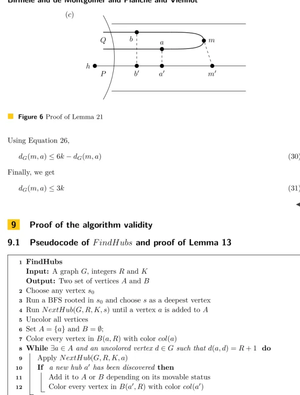
Pseudocode of F indHubs and proof of Lemma 13

1 FindHubs

Input: A graph G, integers R and K Output: Two set of vertices A and B

2 Choose any vertex s₀

3 Run a BFS rooted in s0 and choose s as a deepest vertex

4 Run N extHub(G, R, K, s) until a vertex a is added to A 5 Uncolor all vertices

6 Set A = {a} and B = ∅;

7 Color every vertex in B(a, R) with color col(a)

8 While ∃a ∈ A and an uncolored vertex d ∈ G such that d(a, d) = R + 1 do 9 Apply N extHub(G, R, K, a)

10 If a new hub a0 has been discovered then

11 Add it to A or B depending on its movable status 12 Color every vertex in B(a0, R) with color col(a0)

ILemma 22 (Computed hubs of degree 6= 2 are close to those of H). Consider a graph G

having a (r, k, `, λ) hub-laminar decomposition (H, P) with ` > 2R + 8K + 2r + 18k + 4, and a hub center h0∈ H with hub degree three or more. Suppose that F indHubs is called with a

starting node s such that s is at distance at most K + r from a hub center h with hub degree at least 3, then:

(i) For every vertex a added in A at line 8, there is a hub center h ∈ H of hub degree at least 2 at distance at most K + r from a.

(ii) For every vertex a added in A at line 12, there is a hub center h ∈ H of hub degree 1 at distance at most 2(k + r) from a.

Proof. (i) This is a direct result of lemma 9. (ii) Let f be added to A at line 12.

By induction, d is in a laminar L with endpoints h and h0, such that B(h, r) is in B(a, R). Therefore Pd,f is such that f is in L or Pd,f goes through h0.

Assume h0of degree at least 2. Then there exists a second laminar L0 incident to h0, with path P0= (h0= v₀0, v0₁, ...v0_l0). Moreover,

d(d, f ) ≥ d(d, v0_l0) ≥ d(d, h0) + d(h0, v_l00) − 2r ≥ d(d, h0) + l − 2r (32) and,

d(h0, f ) ≥ d(d, f ) − d(d, h0) ≥ l − 2r (33) As any path from d to f has a vertex in B(h0, r), h0 _{is not of degree more than 3, as} otherwise Lemma 10 (K ≥ 3k) would imply that h0 should have been detected at line 8.

By induction we deduce that there is no hub of degree more than 3 in G \ B(a, R) and that any path in G \ B(a, R) starting on d goes through the same set of hubs in the same order. This set either end with an hub of degree 1 or with the hub h (the last laminar intersects B(a, R)).

In the second case, let v0, v1, ...vz be the path associated with the laminar, and vj the

vertex closest to vz and not in B(a, R).

d(d, vj) ≥ d(d, v0) + d(v0, vj) − 2r (34) d(d, f ) ≤ d(d, vf) + k ≤ d(d, v0) + d(v0, vf) + k (35) d(d, v0) + d(v0, vf) + k ≥ d(d, v0) + d(v0, vj) − 2r (36) d(v0, vf) ≥ d(v0, vj) − 2r − k (37) d(vf, a) ≤ R + 2r + k (38) d(f, a) ≤ R + 2r + 2k (39)

In the first case, let h00 be the ending hub of degree 1 and v00₀, v₁00, ...h00 be the path associated with the laminar, by lemma 11, we have :

d(f, h00) ≤ 2k + 2r (40)

J

The following lemma is needed to prove the converse result and implies that F indHubs terminates.

ILemma 23 (Uncolored vertices are close to A). Consider a graph G having a (r, k, `, λ)

hub-laminar decomposition (H, P) with ` > 2R + 8K + 2r + 18k + 4 such that at least one hub has degree three or more.

The algorithm F indHubs ends with every vertex colored or at distance 3R + 4K at most from a vertex a of A

Proof. Let y be an uncolored vertex at distance at least 3R + 4K + 1 of a and x0 the closest colored vertex. We denote by Q = (x0, x1, ..., xt= y) the shortest path from x0 to y. All vertices in Q but x0 are then uncolored.

x0 cannot have been colored by a vertex of A, as x1would have been selected at line 8 and thus colored. x0 has therefore color lam. It cannot have been colored at Line 6 as y would then also be colored. It has therefore been colored by a path Pd,f.

x0 is at distance K of some vertex u in Pd,f, otherwise x1 would have been colored by

u. It implies that u is at distance less than 3K of d or f , otherwise x1 would have been colored at line 8. We may suppose w.l.o.g that it is at distance at most 3K from d, so that

d(d, x0) ≤ 4K.

We have that d is at distance R + 1 of some a ∈ A. Vertices added to A at line 10 have no uncolored vertex at distance R + 1. Indeed, Lemmas 9 and the size of L imply that a vertex would then have been added at line 8. By Lemma 22, a is thus at distance more than

r + K of some hub center h ∈ H, so that R > 2(K + r) implies that d is at distance at least K + r from h. By definition of an hub-laminar decomposition, d is in a laminar L, which

associated path is denoted by P = (v0= h, v1...vr).

Let vid and vi1 be vertices of P at distance less than k of d and x1. As

d(d, y) ≥ d(a, y) − d(d, a) ≥ 3R + 4K + 1 − R − 1 ≥ 2R + 4K, (41)

d(d, f ) ≥ min(d(d, y), l − 2R + 2) ≥ 2R + 4K (42) Lemma 12 thus implies that every vertex at distance k of the path vid, ...vid+2R+4K−2k is K covered by Pd,f. So i1 is either lower than id or greater than id+ 2R + 4K − 2k.

But

d(vid, vi1) ≤ d(vid, d) + d(d, x1) + d(x1, vi1) ≤ 4K + 2k + 1 (43)

d(h, vi1) ≤ d(h, vid) + 4K + 2k + 1 ≤ d(h, vid) + 2R + 4K − 2k (44) Thus, i1≤ id.

As B(vid+2R, K) disconnects L and is entirely colored, Q is entirely in L. Let us denote vij a vertex of P at distance k of xjfor every 2 ≤ j ≤ t. Then for every 1 ≤ j < t, d(vij, vij+1) ≤ 2k + 1, so that all indices ij are lower than i or all are greater than i + 2R + 4K − 2k. It

follows that they are all lower than id.

But id= d(h, vi) ≤ d(h, a) + d(a, d) + d(d, vid) ≤ 2R + 2k − r so that d(h, vit) ≤ 2R + 2k − r. Finally, d(a, y) ≤ d(a, h) + d(h, vit) + d(vit, y) ≤ R − r + 2R + 2k − r + k < 3R + 4K + 1 which is a contradiction. J ILemma 24 (Hubs of H of degree 6= 2 are close to computed ones). Consider a graph G

having a (r, k, `, λ) hub-laminar decomposition (H, P) with 2R + 7K < ` − 2r − 3k − 3 such that at least one hub of degree three or more.

When F indHubs terminates:

(i) For every hub h ∈ H of degree at least 3, there exists a vertex a in A at distance at most K + r from h.

(ii) For every hub h ∈ H of degree 1, there exists a vertex a in A at distance at most

Proof. (i) Assume that h is at distance more than max(R + r + 5K + 9k + 3, 3R + 4K) of every vertex a of A. By Lemma 23, h is of color lam. Therefore there is a path Pd,f and

vertices a, a0 in A, u in Pd,f such that :

d(d, a) ≤ R + 1 (45)

d(f, a0) ≤ R + 1 (46)

d(h, a) ≥ R + r + 5K + 9k + 3 (47)

d(h, a0) ≥ R + r + 5K + 9k + 3 (48)

d(u, h) ≤ K (49)

By combining those inequalities :

d(d, u) ≥ d(h, a) − d(d, a) − d(u, h) ≥ r + 4K + 9k + 2 (50)

d(f, u) ≥ d(h, a0) − d(d, a0) − d(u, h) ≥ r + 4K + 9k + 2 (51) By Lemma 10, there is vw ∈ E(G) and x at distance more than K + 6k from d and f such that d(x, v) = K, d(P, w) = K + 1. It results that h should have been detected at line 14 and colored by a vertex of A.

Assume that h is at distance less than R + r + 5K + 9k + 3 of a vertex a of A added at line 12. By lemma 22, there exist a hub of degree 1 of center h0 such that d(a, h0) ≤ K + r. Therefore, d(h, h0) ≤ d(h, a) + d(a, h0) ≤ R + 2r + 6K + 9k + 3, which is impossible.

Let h be at distance less than R + r + 5K + 9k + 3 of a added at line 8 of N extHub. a is at distance at most K + r of a hub h0 of degree 3 or more. We then have :

d(h, h0) ≤ R + 2r + 6K + 9k + 3 < l (52) Thus h = h0, so that h is at distance at most K + r of a.

ii) Let h be an hub of degree 1. Suppose first that h is at distance less than 3R + 4K of a vertex a of A. By a proof similar to (i), a was added at line 12 of N extHub and is at distance at most K + r of h.

Assume now that h is at distance more than 3R + 4K of every vertex a of A. Then there is a path Pd,f, and u in Pd,f at distance at most K of h. We have,

d(d, u) ≥ d(a, h) − d(a, d) − d(u, h) > 3k (53)

d(f, u) > 3k (54)

Let y and y0 be the vertices of Pd,f at distance 3k + 1 of u. Let L be the laminar having

h as an endpoint and P the path associated to L.

As 3k + 1 < l, y and y0 are in L. Let v (resp. v0) a vertex of PL at distance at most k of

y (resp. y0_{). Assume w.l.o.g that v is closest to h than v}0_.

Then v ∈ Ph,v0, which leads to a contradiction by lemma 21. Thus, h cannot be at distance more than 3R + 4K of every vertex a of A.

J ILemma (Lemma 13). Suppose that (H, P) has at least a hub of degree 3, and `(H, P) > 2R + 7K + 2r + 3k + 3. Then, for every vertex in a ∈ A, there exist a vertex in h ∈ H such

that their distance is at most K + 2r. Conversely, for every h ∈ H of degree different from 2, such a vertex a is selected in A.

9.2

Pseudocode of F indLaminars and proof of Lemma 14

1 FindLaminars

Input: A graph G, integers R and K

Output: a hub-laminar decomposition (A, Q)

2 (A, B) = F indHubs(G, R, K) 3 Q = ∅

4 Mark all vertices as deletable 5 For each vertex a of A do

6 Mark the vertices in B(a, R) as undeletable 7 For each b ∈ B do

8 Run a BFS starting at b and stopping on the first vertex a ∈ A 9 Let Q₁ be the path from b to a computed by this BFS

10 Run a BFS starting at b, not using vertices of B(Q1, K) \ (B(b, R) ∪ B(a, R)) and stopping in a

11 Let Q2 be the path from b to a computed by this BFS

12 Compute G0, the union of the connected component of G \ B(a, R) containing b

and B(a, R)

13 Color in G0 the vertices of B(a, R), B(b, R), B(Q1, K) and B(Q2, K)

14 If ∃ an uncolored vertex a in H then

15 Add a to A Mark the vertices in B(a, R) as undeletable

16 else

17 Add b to A

18 Mark the vertices in B(b, R) as undeletable

19 Delete from G the deletable vertices from B(Q₁, K) ∪ B(Q₂, K) 20 Add Q1and Q2 to Q

21 While there exists a ∈ A such that B(a, R + 1) 6= B(a, R) do

22 Run a BFS starting at a and stopping on the first vertex a0∈ A, a06= a 23 Let Q be the path from a to a0 computed by this BFS

24 If ∃w, h s.t. h ∈ r3K(Q, d(w, h) = K +1 and d(w, Q) = K +1 then 25 Add to A the first vertex h of Q satisfying the above

26 Mark the vertices in B(h, R) as undeletable

27 else

28 Add to Q the path Q from a to a0 computed by this BFS 29 Delete from G the deletable vertices from B(P, K)

ILemma (Lemma 14). Suppose that (H, P) has at least a hub of degree 3, and `(H, P) > 2R + 7K + 2r + 3k + 3. Suppose that F indLaminars is run on sets A and B returned by

F indHubs. Then it ends with every vertex deleted or marked as undeletable.

Proof. Consider the underlying decomposition (H, P) of G. Let X = {x1, . . . , xλ} be the

set of midpoints of the laminar paths (for paths of odd length, an arbitrary choice is made betwwen the two possible vertices). In the following of the proof, a laminar will be denoted by L(x), where x is the unique element of X belonging to the laminar.

A h ∈ H is said to be covered by A if there exist a vertex of A at distance at most K + 2r of h.