Visual Servoing using the Sum of Conditional Variance

(1)

HAL Id: hal-00750602

https://hal.inria.fr/hal-00750602

Submitted on 11 Nov 2012

HAL is a multi-disciplinary open access

archive for the deposit and dissemination of

sci-entific research documents, whether they are

pub-lished or not. The documents may come from

teaching and research institutions in France or

abroad, or from public or private research centers.

L’archive ouverte pluridisciplinaire HAL, est

destinée au dépôt et à la diffusion de documents

scientifiques de niveau recherche, publiés ou non,

émanant des établissements d’enseignement et de

recherche français ou étrangers, des laboratoires

publics ou privés.

Visual Servoing using the Sum of Conditional Variance

Bertrand Delabarre, Eric Marchand

To cite this version:

Bertrand Delabarre, Eric Marchand.

Visual Servoing using the Sum of Conditional Variance.

IEEE/RSJ Int. Conf. on Intelligent Robots and Systems, IROS’12, 2012, Vilamoura, Portugal.

pp.1689-1694. �hal-00750602�

(2)

Visual Servoing using the Sum of Conditional Variance

Bertrand Delabarre and Eric Marchand

Abstract— In this paper we propose a new way to achieve direct visual servoing. The novelty is the use of the sum of conditional variance to realize the optimization process of a positioning task. This measure, which has previously been used successfully in the case of visual tracking, has been shown to be invariant to non-linear illumination variations and inexpensive to compute. Compared to other direct approaches of visual servoing, it is a good compromise between techniques using the illumination of pixels which are computationally inexpensive but non robust to illumination variations and other approaches using the mutual information which are more complicated to compute but offer more robustness towards the variations of the scene. This method results in a direct visual servoing task easy and fast to compute and robust towards non-linear illumination variations. This paper describes a visual servoing task based on the sum of conditional variance performed using a Levenberg-Marquardt optimization process. The results are then demon-strated through experimental validations and compared to both photometric-based and entropy-based techniques.

I. INTRODUCTION

Visual servoing uses the information provided by a vision sensor to control the movements of a dynamic system [10], [1], [2]. This approach requires to extract and track visual information (usually geometric features) from the image in order to design the control law. This difficult tracking process is one of the bottlenecks in the development of visual servoing techniques.

Recent works have tried to circumvent these problems by using directly the information provided by the entire im-age [13], [7], [12], [4], [6]. Features are no longer extracted from the image. Those works have began with [13] and [7], where the images were reduced to eigenspaces. Later works have used directly the whole images. In [4], a control law was proposed that minimizes the error between the current image and the desired one. In that case the vector of visual feature in nothing but the image itself and the error to be regulated is the sum of squared differences (the SSD). This approach features many advantages: it does not require any matching or tracking process. Furthermore since the image measurements are nothing but the pixel intensity, there are no error in the feature extraction process leading to a very precise realization of the task.

Nevertheless, considering image intensities is quite sensi-tive to modification of the environment [4] and more robust registration function have to be considered. [3] use a full reflection model to tackle complex illumination changes thus creating the possibility to take into account some non-global illumination changes (occurrence of specularities, lighting

B. Delabarre an E. Marchand are with Universit´e de Rennes 1, IRISA, INRIA, Lagadic team, Rennes, France

{bertrand.delabarre,marchand}@irisa.fr

direction non constant wrt. the surface, etc). But this method is limited since the range of application only applies to illumination conditions that can be represented with the con-sidered model. A more recent approach also concon-sidered the mutual information [15] as the similarity measure between desired and current images [6]. This information theoretic method allows to servo the camera in order to maximize the quantity of information shared by the current and desired image (that is the mutual information which is build by a measure of image entropy [15]). The approach is therefore well suited for a large range of variations such as occlusions, specularities and even different modality images. A drawback of this method is that it is quite complex to compute and therefore computationally expensive.

In this paper we propose a compromise between this two branches. Our method is based on the sum of condi-tional variance, a measure using the probability distribution functions of the luminance in the image to adapt a tem-plate. When considering direct visual servoing method, the choice of the similarity function is fundamental. Between the simplest alignment function that is the sum of squared differences [4] and the mutual information [6], one can consider other metric such as the Zero-mean Normalized Cross Correlation (or ZNCC [11]) which has proved to be very robust to linear brightness variation [8] thanks to the normalization embodied into the ZNCC. In this paper, to be able to handle non-linear brightness variation and to have a low computational complexity, we propose to consider, as a similarity function, the sum of conditional variance (or SCV). With respect to the simple SSD function, SCV allows to dynamically adapt the reference image to the illumination conditions of the current image acquired by the camera. The reference image is replaced by an expected image computed using a probabilistic expectation operator (that take into account illumination condition in both current and learned desired image). Let us note that this approach has proved recently to be very efficient in a tracking context as demonstrated in [14].

Dynamically adapting the desired image makes the ap-proach able to tackle brutal illumination variations. Further-more, this approach is computationally very efficient since it is still based on a simple difference between pixels. It is also easy and fast to compute which makes it a good solution for visual servoing tasks involving illumination variations of the scene.

In this paper we will first have a quick reminder of the direct visual servoing methods before describing the new method based on the sum of conditional variance. Several experiments are then exposed, showing the advantages and

(3)

limitations of the approach.

II. DIRECTVISUALSERVOING

A. Positioning Task

The aim of a positioning task is to reach a desired pose of the camera r∗, starting from an arbitrary initial pose. To achieve that goal, one needs to define a cost function that reflects, in the image space, this error. Most of the time this cost function f is an error measure which needs to be minimized. Considering the actual pose of the camera r the problem can therefore be written as an optimization process:

br = arg min_r f (r, r

∗₎ ₍₁₎

where _br, the pose reached after the optimization process (servoing process), is the closest possible to r∗ (optimally br = r

∗_{). For example, considering a set of geometrical}

features s, the task will typically have to minimize the difference between s(r) and the desired configuration s* which leads to:

b

r = arg min

r (s(r)− s

∗_). ₍₂₎

This visual servoing task is achieved by iteratively applying a velocity to the camera. This requires the knowledge of the interaction matrix Ls of s(r) that links the variation of ˙s to

the camera velocity and which is defined as:

˙s(r) = Lsv (3)

where v is the camera velocity.

This equation leads to the expression of the velocity that needs to be applied to the robot. The control law is classically given by:

v =_−λL+_s(s(r)_{− s}∗) (4) where λ is a positive scalar.

B. Photometric visual servoing

In the case of direct visual servoing, the feature s becomes the image itself (s(r) = I(r)). This means that the optimiza-tion process becomes [4]:

br = arg min_r (I(r)− I

∗₎ ₍₅₎

where I(r) and I∗ are respectively the image seen at the position r and the template image (both of N pixels). The control law is inspired by the Levenberg-Marquardt (LM) optimization approach. It is given by:

v =_−λ(HI+ µ diag(HI))−1LI(I(r)− I∗) (6)

where λ and µ are positive scalars where HI= LITLI and

LI is the interaction matrix which can be expressed as:

LI=−∇ITLx (7)

and Lxis the interaction matrix of a point (see details in [4]).

III. VISUAL SERVOING USING THESUM OF

CONDITIONALVARIANCE

A. Sum of Conditional Variance

The works of [4] used the sum of squared differences to perform direct visual servoing. The main drawback of this method is that it is based on the hypothesis that the luminance of a point does not vary with time:

I(x + dx, t + dt) = I(x, t) (8) where x represents the pixel coordinates and dx the motion underwent by the image during the laps of time dt. When performing a visual servoing task, this hypothesis is often violated and, as the light changes in the scene, the task can quickly fail. This is the reason why this paper describes a visual servoing process using the Sum of Conditional Variance (SCV), a measure which was used in [14] to track planar object using a KLT like approach with very good results in illumination-varying conditions. As in our case, this measure was used in [14] because it no longer relies a simple difference between current and a reference image (or template image). Indeed, the template is dynamically adapted to the illumination conditions of the current image seen at each new iteration. To adapt the template, an expected image ˆ_{I is defined as:}

ˆ_{I(x) =}_{E(I(x) | I}∗_(x)) ₍₉₎

where_{E is an expectation operator and x a pixel in the image.} With this expected template computed, a good correlation measure is given by:

SCV =X

x

(I(x)_{− ˆI(x)).} (10)

The expected image ˆI is computed from the joint proba-bility distribution between I and I∗. Those probabilities are computed from the empirical analysis of I and I∗. As they both have the same dynamic d, which usually is 256, for each couple of grey levels i in I and j in I∗ it is possible to compute: PII∗(i, j) = P (I(x) = i , I∗(x) = j ) (11) = 1 N X x φ(I(x)_{− i)φ(I}∗(x)_{− j ) (12)} where φ(a) equals 1 if a=0, 0 otherwise and PII∗represents

the probability that a pixel x takes the value i in I and j in I∗. From this joint probability distribution, the probability distributions of I∗ can easily be found. For example the probability distribution for the apparition of a grey level j in I∗ is given by:

PI∗(j) =

X

i

PII∗(i, j). (13)

From this probability distribution functions the computation of the expected grey levels in ˆI becomes, for each grey level j in I∗_: ˆ_{I(j ) =}X i iPII∗(i , j ) PI∗(j ) . (14)

(4)

Template

Patch

Sum of Squared Differences Mutual information Sum of Conditional Variance

-10 -5 0 5 10-10 -5 0 5 10 0 5e+06 1e+07 1.5e+07 2e+07 2.5e+07 3e+07 tx ty 0 5e+06 1e+07 1.5e+07 2e+07 2.5e+07 3e+07 -10 -5 0 5 10-10 -5 0 5 10 0.1 0.2 0.3 0.4 0.5 0.6 0.7 0.8 tx ty 0.1 0.2 0.3 0.4 0.5 0.6 0.7 0.8 -10 -5 0 5 10-10 -5 0 5 10 0 5e+06 1e+07 1.5e+07 2e+07 2.5e+07 tx ty 0 5e+06 1e+07 1.5e+07 2e+07 2.5e+07

Fig. 1. Cost function in nominal case. Here the displayed current patch is the one resulting of tx = 0 and ty = 0 pixel.

Template

Patch

Sum of Squared Differences Mutual information Sum of Conditional Variance

-10 -5 0 5 10-10 -5 0 5 10 4.9e+07 5e+07 5.1e+07 5.2e+07 5.3e+07 5.4e+07 5.5e+07 5.6e+07 5.7e+07 5.8e+07 5.9e+07 tx ty 4.9e+07 5e+07 5.1e+07 5.2e+07 5.3e+07 5.4e+07 5.5e+07 5.6e+07 5.7e+07 5.8e+07 5.9e+07 -10 -5 0 5 10-10 -5 0 5 10 0.04 0.06 0.08 0.1 0.12 0.14 0.16 0.18 0.2 0.22 0.24 tx ty 0.04 0.06 0.08 0.1 0.12 0.14 0.16 0.18 0.2 0.22 0.24 -10 -5 0 5 10-10 -5 0 5 10 0 200000 400000 600000 800000 1e+06 1.2e+06 1.4e+06 1.6e+06 tx ty 0 200000 400000 600000 800000 1e+06 1.2e+06 1.4e+06 1.6e+06

Fig. 2. Cost function when the light has been significantly lowered. The displayed current patch is the one resulting of tx = 0 and ty = 0 pixel.

B. Analysis of the SCV cost function

In order to assess the suitability of the sum of conditional variance in the case of illumination changes, a comparison of various similarity functions was realized. The comparison between two images (a reference image and a current image) follows the following pattern. On the images, a patch of 100x100 pixels is selected. The patch is extracted from the reference image, creating a reference template. In the current image, patches are extracted by moving a 100x100 window, starting from a translation (tx,ty) equal to (-10,-10) pixels with relation to the position of the template and finishing with (tx,ty) equal to (10,10) pixels. The cost function is then computed between each patch extracted and the template, leading to the shape of the cost function.

When computing the cost functions, histogram binning was used (see more details in section IV-A). The mutual information was computed with 8 bins as in [6] and the sum of conditional variance with 64 bins. A first comparison was made with both the current and reference image being the same, creating a baseline (see fig 1). This shows the shapes of the functions in the ideal case were the conditions do not vary during the visual servoing. The three cost functions possess a marked optimum when (tx,ty) equals to (0,0) pixels. They also present a smooth shape and no local extrema which make them well suited for optimization processes in nominal conditions. With that baseline established, a second comparison was made. For this comparison, the current image was not the same as the reference but had undergone a variation of the luminance rendering it darker than the reference (see fig 2). This time, the shape of the SSD is greatly impacted with a flatten area resulting in a significant shift in the extremum location which means it is not suitable for an optimization process in this conditions. The MI and SCV on the other hand show only a small attenuation of

the slopes around their optimum but stay sharp enough to assure convergence toward the correct position during an optimization process.

Obviously, this analysis considers only 2 dof, whereas in the visual servoing experiments considered in this paper, the 6 camera dof are controlled. Nevertheless these experiments (along with other which can be found in [14]) allow to illus-trates that SCV is far less sensitive than SSD to illumination variations.

C. SCV-based control law

Using the SCV to measure the difference between I(r) and ˆI the optimization process becomes:

br = arg min_r (I(r)− ˆI). (15) Considering the LM approach shown in equation (6), the control law becomes:

v =_−λ(HS+ µ diag(HS))−1LSCV(I(r)− ˆI) (16)

where HS = LSCVTLSCV and LSCV is the interaction

matrix associated to the task. Only illumination variations (and not camera pose) impact ˆI the interaction matrix matrix can be chosen as in [4]: LSCV= ∂I(r) ∂r =−∇I(r) T_L x. (17)

IV. EXPERIMENTALVALIDATIONS

A. Histogram Binning

To compute the probability distribution functions used by the SCV and compute for each new frame the new reference image ˆI, histogram binning was used. This was done both to smooth the resulting image ˆI and to decrease the computation time in order to enhance the quality of the servoing task. To

(5)

I

I∗

8 bins 64 bins 256 bins

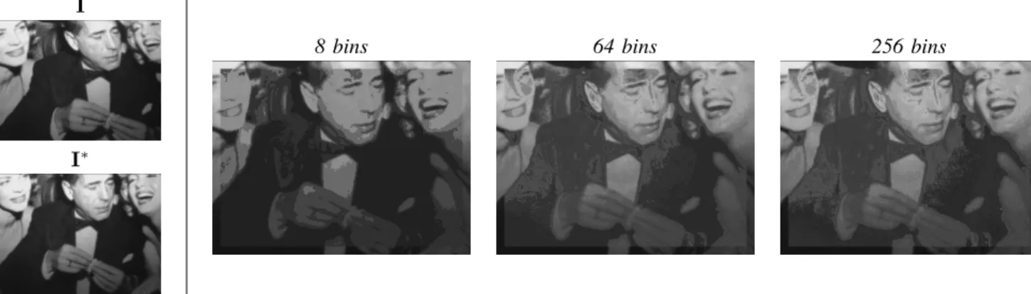
Fig. 3. Influence of the number of bins on the predicted image when far from reach. On the left, with 8 bins the image is flattened and has lost a lot of high frequencies. 256 bins introduces more noise when the difference between I and I∗increases than 64. The frame on the borders represent the area in the image which is not included in the computation.

compute such histograms a number of bins N c is set, then the source image is scaled:

I(x) = I(x)(N c− 1)

d_{− 1} . (18)

The histograms are then computed on this scaled image which dynamic is N c, ensuring that they are composed of only N c bins. An other reason for choosing not to use the full dynamic of the image is that computing probabilities from the histograms as in (14) results in approximating them. This is the case because an empirical observation of a probability distribution function does not necessarily equal its ’real’ distribution. The main problem with those approached probabilities is that they can result in noise in the predicted image when using an important number of bins. On the other hand, if the chosen number of bins is too low, the resulting image loses a lot of details. See figure (3) for examples.

It is also interesting to note that as the number of bins decreases, so does the precision of the positioning task since more high frequency details are lost. This is why during, the servoing task the number of bins is adapted dynamically. First, the binning is done using 64 bins as the level of detail in the image is sufficient with this number of bins and increases to 256 when close from reach to get more precision. To do that, the value of the SCV at the beginning of the task is kept in memory and the switch is effected when the current SCV reaches a certain percentage of that value. B. First Experiment: Nominal case

The first experience aims to analyze the behaviour of the SCV approach in a classical case. The positioning task controls all 6 degrees of freedom. The interaction matrix during the servoing is computed assuming that the Z coordinate of each point is constant, in this case it assumed as equal to 70 cm. As for the λ and µ parameters of the optimization, they were empirically chosen as 4 and 0.001 respectively. For the initial pose, the difference was ∆r = {16cm, −20cm, 6cm, −0.27rad, −0.19rad, −0.09rad} with relation to the desired pose. Figure 4 shows the behaviour of the model during the optimization process. In

the error image between the current and expected images, a pixel of luminance l=128 (grey pixel) means there is no difference between the two images. The graphics show the evolution of a chosen parameter with relation to the iterations of the algorithm.

Several observations can be made concerning this first experiment. First, the task converges, leading the robot to the good position with a good precision of ∆r∗= {0.07mm, 0.16mm, 0.01mm, 1e−4_{rad, 2e}−5_{rad, 1e}−4_rad_}.

The second observation is that the evolution of the camera location is smooth. The SCV also vanishes without being noisy, showing that the SCV is well suited in this case.

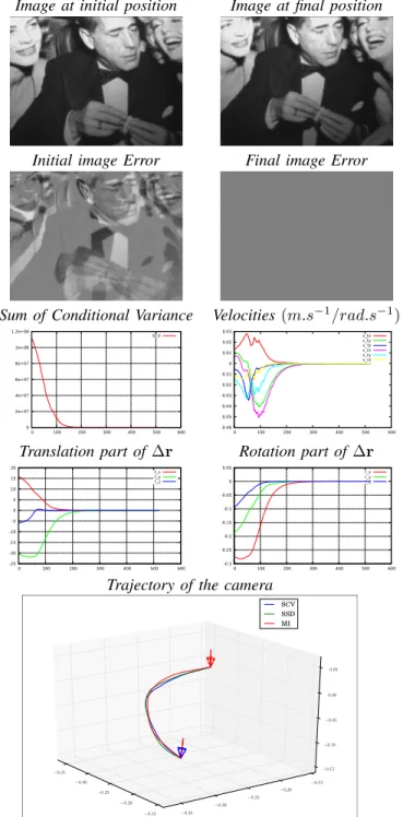
C. Second Experiment: Robustness with relation to illumi-nation changes

The goal of this experiment is to show the robustness of our method towards illumination variations in the scene. In order to do that, after acquiring the image at the desired position, the servoing is launched after the lights have been attenuated. The results of this experiment are exposed on figure 5. The initial position was a little bit less complicated with a difference of ∆r = {14cm, −18cm, 1cm, −0.28rad, −0.18rad, −0.03rad} from the desired position, which is still a consequent movement.

In these conditions, the servoing task still converged, thanks to the adaptation of the predicted image to the current one as we can see on figure 5. The final position was reached with a precision of ∆r∗ = {0.4mm, 0.8mm, 0.9mm, 1e−3_{rad, 4e}−4_{rad, 1e}−3_rad

} which gives a distance to the desired position of 1.3mm. It is slightly less precise than in the nominal case but it was still a good result compared to the other methods since the SSD diverged and the mutual information showed a repositioning precision of 2.4mm. The graph of SCV also shows around iteration 300 the change in the number of bins which caused an improvement in the precision without impacting the convergence of the task.

(6)

Image at initial position Image at final position

Initial image Error Final image Error

Sum of Conditional Variance Velocities (m.s−1/rad.s−1)

0 2e+07 4e+07 6e+07 8e+07 1e+08 1.2e+08 0 100 200 300 400 500 600 SCV -0.06 -0.05 -0.04 -0.03 -0.02 -0.01 0 0.01 0.02 0.03 0 100 200 300 400 500 600 v_tx v_ty v_tz v_rx v_ry v_rz

Translation part of∆r Rotation part of ∆r

-25 -20 -15 -10 -5 0 5 10 15 20 0 100 200 300 400 500 600 t_x t_y t_z -0.3 -0.25 -0.2 -0.15 -0.1 -0.05 0 0.05 0 100 200 300 400 500 600 r_x r_y r_z

Trajectory of the camera

−0.35 −0.30 −0.25 −0.20 −0.15 −0.35 −0.30 −0.25 −0.20 −0.15 −0.15 −0.10 −0.05 0.00 0.05 SCV SSD MI

Fig. 4. Behaviour of the model in a classical case.

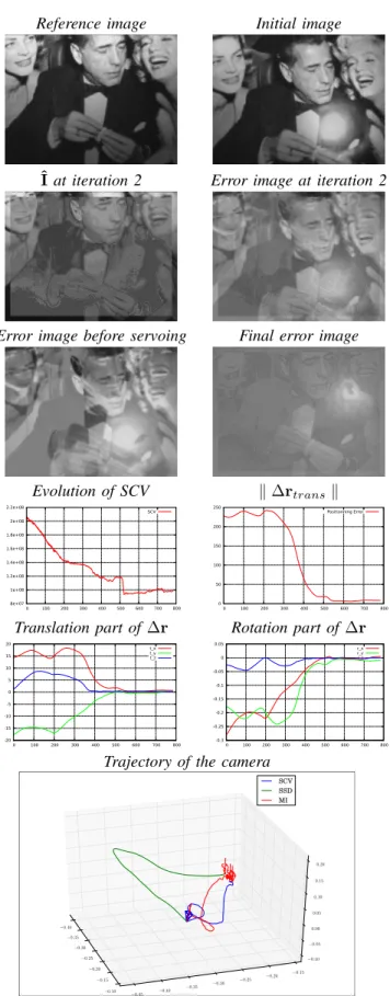
D. Third Experiment: Case of a specularity

Finally, a last experiment was done to show the behaviour of the SCV when confronted to specularities. The SCV is not really suited for this purpose, as local variations will change the global probabilities therefore areas where no variations occurred will be treated as areas where variations occurred which will create incoherences in the predicted image. But even if the measure is impacted by specularities, it is interesting to see how the servoing task reacts when confronted to the situation. To realize the experiment, the task was launched again from the position described in

Reference image Initial image

ˆ_{I at iteration 2} _{Error image at iteration 2}

Error image before servoing Final error image

Evolution of SCV _{k ∆r}transk 0 200000 400000 600000 800000 1e+06 1.2e+06 1.4e+06 1.6e+06 1.8e+06 2e+06 2.2e+06 0 100 200 300 400 500 600 700 SCV 0 50 100 150 200 250 300 350 0 100 200 300 400 500 600 700 Positionning Error

-30 -25 -20 -15 -10 -5 0 5 10 15 20 0 100 200 300 400 500 600 700 t_x t_y t_z -0.4 -0.35 -0.3 -0.25 -0.2 -0.15 -0.1 -0.05 0 0.05 0 100 200 300 400 500 600 700 r_x r_y r_z

−0.45 −0.40 −0.35 −0.30 −0.25 −0.20 −0.15 −0.10 −0.40 −0.35 −0.30 −0.25 −0.20 −0.15 −0.10 −0.05 −0.05 0.00 0.05 0.10 0.15 0.20 0.25 0.30 SCV SSD MI

Fig. 5. Behaviour of the model in a the case of illumination variations. The evolution of the SCV shows around iteration 210 gain in precision thanks to the increase in the number of bins used.

section IV-C. Then the servoing task was launched while a light was pointed directly at the non-lambertian surface,

(7)

Reference image Initial image

ˆ_{I at iteration 2} _{Error image at iteration 2}

Error image before servoing Final error image

Evolution of SCV _{k ∆r}transk 8e+07 1e+08 1.2e+08 1.4e+08 1.6e+08 1.8e+08 2e+08 2.2e+08 0 100 200 300 400 500 600 700 800 SCV 0 50 100 150 200 250 0 100 200 300 400 500 600 700 800 Positionning Error

-20 -15 -10 -5 0 5 10 15 20 0 100 200 300 400 500 600 700 800 t_x t_y t_z -0.3 -0.25 -0.2 -0.15 -0.1 -0.05 0 0.05 0 100 200 300 400 500 600 700 800 r_x r_y r_z

−0.40 −0.35 −0.30 −0.25 −0.20 −0.15 −0.10 _−0.45 −0.40 −0.35 −0.30 −0.25 −0.20 −0.15 −0.10 −0.05 0.00 0.05 0.10 0.15 0.20 SCV SSD MI

Fig. 6. Behaviour of the model in a the case of a specularity in the image.

creating a specularity in the image. The results of this experiment are shown on figure 6.

The predicted image is directly impacted, as the variations

in the probability distribution functions due to the specularity are applied to the whole considered area. The evolution of the SCV is also impacted, as the specularity in the image moves depending on the position of the camera. But even though it is lessprecise than in the nominal case, the task still converges with a distance to the goal position of 9mm when the SSD ends up at 15mm in the same conditions and the mutual information at 4mm. The analysis of_{k ∆r}transk

is really interesting as it shows a shift in the minimum of the SCV because the robot came closer to the desired position before converging with a greater repositioning error.

V. CONCLUSION

In this paper we described a new way to achieve direct visual servoing. This approach is based on a similarity measure issued from the information theory called the sum of conditional variance (SCV). Compared to photometric visual servoing method [4], it performs similarly in nominal cases, when large occlusions or specularities appear in the scene and better when the illumination conditions are non-locally changing. Compared to mutual information based visual servoing [6], the range of application is narrower for the SCV as it is less robust towards local variations and is not multi-modal. But it is easier to compute and less computationally expensive when the number of bins used for the servoing task increases. This makes it a very good compromise when performing direct visual servoing. As SCV is computed based on the image histograms, it is non-invariant to local changes. This problems could be addressed for example by using sub-regions histograms as it was mentioned in [9] or using M-estimators in the control law [5].

REFERENCES

[1] F. Chaumette, S. Hutchinson. Visual servo control, Part I: Basic approaches. IEEE Robotics and Autom. Mag., 13(4):82–90, Dec. 2006. [2] G. Chesi, K Hashimoto, editors. Visual servoing via advanced

numerical methods. LNCIS 401. Springer, 2010.

[3] C. Collewet and E. Marchand. Modeling complex luminance variations for target tracking. In IEEE CVPR’08, Anchorage, June 2008. [4] C. Collewet and E. Marchand. Photometric visual servoing. IEEE

Trans. on Robotics, 27(4):828–834, August 2011.

[5] A.I. Comport, E. Marchand, F. Chaumette. Statistically robust 2D visual servoing. IEEE T. on Robotics, 22(2):415-421, aprilAvril 2006.. [6] A. Dame and E. Marchand. Mutual information-based visual servoing.

IEEE Trans. on Robotics, 27(5):958–969, October 2011.

[7] K. Deguchi. A direct interpretation of dynamic images with camera and object motions for vision guided robot control. IJCV, 37(1), 2000. [8] L. Di Stephano, et al. ZNCC-based template matching using bounded

partial correlation. Pat. Rec. Letters, 26:2129–2134, 2005.

[9] G. Hermosillo, C. Chefd’hotel, O. Faugeras. Variational methods for multimodal image matching. IJCV, 50:329–343, Dec. 2002. [10] S. Hutchinson, G. Hager, P. Corke. A tutorial on visual servo control.

IEEE T. on Robotics and Automation, 12(5):651–670, October 1996. [11] M. Irani and P. Anandan. Robust multi-sensor image alignment. In

IEEE ICCV’98, pages 959–966, Bombay, India, 1998.

[12] V. Kallem, et al. Kernel-based visual servoing. IEEE/RSJ IROS’07, pp. 1975–1980, San Diego, 2007.

[13] S.K. Nayar, S.A. Nene, and H. Murase. Subspace methods for robot vision. IEEE T. on Robotics, 12(5):750 – 758, Oct. 1996.

[14] R. Richa, R. Sznitman, R. Taylor, and G. Hager. Visual tracking using the sum of conditional variance. In IEEE IROS’11, pages 2953–2958, San Francisco, Sep. 2011.

[15] C.E. Shannon. A mathematical theory of communication. SIGMOBILE Mob. Comput. Commun. Rev., 5(1):3–55, January 2001.