A computer model for the heat losses in the exhaust manifold of an internal combustion engine

IN THE EXHAUST MANIFOLD OF AN INTERNAL COMBUSTION ENGINE

by

Richard Milton Frank B.Sc. Mechanical Engineering

Cornell University (1974)

SUBMITTED IN PARTIAL FULFILLMENT OF THE REQUIREMENTS OF THE

DEGREE OF MASTER OF SCIENCE

IN

MECHANICAL ENGINEERING at the

MASSACHUSETTS INSTITUTE OF TECHNOLOGY May 1986

Copyright Massachusetts Institute of Technology, 1986

Volume I Signature of Author: Certified by: Accepted by: Chairman

Archives

Signature redacted

Department of Mechanical Engineering May 1986

Signature redacted

.Jack A. Ekchian

- hesis Supervisor

Signature redacted

Prof. Ain A. Sonin Departmental Committee on Graduate Students Department of Mechanical Engineering

14ASSCHUSESTiTUTE

JUL 28 1986

A COMPUTER MODEL FOR THE HEAT LOSSES IN THE EXHAUST MANIFOLD OF AN

INTERNAL COMBUSTION ENGINE

by

Richard M. Frank

Submitted to the Department of Mechanical Engineering on May 9, 1986 in partial fulfillment of the requirements for the Degree of Master of Science

in Mechanical Engineering

ABSTRACT

A model was developed for the exhaust manifold of an internal

combustion engine for use in a computer simulation program. Previous experimental work that developed heat transfer correlations for the port is combined with other general empirical correlations for turbulent pipe flow to give an overall heat transfer model for the manifold. The model developed has the advantages of being applicable to engines of varying numbers of cylinders and displacement while remaining simple.

Correlations are also included to accept different geometries and materials for the manifold piping. The model has been applied to a turbocompounded diesel simulation program being developed at the Massachusetts Institute of Technology. The model was validated by comparing predicted performance to test results from a specially instrumented turbocharged engine with thermocouples located along one section of the exhaust manifold. The results of a study done into the effects of exhaust manifold insulation on engine performance are

presented. Examples of the output for this program, including both heat transfer and pressure drop data for various exhaust manifold designs, are included with this thesis.

Thesis Supervisor: Dr. Jack A. Ekchian

ACKNOWLEDGEMENTS

It's a special pleasure to acknowledge the direct contributions to this work of three people. The first is that of my advisor Jack

Ekchian. His patience and guidance were greatly appreciated. The second is that of Professor John Heywood who always seemed to find the time to help when things weren't going right. Finally, is the great help provided to me by my partner Dennis Assanis. He answered alot of questions.

There are too many people to list whose indirect contributions also had a significant impact on getting this work completed. Suffice it to say that the unflagging support of my family and my friends both inside and outside of the Sloan Automotive Lab has been greatly appreciated.

A special thanks goes to Kevin Hoag, Chris Moore, and Cummins Engine Company for their colaboration in providing the experimental results. Without them Chapter 7 never would have existed.

The computer code printed in Volume II is the result of the efforts of many people. They have been recognized in the subroutines where

their work is represented.

This thesis is dedicated to my Grandparents, Mr. and Mrs. Leon Frank Sr. and Mr. and Mrs. Harold Wallace. I'll always wish that I could have known them better.

This work has been supported by the DOE Heavy Duty Transport

Technology Program under NASA Grant 3-394, the M.I.T. Consortium on the Use of Ceramic Materials in Internal Combustion Engines, and by TRW. Their contributions and support are gratefully appreciated.

TABLE OF CONTENTS VOLUME 1 ABSTRACT ... ACKNOWLEDGEMENTS ... LIST OF TABLES ... LIST OF FIGURES ... CHAPTER 1. INTRODUCTION ... 2. GEOMETRICAL MODEL ...

3. MANIFOLD HEAT TRANSFER ... 3.1 Port Heat Transfer: ... 3.2 Other Sections of the Manifold: 3.2.1 Entrance Effects ...

3.2.2 Effect of Curved Pipe 3.2.3 3.2.4 3.2.5 Effect Surface Viscous of Variable Roughness Heating Gas Properties ... 0.... .. 0... 3.2.6 Summary ...

3.3 Steady-State Heat Transfer Through a Composite Wall 3.4 Determination of the Inside Wall Temperature ...

3.4.1 Steady-State Wall Temperature Determination 3.4.2 Transient Temperature Calculations ... 3.5 Turbine Connecting Pipe Heat Transfer ...

PAGE 2

3

7

8

30

33

35

35

37

38

39

4. PRESSURE LOSSES ... 5. THERMODYNAMIC EQUATIONS ...

5.1 General Equations ... 5.2 Solution of the Equations ...

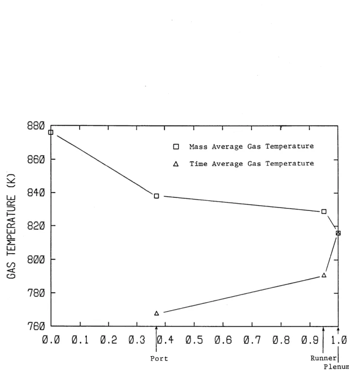
5.3 Time Average vs. Mass Average Temperatures 6. MODEL APPPLICATION AND BEHAVIOR ...

6.1 Manifold Configuration ...

6.2 Initial Calibration of the Engine ... 6.3 Boundary Conditions for the Exhaust Manifold 6.4 Behavior of a Representative Run ...

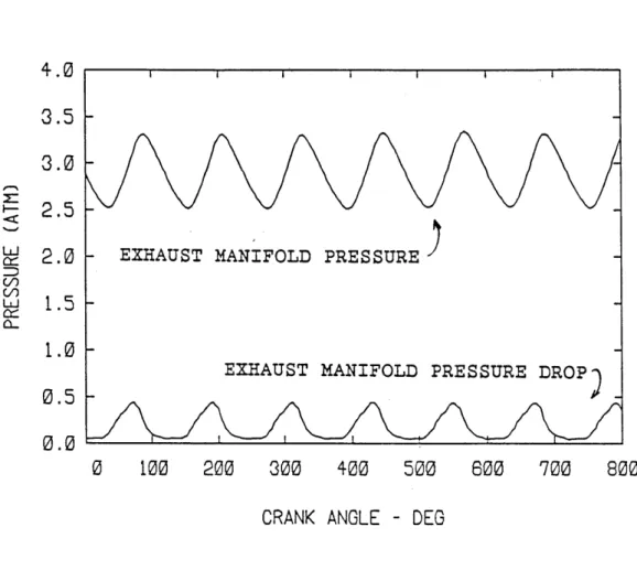
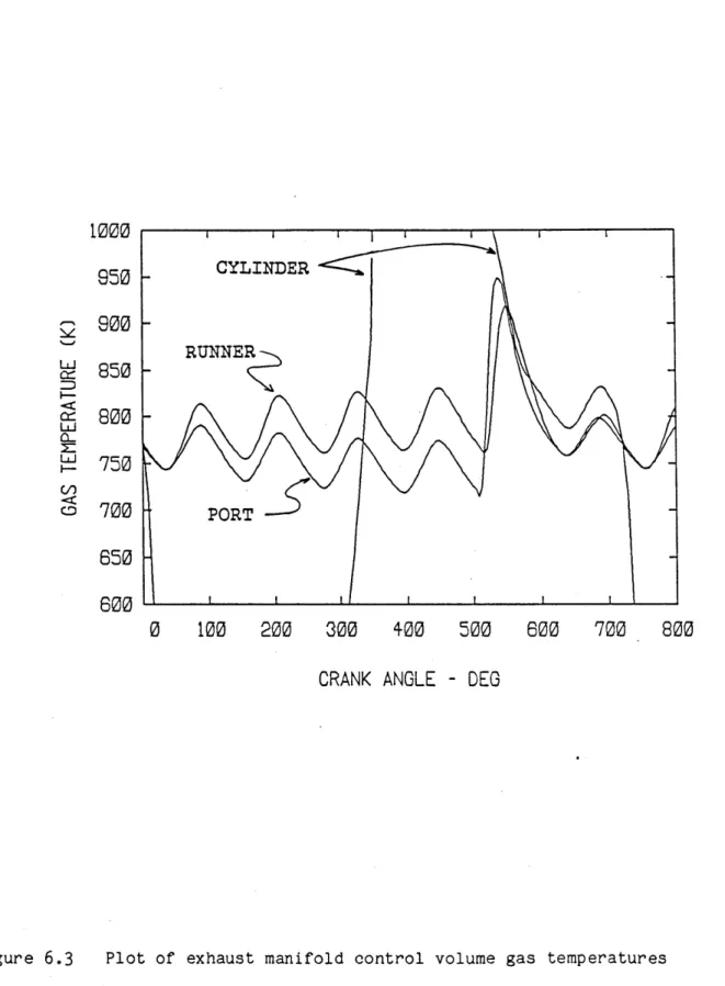
6.4.1 Manifold Pressure and Pressure Drop ... 6.4.2 Mass Flow Along Exhaust Manifold ... 6.4.3 Exhaust Manifold Gas Temperatures... 6.4.4 Plenum and Averaged Manifold Gas Temper

6.4.5 Manifold Heat Transfer Coefficients ... 6.4.6 Heat Transfer Rates ... 6.5 Problems With the Turbomachinery Maps ... 6.6 Time Averaged vs. Mass Averaged Temperatures 6.7 Distribution of heat losses in the exhaust 6.8 Distribution of energy in the engine ... 7. 8 CYLINDER TURBOCHARGED ENGINE EXPERIMENT ...

7.1 Description ... 7.2 Description of simulation model ... 7.3 Calibration of the engine simulation ... 7.4 Manifold temperature predictions vs.

7.5 Predicted thermocouple temperatures

ature. measurements

... 0...

8. PARAMETRIC STUDIES ... 76

8.1 Basic Assumptions ... 76

8.2 Effect of Decreased Manifold Heat Transfer on Gas Temperatures ... 77

8.3 Effect of Exhaust Manifold Insulation on Engine Performance ... 78

8.3.1 Normal cylinder heat transfer ... 80

8.3.2 Partially insulated cylinder ... 81

8.4 Effect of Transient Wall Temperatures on Predicted Performance ... 82 9. CONCLUSIONS ... 85 REFERENCES ... 87 TABLES ... 89 FIGURES ... 98 VOLUME 2 TABLE OF CONTENTS... 123 APPENDIX A. PROGRAMING INFORMATION... 126

B. SUMMARY OF CHANGES MADE TO PROGRAM... 131

C. LISTING OF PROGRAM... 135

D. SAMPLE INPUT FILES FOR COMPUTER CODE... 310

LIST OF TABLES Table 6.1 Table 6.2 Table 6.3 Table 6.4 Table 7.1 Table 7.2 Table 8.1 Table 8.2 Table 8.3

Engine specifications - Cummins 6 cylinder NH

engine. ...

Initial calibration of 6 cylinder engine

peak torque - two engine speeds...

Initial calibration of 6 cylinder engine

1600 RPM - 50% and 25% loads...

Time average vs. mass average exhaust gas

temperatures...

Engine specifications - Cummins 8 cylinder 903

engine...

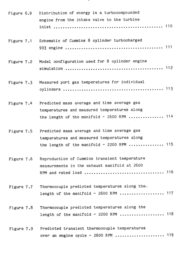
Initial calibration of 8 cylinder engine at

peak torque - 2200 and 2600 RPM...

Three levels of exhaust insulation - normal

cylinder heat transfer...

Three levels of exhaust insulation - partially

insulated cylinder...

Steady-state vs. transient wall temperature

engine performance predictions... 89 90 91 92

93

LIST OF FIGURES Figure 1.1 Figure 2.1 Figure 2.2 Figure 3.1 Figure 6.1 Figure 6.2 Figure 6.3 Figure 6.4 Figure 6.5 Figure 6.6 Figure 6.7 Figure 6.8

Schematic of turbocompounded engine ... 98

Simplest form of exhaust manifold model ... 99

Typical head arrangement with two exhaust

valves per cylinder ...

Entrance effects on heat transfer in turbulent

pipe flow ...

Plot of manifold pressure and pressure drop

over an engine cycle ...

Plot of mass flow betwen exhaust manifold

control volumes over an engine cycle ...

Plot of exhaust manifold control volume gas

temperatures over an engine cycle ...

Plot of plenum and average manifold gas

temperatures over an engine cycle ...

Plot of manifold heat transfer coefficients

over an engine cycle ...

Plot of manifold heat transfer rates over an

engine cycle ...

Mass average and time average gas temperatures

along the exhaust flow path in the manifold ...

Distribution of heat losses in the exhaust

manifold ... 100 101 102 103 104 105 106 107 108 109

Figure 6.9 Figure 7.1 Figure 7.2 Figure 7.3 Figure 7.4 Figure 7.5 Figure 7.6 Figure 7.7 Figure 7.8 Figure 7.9

Distribution of energy in a turbocompounded engine from the intake valve to the turbine

inlet ...

Schematic of Cummins 8 cylinder turbocharged

903 engine ...

Model configuration used for 8 cylinder engine

simulation ...

Measured port gas temperatures for individual

cylinders ... 110

111

112

113

Predicted mass average and time average gas temperatures and measured temperatures along

the length of the manifold - 2600 RPM ... 114

Predicted mass average and time average gas temperatures and measured temperatures along

the length of the manifold - 2200 RPM ... 115

Reproduction of Cummins transient temperature measurements in the exhaust manifold at 2600

RPM and rated load ... 116

Thermocouple predicted temperatures along

the.-length of the manifold - 2600 RPM ... 117

Thermocouple predicted temperatures along the

length of the manifold - 2200 RPM ...

Predicted transient thermocouple temperatures

over an engine cycle - 2600 RPM ... 118

Figure 8.1

Figure 8.2

Effect of exhaust manifold insulation on reciprocator exhaust gas temperature and

turbocharger turbine inlet temperature ... 120

Port gas temperature and port transient wall

CHAPTER 1. INTRODUCTION

In the past decade there has been a strong increase in interest in computer simulation of internal combustion engine operation and

performance. This interest has been due to the increased sophistication of today's engines where it is necessary to minimize pollutants and maximize economy. The rapidly increasing power of computers to carry out large calculations has aided this effort. The rational behind computer simulation programs is that if they can be written to accurately predict the performance of existing engines, then they can eventually be applied to study possible design modifications of internal combustion engines without building the engine. As a design tool, a computer simulation program can be used to predict the potential benefit, if any, that a given engine modification will have on the emissions or performance of an internal combustion engine.

One promising design modification to internal combustion engines that is currently of interest is lower heat rejection through the use of ceramic materials. Since ceramic materials can withstand much higher operating temperatures than metals, the use of ceramics in engines can be very attractive. An engine computer simulation code is a valuable tool for studying the usefulness of ceramics in internal combustion engines. The results can be used to indicate where ceramics would be most effective in improving engine performance and just as importantly to help define those areas where the use of ceramics would not provide any improvement in engine performance.

engine which predicts performance over a range of conditions. These models are linked in the simulation to calculate the expected

performance of the engine as a whole. The more accurately the components of the engine are represented, the better a simulation program is able to predict actual engine performance.

In the simulation of turbocharged engines, one important component of the engine which needs to be modelled is the exhaust manifold. The exhaust manifold of the engine is especially difficult to model because of its complex shape and flow characteristics. It is important to be able to quantify the losses in the manifold, due to heat transfer and flow friction and to determine the energy available at the inlet to the turbine for the extraction of usable work. Since low heat rejection engines are expected to be turbocharged, it is important that a simulation code for these engines include an accurate model for the exhaust manifold.

Previous models for exhaust manifolds used in computer simulation programs were often limited to either accounting for heat transfer or pressure fluctuations in the manifold but not both. Often, the manifold was modelled as a single plenum with uniform properties. With such a lumped parameter model it is not possible to account for the variation

in losses along the length of the manifold due to the change in conditions with respect to position in the manifold. In these

simulations, it was usually necessary to define the wall temperature along the manifold a priori. In order for the simulation to be useful

to predict the performance of engines yet to be built, it is necessary to predict the wall temperatures that would result for a given exhaust manifold shape and wall composition.

The immediate purpose of the present study was to develop a model for inclusion in an overall engine simulation currently being written at MIT. The primary goal of this engine simulation is to simulate the

operation of a turbocompounded diesel engine. Given the engine size, materials of construction, and the engine operating speed and load the program provides an output that predicts the performance of the entire system. In this simulation, all conditions are assumed to be steady-state.

The simulation is expected to be especially useful in predicting the performance gains or losses associated with changes in material such as the use of ceramic linings or changes in components such as different turbochargers. The simulation has been in operation since 1984 and the current thrust has been to upgrade the heat transfer models used. The original model of the exhaust manifold used was a simple plenum with no means of predicting the inside wall temperature of the ducts. The present study was initiated to provide additional insight with respect

to the gases flowing through the manifold and to provide additional flexibility in specifying the exhaust manifold of the engine to be

simulated. A schematic of the engine layout that the simulation program is based on is shown on Figure 1.1.

Recently, turbochargers have become a common addition to medium size diesel engines. In order to study the performance of a given engine with a turbocharger, it is important to be able to predict the flow losses that would occur in the exhaust manifold. By using a suitable model for the manifold, it is possible to optimize the performance of a given engine configuration before building the engine and proceeding with test block experiments. Whereas in the past a model for the

exhaust manifold was not of much interest, the use of turbocharging and the possibility of building low heat rejection engines, makes such a model more relevant today.

Another new source of interest in studying the exhaust gases as they flow through the exhaust manifold has been the increasing effort to minimize pollutants from internal combustion engines. In studying the emissions of an engine, it is important to know what happens as the gases flow through the manifold. Chemical reactions can still occur after the gases leave the cylinder of the engine if the temperature remains hot enough. To predict these reactions, it is necessary to be able to determine the expected temperature of the gases as they flow through the exhaust manifold. While the chemical reaction of the exhaust gases in the exhaust manifold has not been part of the current study, the model developed here and the gas temperature predictions could be useful in the study of these reactions.

Experimental work done in the area of exhaust manifold losses has not been very extensive. Rush [1] conducted an experimental study on

the heat losses in the port section of a spark ignition engine. By measuring the heat added to the cooling water flowing around the exhaust

port of a spark-ignition engine, Rush was able to quantify the average heat transfer in the port. Hires and Pochmara [2] conducted an

analytical study for comparison with the results of Rush. 'y using an electrical resistance analogy, Hires and Pochmara were able to expand on Rush's work and study potential decrease in heat transfer from

insulating the exhaust port.

Malchow, Sorenson, and Buckius [3] provided experimental data of heat transfer in a straight section of an exhaust manifold. They found

that the measured heat transfer coefficient followed the same Reynolds number relationship as is used for fully developed turbulent pipe flow but that measured values were about a factor of two greater. Robertson

[4] was interested in the transient response of the temperatures in the exhaust manifold on start-up of a cold engine. He used turbulent pipe flow correlations similar to those used in the present model but did not

include any special consideration for heat transfer in the exhaust port. The disadvantage with each of these studies is that they only

consider heat transferred as an average rate over the cycle of the engine. They do not address the cyclic aspect of the flow through the exhaust manifold. In an operating internal combustion engine the gas temperature and the heat transfer vary considerably over the complete engine cycle. For the current study it was considered important to follow these variations over the operating cycle of the engine.

Other work, concerning the loss of availability as gases flow

between the cylinder and the exhaust manifold was reported by Watson [5] and by Primus [6]. Watson discussed the variation of the flow pattern of the exhaust gases as the exhaust valve opens and how the losses are affected by the opening of the exhaust valve. Primus concentrated on a Second Law of Thermodynamics analysis of the flow through .he exhaust valve and the manifold. Turbine performance is strongly dependent on the available energy of the exhaust gases at the turbine inlet. Primus demonstrated how the flow losses incurred as the gases flow through the exhaust valve and exhaust manifold result in the loss of availability. Although he did not include heat transfer in his study, Primus' work provides useful insight into losses due to pressure drop in an exhaust manifold.

Caton [7,8] did both an analytical development and experimental work on the transient nature of heat transfer in the exhaust port of a

gasoline engine. By using a fast time response device to measure the exhaust temperature in the exhaust port, Caton was able to approximate a set of relationships for the heat transfer coefficient in the exhaust port as a function of crank angle and exhaust flow rate. His results provided a basis for the heat transfer correlations used for the port in this study.

There were two fundamental areas that were addressed in formulating the current model. The first was how to represent the complex shape of an exhaust manifold in a manner suitable for input into a computer program while still taking into consideration the various design parameters that will affect the performance of the manifold. It was considered important to provide for both shape factors such as overall dimensions and the number of bends and to provide for construction with different materials. The second area addressed was how to model the loss mechanisms in the manifold in ways that account for cyclical variations of the flow and variations of the flow properties along the length of the manifold. For example, it was required that variation in the manifold wall temperature be allowed as the port wall temperature is normally much different than the wall temperature further along the manifold. This difference results in a substantial change in the heat flux from the gases to the walls of the manifold along the length of the manifold.

The shape of the manifold was modelled as representative sections connected in series (see Chapter 2). As in the main program,

single cylinder. The temperature, pressure, and fuel fraction are calculated at each crank angle during the engine cycle for each zone separately and the results are echoed with the appropriate phase shift for the other sections of the manifold. By providing for multiple

zones, it was possible to account for the different flow characteristics in each section and predict the resulting heat transfer losses with greater accuracy.

To calculate the heat transfer, the model developed in this thesis uses a combination of emperical correlations for turbulent flow in pipes

and exhaust ports. The analytical solution for steady-state heat transfer through cylindrical composite walls is used to predict the

inside surface temperature of the manifold walls. A finite difference scheme is used to calculate the transient wall temperatures.

Following the development of the model for the exhaust manifold, the necessary programing changes were made in the existing code for this engine simulation. Once the model was inserted in the larger program, it was validated using data obtained from an experiment conducted by Cummins Engine in which time averaged temperature data were taken at four locations along the exhaust manifold of an 8 cylinder turbocharged diesel engine. Following this validation, the model was calibrated to match test data with a 6 cylinder turbocompounded diesel engine also from Cummins. With the turbocompounded engine as a base case, series of runs were done with different degrees of insulation in the exhaust

manifold and in the engine cylinders to assess the effects of the changes on the performance of the whole engine.

This thesis is divided into three main sections. The first deals with the development of the model. The second section covers the heat

transfer, pressure loss and thermodynamic equations used. The final section discusses the results of parametric studies carried out once the model was successfully inserted into the program. Included as

Appendices are a listing of the program and examples of the input and output files.

CHAPTER 2. GEOMETRICAL MODEL

In most engine simulation programs of this type, the exhaust

manifold is treated as a simple control volume [8]. A simple plenum is used with the exhaust gases from each cylinder flowing directly into the

volume and mixing instantaneously with the all of the gases in the manifold i.e. the plenum is assumed to be perfectly mixed. This

approach has two primary disadvantages. First, with a single plenum, the exhaust gases from a given cylinder are diluted by the gases in the manifold in a manner that is not representative of a real manifold. In an actual manifold individual runners separate the gases from different cylinders during much of the flow path between the exhaust valve and the turbine. The artificial dilution results in damping the temperature peaks that occur in the manifold and at the turbine inlet. Thus the gas temperature fluctuations at the inlet to the turbine of an engine would be substantially greater than those predicted by a simple plenum.

The second disadvantage of a common plenum model is that it is not possible to follow the change in gas temperature as the gases flow through the exhaust manifold, mix with exhaust gases from other

cylinders at each section, and loose heat to the surroundings. With a common control volume, only one temperature is used to represent the temperature of the gases in the exhaust manifold. Again, this is not a good representation of a real exhaust manifold where the gas temperature varies along the length of the run between the exhaust valve and the turbine inlet.

To avoid these disadvantages with a single plenum model, in this work the exhaust manifold is divided into separate sub-control volumes connected in series. The manifold is considered to be a composite of ports, runners, and a common plenum section. The port section is taken to be that portion of the exhaust manifold volume contained within the head of the engine i.e. cooled by the water jacket. The runners

represent the sections of the manifold outside the head where the gases from one cylinder flow without mixing with any other gases or mix with the gases from only a few other cylinders. And the plenum is defined as the volume where the gases from all of the engine cylinders are mixed before entering the turbine. The properties of an additional control volume are calculated in this model. This control volume is composed of all of the sub-control volumes that make up the exhaust manifold. This volume has properties that represent the average properties of the separate sub-contol volumes. The average manifold control volume is used to determine the change in pressure in the manifold based on the

overall mass balance. In this manner, the heat transfer and gas temperatures along the exhaust manifold are calculated using the sub-control volumes and the manifold pressure is calculated based on an overall average volume that has the same heat transfer as the sum of the heat transfer for the sub-control volumes. Figure 2.1 shows a schematic of the most simple form of this model.

This exhaust manifold model only calculates the properties of the ports and runners for one master port and representative runners. The

port and runner information for the other cylinders in the engine is assumed to mirror the master port and runners but phased appropriately

stored in high-speed memory and is retrieved with the appropriate phase shift to determine what was occurring in other ports and runners at any given time during the cycle. Inherent in this model is the assumption that the sections of the exhaust manifold can be divided up in such a way that each cylinder of the engine has the same effective manifold configuration. While this approximation is not strictly true in an actual engine, the error made in representing some manifold sections as longer than in actuality is assumed to be counter-balanced by the

representation of other sections as shorter. The net result is that the overall surface area, cross-sectional area and volume can be matched with that of a real manifold. This model also meets the requirement that it match the overall level of detail in the existing code to which it is being added.

In order to be able to adjust the exhaust manifold for different engine configurations, the exhaust manifold input was set up to be flexible. The number of sub-control volumes used to represent the manifold is an input variable. For the two engines modelled, three and four sub-control volumes where used. The program in its final form accepts up to six manifold volumes but can be made to accept more sections by redimensioning arrays and reformatting the output. Also specified as input, are the number of pipes from other cylinders that come together at the inlet to a given control volume (see for example, Figure 7.3 of the set up for an 8 cylinder engine). In general, the product of the number of pipes coming into all of the sub-control volumes must be equal to the number of cylinders in the engine. To further generalize the system, the user must specify the phase shift of the other pipes coming into each joint based on the engine firing order.

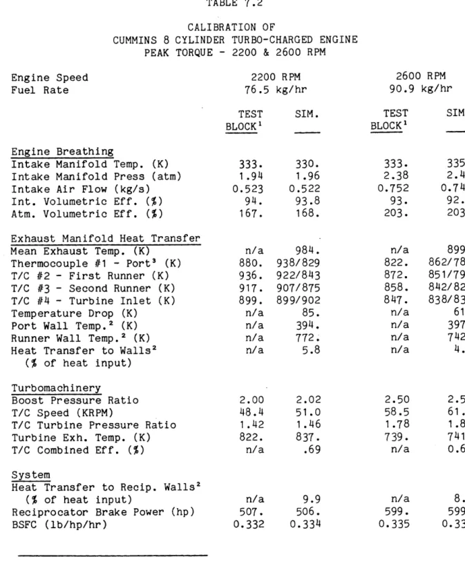
The port may contain either one or two exhaust valves. In either case only one control volume is used for what has been defined as the port. Figure 2.2 shows the layout of a typical head with two exhaust

valves per cylinder. In the case of an engine with two valves per

cylinder, the volume and surface area are calculated from the sum of the sections of the port before the exhaust streams come together and the common section downstream. The average cross-sectional area is weighted based on surface area of the individual sections and the surface area of the common section. Rush [1] found that changing the cross-sectional area of the port had almost no affect on the port heat transfer.

Apparently, the counter-balance between the increase in heat flux due to the higher gas velocities and the decrease in heat transfer surface area for a decrease in port flow area was such that the two effects cancelled each other out. The wall construction in terms of thickness and thermal properties is assumed to be the same for all parts of the port.

The heat transfer from the exhaust gases in the port to the exhaust valve(s) is not included in the port heat transfer. The reason for this omission is that the heat transfer to the exhaust valves from the port

is negligible with respect to the rest of the heat transfer to the port walls. In a normally cooled engine, the reason for the relatively low heat transfer to the valves is twofold. First, the exhaust valves represent less than 10% the inside surface area of the port. Second,

exhaust valve temperatures for diesel engines are typically 700-900K [10]. The port wall temperature for a water cooled engine is about 440-450K (this is substantiated by the results of this study). For port gas temperatures that are typically in the range of 800-900K, the

factor of three to four less than the temperature drop between the gases and the cooled port walls. For the same heat transfer coefficient, the effect of the smaller area and the lower temperature drop results in the heat transfer to the exhaust valves of 2.5 - 3% the heat transfer to the rest of the port. On an engine basis, the port heat transfer to the exhaust valves is even less significant. In an insulated engine, the valve heat transfer would be a higher percentage of the port heat transfer. However, because of the area ratio between the rest of the port and the exhaust valve(s) and the decreasing heat transfer due to insulation, the valve heat transfer in the port is assumed to be

negligible. The exhaust valves are implicitly included in the cylinder heat transfer as part of the cylinder head area.

CHAPTER 3.

MANIFOLD HEAT TRANSFER

The engine exhaust system is composed of the exhaust ports and the exhaust piping up to the inlet' of the turbocharger. The flow in this part of the engine is highly irregular with periods of very high mass flow and other periods of almost no mass flow. Consequently, the heat

transfer coefficient from the exhaust gases to the manifold wall varies substantially over the period of one cycle. Since the exhaust gases exit from the engine at temperatures ranging from 750 to 1000K and wall temperatures are as low as 400K, the heat transfer from the gases to the surroundings can be significant. In order to evaluate the heat transfer from the exhaust gases to the manifold walls, empirical heat transfer relations are applied. These relations are used in conjunction with the manifold thermal conductivity and the ambient boundary conditions are used to determine the heat transfer rate for the exhaust.

To determine the local heat transfer, the exhaust manifold is divided into sections connected in series. Each section is considered separately. Within each zone the gas temperature, the heat transfer coefficient, and the inside wall surface temperature are assumed to be uniform. Both the gas temperature and heat transfer coefficient are

allowed to vary with time. This model allows the inside wall surface temperature to be taken as either constant with time or varying with time. The method for the calculation of the wall temperature is the same as was developed by Assanis [11] for the cylinder heat transfer in the same program. Starting with an initial guess for the steady-state wall temperature, the new value for the wall temperature is calculated

at the end of each cycle based on the heat transfer over the previous cycle. Once the program heat transfer and mass flow have converged using steady-state wall temperatures, a transient calculation is done if it has been specified by the user. The transient solution is

superimposed on the steady-state solution to give the wall temperature profile as a function of time.

The heat transfer coefficient for the exhaust gases is determined using empirical correlations applied to the flow rate for each

particular section. For the port section, the results of Caton [71 are used. For the other sections of the manifold, turbulent pipe flow

correlations are used. The mass flow used in these correlations is the instantaneous average of the mass flow into and out of the section being analyzed.

3.1 Port Heat Transfer:

The heat transfer in the exhaust port is highly unsteady. When the exhaust valve first comes open, a high velocity jet of high temperature gases sets up recirculation zones in the port [5] that result in a higher heat transfer coefficient than the overall mass flow in the port

would indicate. When the exhaust valve is fully open, the flow resembles turbulent pipe flow and the heat transfer coefficient is related to pipe flow relationships. Then, as the exhaust valve closes, there is another period when a narrow jet of gases affects the heat transfer by again setting up recirculation zones. The period the valve closed is much longer than the period when it is open. During the closed period the mass flow rate approaches zero and a correspondingly low heat transfer coefficient exists.

In order to quantify the heat transfer in the exhaust port, the results of Caton [7] are applied. Based on experiments done with fast response fine wire temperature measurements of the port gas temperature

in a spark ignition engine, Caton arrived at the following correlations for the heat transfer for various phases of the exhaust process:

Valve opening phase ( L/D < 0.2 ):

(3-1

)

Nu = 0.4 Re.o.6

J

Valve open phase ( L/D > 0.2 ):

Nu = 0.023 CR CEE Re 0.8 Pr0.3 _(3-2)

Valve closing phase ( L/D

<

Nu = 0.5 Re.0.5

(3-3)

Valve closed phase:

Nu = 0.023 Re M Pr o4 _(3-4) D = valve diameter L = valve lift h D Nu = Nusselt Number = k

Re. = jet Reynolds Number =

V. = velocity of flow through v = dynamic viscosity of flow

V. D

x

V

exhaust valve where

V D Re = pipe Reynolds number =

V = pipe flow velocity

C = correction factor for surface roughness C = correction factor for entrance effects

EE

Two modifications were made to these results for the present study. The correction factor for surface roughness has not been included. The

effects of surface roughness on heat transfer and the reason for

excluding them in the present study are discussed in the next section. Also, during the period when the valve is closed, the mass flow is based

on the instantaneous mass flow rate between sections instead of on the average flow over the complete cycle as was done by Caton. For a turbocharged engine, this flow is not zero in general because gas flow is induced in inactive sections of the exhaust manifold by the pressure pulsations produced when other cylinders exhaust. Using the

instantaneous value of the mass flow rate throughout the cycle more closely approximates the process that actually occurs in an engine. It should be noted that this approach is not applicable to a naturally aspirated engine (such as Caton's) since in such engines the mass flow

during periods when the valve is closed approaches zero.

The correction factor for entrance effects, CEE, during the periods when the exhaust valve is fully open is the same as that used for the

other sections of the manifold and is discussed in the following section.

3.2 Other Sections of the Manifold:

For the other sections of the exhaust manifold downstream of the exhaust port, turbulent pipe flow correlations are applied. The heat transfer coefficient for fully developed flow in a straight pipe, can be found using the Dittus-Boelter equation [12]:

Nu = 0.023 Re' 8 Pr 0.3 (3-5)

In an exhaust manifold of an engine not all of the qualifying conditions for this equation apply. In general the flow is not fully developed and

the pipe is not straight. There are other factors as well that can cause a deviation from the heat transfer predicted by this equation. They are the variation of the gas properties with temperature, the

surface roughness, and viscous heating. For an accurate heat transfer model each of these possible factors should be considered and the base equation adjusted to account for their influence if it is necessary. Each of these effects was considered separately.

3.2.1 Entrance Effects

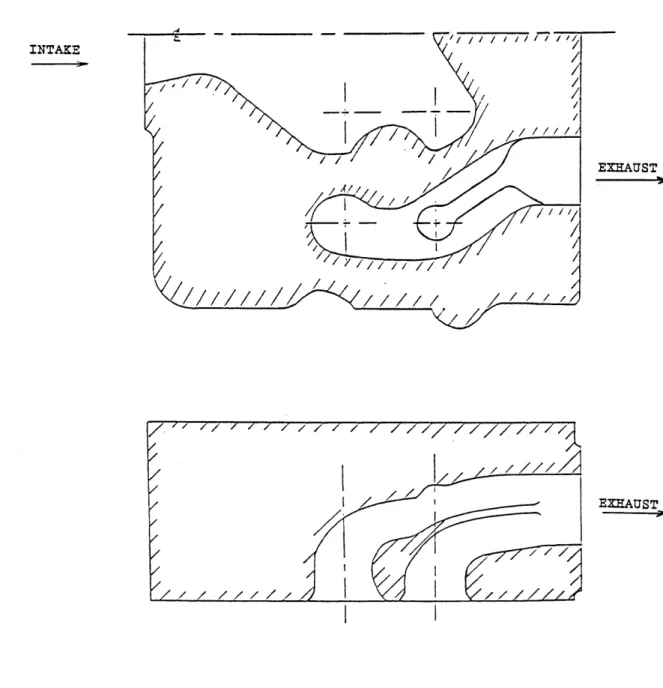
The heat transfer enhancement due to entrance effects was the subject of a study by Boelter, Young, and Iversen [13]. They did a series of experiments measuring the heat transfer coefficient under different flow conditions at a tube entrance. They found that the local heat transfer coefficient is raised by a factor of up to three at the

inlet of the tube. Both the magnitude of the intensification factor and rate at which it decays to unity were strongly dependent on the flow

characteristics at the tube entrance (e.g. fully developed velocity distribution vs. uniform velocity distribution, or a sharp bend at the

entrance vs. a straight pipe). Figure 3.1 shows some of their results. Fitting a curve to the experimental results for a tube with an elbow at the entrance, yields the following equation for the local heat transfer coefficient:

CEE~ Nu - 2.2 (x/D) -0.3 3 < x/D < 14 Nu

(3-6)

where x = entrance length from the inlet of the tube D = tube diameter

Nu = local Nusselt number x

Nu. = Nusselt number for fully developed flow

In order to find the average increase in heat transfer for a given section, equation 3-6 is integrated over the length of the section and

divided by its length.

L Nu 1 r2 CEE ave = f1 [2.2 (x/D) -0.3] dx EE 1Nu, L2- L L3 2 1 1 _(3-7) or, CL ) 0.7 07 (L ) '7- CL

)

where L = distance from the exhaust valve to the inlet of the section

L = distance from the exhaust valve to the outlet of the 2

section.

One disadvantage with using Boelter's results is that the experimental data was only taken up to Reynolds numbers of 55,000. In the engine exhaust, peak film Reynolds numbers of up to 400,000 are expected. Deissler [14,15] did analytical work that corresponded to Boelter's results but extended the range up to 200,000 and found that the influence of entrance effects was in general insensitive to Reynolds numbers effects. The insensitivity of the correlation to the Reynolds number and the relatively short time that the Reynolds number is above the range investigated justifies the use of the correlation for the exhaust flow.

3.2.2 Effect of Curved Pipe

A bend in a pipe with turbulent flow passing through it tends to increase the heat transfer coefficient from the fluid to the pipe wall because of a decrease in the boundary layer thickness in the vicinity of the bend. This effect tends to decrease as the Reynolds number and the overall level of turbulence increases. Hausen [16] recommends using the following correlation for the heat transfer enhancement due to bends in a tube:

Nu BP _0.141

C = =( 1 + 21 / Re ' d / D) (3-9)

BP _NuS

where C = correction factor for pipe bends NuBP Nusselt number for bent pipe Nu = Nusselt number for straight pipe

d = tube diameter D = bend diameter

This correlation has the advantage over other correlations given in the

literature [17,18,19] because it combines the results of the others to extend over a wide range of Reynolds numbers.

The bent pipe correlation is applied to the sections of the manifold

downstream of the port. In general, these sections may have both straight and bent portions. In order to account for bends without over compensating, the heat transfer enhancement due to a bend in a manifold section is weighted according to the percentage of the pipe section that is bent. In the code, the portion of the section that is bent is calculated from the radius of the bend and the total number of degrees of the bend in a given section. This approach in contrast to the results of Ede [20] who found that the heat

transfer coefficient is increased for some length downstream of the bend. However, he also found that the downstream length affected decreases with

increasing Reynolds number. In the range of Reynolds number for the exhaust manifold, the portion of the pipe affected downstream of the bend is

neglected.

3.2.3 Effect of Variable Gas Properties

With large temperature differentials between the bulk gas temperature and the wall temperature, the effect of the natural variation in the gas

properties can be a significant factor in the heat transfer calculations. Both the viscosity and the thermal conductivity of a gas vary with the temperature raised to the 0.68 power [15] and the density varies inversely with the temperature. The influence of temperature on these properties can affect the heat transfer when a large temperature drop exists between the gas bulk temperature and the wall temperature. The specific heat and the Prandtl number are not significantly affected by temperature.

There are two conflicting methods commonly used to account for the temperature dependence of these properties. One involves correcting the Nusselt number derived using bulk temperature properties. The correction factor is expressed as the ratio of the wall temperature to the bulk

temperature raised to a power. The exponent of the correction factor is determined by the geometry and the type of flow. The second method consists of evaluating the equations for heat transfer using the properties found at some reference temperature that accounts for the variation in such a way that the properties can be considered constant.

In order to use the first method, the appropriate exponent for the temperature ratio is needed. Experimental tests involving the cooling of gases under forced convection are rare but some evidence exists demonstrating

that for cooling of gases, the effect of property variation is nil for wall temperature to bulk temperature ratios greater than .25 [211. On this basis Kays and Perkins recommend that the exponent for the correction factor for property variation with temperature for heat extraction from gases should be

zero (ie. no correction is necessary).

The reference temperature method is used the most often to account for temperature dependent properties. In their analytical treatment, Deissler and Eian [14] recommend using a reference temperature based on a weighted average between the bulk and wall temperatures. For the cooling of gases, they found the following equation for the reference temperature:

T = 0.4 (T - Tb

)

T = bulk gas temperature

Most frequently however, the constant 0.4 in the above equation is changed to 0.5 to get what is called the film temperature.

There is an obvious difference between the two methods of correction that is not well explained in the literature. In the absence of a

definitive convention, the film temperature is used to evaluate the gas properties as this appears to be the most common practice.

3.2.4 Surface Roughness

If a surface is sufficiently rough, an increase in the heat transfer coefficient relative to that for a smooth surface can result. This increase is a function of both the surface roughness and the flow

Reynolds number. In general, for a given surface roughness, there is a minimum Reynolds number before an increase in the heat transfer

coefficient occurs. Heat transfer correlations for heat transfer

enhancement due to surface roughness are scarce. One common approach to account for this effect is to use the Colburn analogy [12] to relate the convective heat transfer coefficient to the fluid friction by the

following equation:

St Pr2/3 = f/2

Where St is the Stanton number defined as h/(pC V), Pr is the Prandtl number, and f is the flow friction factor. The increase in heat

transfer is thus related to the increase in the friction factor due to surface roughness. Reference to a Moody chart (see for ex'imple ref. 19) indicates that for the peak Reynolds numbers expected in the range of 300,000 to 400,000, the line for a relative roughness of 0.001 (based on a roughness of c=0.00015 ft) has just started to deviate from the

friction factor line for a smooth pipe. This indicates that there is some heat transfer enhancement due to surface roughness at the peak exhaust flows that occur during the blow down phase but that there is little increase in the heat transfer during the rest of the exhaust

process. Application of a correction factor for surface roughness is complicated by the need for a correlation to find the increase in friction factor as a function of surface roughness and Reynolds number and data for the appropriated values to be used for the surface

roughness of the inside of the exhaust manifold.

The correction used by Caton [7] for surface roughness was based on the results of Nunner. The correction factor in this case is also based on the increase in the flow friction factor relative to the friction factor for smooth pipe and is based on data up to flow Reynolds numbers of 80,000. It was not felt that this correlation would be appropriate for the present study.

Due to the marginal effect on convective heat transfer in the present application and the difficulty in applying an accurate

correlation, the heat transfer enhancement due to surface roughness was not included in this study. It should be noted that the heat transfer calculations that follow underestimate the heat transfer due to the omission of the surface roughness effects.

3.2.5 Viscous Heating

Viscous heating of the flow can result for flows of sufficiently high Mach number due to the shear forces between the fluid and the wall and the work done as the fluid moves against these forces. In order for viscous heating to be significant, the Mach number of the flow has to meet the following requirement :

M2 > 1 2.5 (3-11)

where M = Mach number

The maximum velocity in the exhaust manifold occurs during blow-down in the port. The engine simulation program for a representative engine gave a maximum flow rate in the port during this period of M = 0.5. On

the basis of this velocity it is seen that viscous heating effects can be neglected in determining the exhaust manifold heat transfer.

3.2.6 Summary

There are only two correction factors that are significant and need to be considered with respect to the heat transfer coefficient in the exhaust manifold. They are the enhancement of heat transfer due to the short length of pipe under consideration (entrance effects) and that due to pipe bends. Combining the formula for fully developed flow for a straight pipe with these correction factors gives the correlation used for the heat transfer coefficient for sections of the pipe downstream of the port section and for the exhaust port during the periods when the exhaust valve is fully open or closed:

Nu = 0.023 CEE CBP Re0.8 Pr0.3 (3-12)

3.3 Steady-State Heat Transfer Through a Composite Wall

In all of the heat transfer calculations for the exhaust manifold, the heat transfer from the gas to the walls is considered separately from the heat transfer from the walls to the environment. It is

expected that the simulation would normally would be run with the inside wall temperatures calculated based on the operating conditions of the engine. It will also accept specified inside wall temperatures.

For the predicted wall temperatures, the program must balance the two heat transfer rates averaged over a complete engine cycle. During the first cycles of a simulation, the program initially calculates the steady-state heat transfer through the manifold walls. The heat

transfer through the manifold wall is considered to be one-dimensional. The rate of heat transfer through the wall is found by:

Q = A U (T - T ) (3-13)

w c

where Q = heat transfer rate A = inside surface area

U = an overall heat transfer coefficient for the wall from the inside surface to the outside

Tw = the inside wall surface temperature

Tc = the outside (cold) surface temperature or cooling medium temperature.

Since low heat rejection engines can be expected to have manifold walls composed of layers of materials, the program is set up to accept up to accept three user defined layers each of a specified thickness and

thermal conductivity. The overall heat transfer coefficient, U, for a cylindrical composite wall is found from [191:

-1 ln (R2/ R ) ln (R3/ R2

(AU) = + + ... +

2 f L k 2

1 L kb 2, L R h (3-14)

where R = the inside radius of the inner layer of material 1

R3 = the outside radius of the second layer of material ka = the thermal conductivity of the inside layer of

material

kb = the thermal conductivity of the second layer of material

R = the outside radius of the wall

h = the outside heat transfer coefficient

The outside boundary condition must be specified by the user. It can be specified as either the outside surface temperature of the manifold wall or as an ambient temperature and heat transfer coefficient. In the case of specified outside wall temperatures, the last term in Equation 3-14

is dropped.

3.4 Determination of the Inside Wall Temperature

The inside wall surface temperature is calculated for each section of the exhaust manifold individually. Initially, whether the simulation

is being run with steady-state wall temperatures or as a transient wall temperature calculation, the wall temperature is held constant during a complete cycle iteration. Since the correct temperature is not known at the start of the simulation, initial guesses are used for the inside wall temperatures. Based on the results from each cycle, the wall

temperature is updated until convergence is achieved. Then, if transient wall temperature calculations are desired, the program

continues additional cycle iterations and calculates the transient wall temperatures until convergence is again reached. During the transient calculations, the constant, steady-state, wall temperatures are added to

the perturbed solution to find the temperature distribution in the walls as a function of time. Since the transient wall temperatures only

penetrate a very short distance into the wall [11], only a few cycles are required for the temperature profile to stabilize. The program is set up to run a minimum of two cycles for the transient temperature calculations to allow the temperature profiles in the wall to become established.

3.4.1 Steady-State Wall Temperature Determination

The method used for the wall temperature calculations was developed by Assanis [11] for use in the same program. The instantaneous heat

transfer rate to the walls is calculated from:

Qw (t) = h(t) (T (t) - Tw) (3-15)

where h(t) = instantaneous heat transfer coefficient

calculated as described in Sections 3.1 and 3.2

T = mean inside wall temperature (constant over the cycle)

T = the instantaneous gas temperature for the section

Based on the results from the previous cycle, an updated wall temperature can be found using the following equation:

h T + U T

Tg c (3-16)

w h +U

where the prime denotes the updated wall temperature to be used in the next cycle iteration. In order to carry out this calculation both the

heat transfer coefficient and the product of the heat transfer

coefficient and the gas temperature are integrated out over the complete cycle to find their time average values.

3.4.2 Transient Temperature Calculations

Transient wall temperature calculations are carried out by applying the Fourier equation in one dimension:

T 2T

3T a 2T _(3-17)

at

a

ax

This equation is applied using a finite difference analysis that calculates the wall temperature as a function of time throughout the cycle based on the heat transfer from the gas to the wall at that

instant. As discussed above, the transient temperature calculations are carried out after the steady-state solution has been found and the

results are superimposed to find the temperature profile. The development of the finite difference technique may be found in References 11 and 22.

There is a slight error introduced in the finite difference scheme applied to the exhaust manifold because the scheme is based on plane surface heat transfer while the exhaust manifold is cylindrical.

However, this error is negligible because the penetration depth of the transient temperature variations is small with respect to the inside radius of the exhaust manifold.

The heat transfer for the connecting pipe between the turbocharger and the power turbines is treated in the same way as for the exhaust manifold. The heat transfer coefficient is based on turbulent pipe flow using equation (3-12). The correction factor for the entrance effects

is calculated based on a new entrance to the pipe at the turbine exhaust. The wall thermal conductivity and the inside wall surface temperature are calculated in the same manner described in Sections 3.3 and 3.4.

PRESSURE LOSSES

The pressure drop for the exhaust manifold of a 6 cylinder diesel engine was found by Primus [6] to be a factor of 10 to 15 times higher than the pressure drop calculated based on the friction factor for

turbulent pipe flow. This increase in the flow losses is apparently due to the complex shape of the manifold and the interaction of the flow with the open passageways from other cylinders. For this reason, a specified flow loss factor is used for the calcul.ation of the exhaust manifold pressure drop. Thus, the pressure drop at any instant of time

is found from:

p = K (pV 2/2) (4-1)

where

p = pressure drop in Pascals

V = instantaneous velocity in the manifold p = manifold density

The velocity of the flow used in the pressure drop calculation for the exhaust manifold is based on the instantaneous mass flow through the turbine and the cross sectional area of the first runner. Similarly, the velocity of the flow for the connecting pipe between the turbines is based on the average turbine mass flow and the cross sectional area of the turbine connecting pipe.

Primus found that suitable values for K for the exhaust manifold were between 2 and 3.5. However, in the present study loss coefficients in this range gave an excessive pressure drop through the exhaust

manifold. Values of K between 0.5 and 1.0 gave more reasonable results in the current investigation.

There are two reasons for the difference between the two flow loss factors. The first is the fact that in the present study the turbine inlet flow was used to determine the flow velocity. The turbine inlet flow is in general higher than the mass flow through a runner and a pressure drop calculation based on this value will yield a higher result. The second is the sensitivity of the pressure drop to the manifold diameter used for the calculation. For a constant mass flow,

the pressure drop varies with the diameter of the manifold raised to the fourth power. A slight difference in the diameter used for the

representative section when calculating the pressure drop could easily explain the difference in flow loss factor between the two studies. A flow loss factor of 0.5 was used for the exhaust manifold in all of the

CHAPTER 5. THERMODYNAMIC EQUATIONS

5.1 General Equations

The three main control volumes of interest in the program are the intake manifold, the master cylinder, and the exhaust manifold. For each of these components the program determines the Thermodynamic State of the gases by integrating the derivatives with respect to time of the temperature, mass, pressure, and fuel fraction. The time derivatives for these properties are determined from the following equations based on the conservation of mass, conservation of fuel mass, the ideal gas law, and the First Law of Thermodynamics [11 ,22]:

Change in Mass with respect to time:

m = I m. (5-1)

Change in Fuel Fraction with respect to time:

F = E m.F. - mF (5-2)

Change in Temperature with respect to time:

T = 1(1- V C + -(z m.h. Q B V B Bm h J w (5-3) where A = c + - - c

)

CP

1 F (F/A) ti 0 (1- F)

Change in Pressure with respect to time:

P = -- _ _ V 1 ap * 32 + n 3p/ p .V p 5T T P 3 m

(5-4)

The exhaust manifold is further broken down into smaller sub-control volumes that are contained within the manifold control volume (see

Chapter 2). For these sub-control volumes, the pressure derivative is that which is determined for the average exhaust manifold based on equation 5-4. With the pressure derivative an independent variable determined for the average manifold, the mass derivatives for the sub-control volumes become dependent variables. Rearranging equation (5-4) gives: m .

v

[

where the subscript i refers to the different sub-control volumes of the exhaust manifold.

By applying equations (5-1),(5-2),(5-3), and (5-5) to each separate sub-control volume of the manifold, the properties of each section can be determined.

The mass flow between sections of the exhaust manifold is determined by the mass flow rate through the exhaust valve and the rate of mass storage (i.e. retention) within any sections upstream of the section in question due to changes in the properties of those sections. Thus, the

mass flow out of the port section and into the runner section is found by subtracting the change in mass in the port as found by equation (5-5) from the mass flow through the exhaust valve.

5.2 Solution of the Equations

The solution of the simultaneous equations that result for the exhaust manifold is obtained through an iterative procedure. A Gauss-Seidel scheme is used that repeats the calculation of the derivatives for the exhaust manifold until convergence is achieved [291. For the

initial guess for the unknown time derivatives, the values from the previous call to the subroutine is used. The convergence of the new values for the derivatives is checked using Euclidean norms via the following equation:

U(s+1) _{- " |}

(s+ 1< (5-6)

IN

lU l

112

where U = the new value of manifold derivatives U = the old value of the manifold derivatives c = the error tolerance

The Euclidean norm is defined by:

iU~

i=1

The proper error tolerance, c, was found by doing a series of runs with different values of c. For large values of e the simulation ran longer because extra cycles were required for the program to converge. With small values of e run times increased because extra loops were made through the exhaust manifold iteration. A minimum run time was observed

value for e was determined in this manner to be 5x10-5

In this application the iterative procedure has certain advantages over direct methods (e.g. Gauss elimination) for the solution of the set of simultaneous equations for the exhaust manifold. First, it is more flexible. The program accepts the total number of control volumes to be used for the exhaust manifold as an input parameter. Given the

complexity of the equations for the exhaust manifold, building in the same flexibility for a direct solution would have been considerably more difficult. Second, the resulting program is easier to follow for

someone unfamiliar with the code. With the iterative procedure, it is not necessary to set up the actual matrix. The equations appear in the program essentially as they are written above. Finally, the computation

time for the iterative solution is competitive with direct solution procedures. Since the program progresses in small steps, the new values for the derivatives are not changed much from the old values and

convergence is reached rapidly. On the average, the loop for the

exhaust manifold derivatives is passed through 1.5 times per call to the subroutine where they are calculated. The average number of passes

through the loop is less than two because the predictor-corrector scheme of the integration routine often results in the exhaust manifold

derivatives being calculated twice with only slightly different sets of conditions. For these calls to the subroutine for the exhaust manifold derivatives, the change in the values for the derivatives is not large enough to exceed the convergence tolerance and the loop is not repeated.