Science Arts & Métiers (SAM)

(1)

Science Arts & Métiers (SAM)

is an open access repository that collects the work of Arts et Métiers Institute of Technology researchers and makes it freely available over the web where possible.

This is an author-deposited version published in: https://sam.ensam.eu Handle ID: .http://hdl.handle.net/10985/21897

To cite this version :

Luca SCIACOVELLI, Donatella PASSIATORE, Paola CINELLA, Pascazio GIUSEPPE -

Assessment of a high-order shock-capturing central-difference scheme for hypersonic turbulent flow simulations - Computers and Fluids - Vol. 230, p.105134 - 2021

Any correspondence concerning this service should be sent to the repository

Administrator : [email protected]

(2)

Assessment of a high-order shock-capturing central-difference scheme for hypersonic turbulent flow simulations

Luca Sciacovelli

^a^,∗

, Donatella Passiatore

^a^,^b

, Paola Cinnella

^a

, Giuseppe Pascazio

^b

aArts et Métiers ParisTech, DynFluid Laboratory, 75013 Paris, France

bPolitecnico di Bari, DMMM, 70125 Bari, Italy

A B S T R A C T

High-speed turbulent flows are encountered in most space-related applications (including exploration, tourism and defense fields) and represent a subject of growing interest in the last decades. A major challenge in performing high-fidelity simulations of such flows resides in the stringent requirements for the numerical schemes to be used. These must be robust enough to handle strong, unsteady discontinuities, while ensuring low amounts of intrinsic dissipation in smooth flow regions. Furthermore, the wide range of temporal and spatial active scales leads to concurrent needs for numerical stabilization and accurate representation of the smallest resolved flow scales in cases of under-resolved configurations. In this paper, we present a finite-difference high-order shock-capturing technique based on Jameson’s artificial diffusivity methodology. The resulting scheme is ninth-order-accurate far from discontinuities and relies on the addition of artificial dissipation close to large gradient flow regions. The shock detector is slightly revised to enhance its selectivity and avoid spurious activations of the shock-capturing term. A suite of test cases ranging from 1D to 3D configurations (namely, perfect-gas and chemically reacting shock tubes, Shu–Osher problem, isentropic vortex advection, under-expanded jet, compressible Taylor–Green Vortex, supersonic and hypersonic turbulent boundary layers) is analyzed in order to test the capability of the proposed numerical strategy to handle a large variety of problems, ranging from calorically-perfect air to multi-species reactive flows. Results obtained on under- resolved grids are also considered to test the applicability of the proposed strategy in the context of implicit Large-Eddy Simulations.

1. Introduction

Hypersonic flight has gained renewed attention in recent years, due to its importance for multiple breakthrough applications in the defense and military fields, as well as in the areas of spatial tourism and trans-atmospheric flight [1]. The accurate prediction of hypersonic flow fields is a challenging task, due to the massive conversion of kinetic energy from the hypersonic free stream into internal energy as the fluid approaches the body. The shock waves generated in such flight conditions produce a sharp increase in the fluid temperature, possibly causing vibrational excitation and gas dissociation, and resulting in a nonequilibrium thermochemical state. These processes have major effects on aerodynamic performance, heat transfer rates, fluid-surface interaction (e.g., ablation), and hydrodynamic instabilities leading to boundary layer transition and breakdown to turbulence [2]. Their accurate prediction is of crucial importance for the design of the thermal protection system and the prediction of the overall force and heat transfer coefficients, and requires advanced numerical solvers

and models. In this paper, the focus is put on so-called high-fidelity numerical schemes for Direct Numerical Simulation (DNS) and Large Eddy Simulation (LES), two major enablers for a deeper understanding of out-of-equilibrium flow regions dominated by laminar-to-turbulent transition and turbulent regimes.

A major difficulty in DNS and LES of high-speed flows is the extreme sensitivity of small flow scales to numerical approximation errors. The occurrence of shock waves, with physical thicknesses of the order of a few mean free paths, leads to unfeasible resolution requirements for numerical simulations, at least in the strict DNS sense. On the other hand, velocity fluctuations of the order of the sound speed [3]

may lead to the formation of eddy shocklets, embedded in the turbulent flow. Usually, both kinds of structures are dealt with by using shock-capturing techniques. These consist in locally injecting controlled amounts of numerical dissipation to spread shocks over a few mesh cells wherever the mesh is not sufficiently fine to resolve the shock thickness. This technique, corresponding to a regularization method,

(3)

contrasts with the need of using low-dissipation schemes not to alter the fine-scale turbulent motions. These opposite requirements become even more critical as the Mach and Reynolds numbers increase, because of the growing difficulty to distinguish strong gradients due to shocks from those related to turbulent fluctuations. In such a challenging framework, much effort has been done to devise numerical methods able to handle strong shock waves, while ensuring minimal amounts of dissipation elsewhere.

Two great families of discretization method for the non-linear terms in the Euler and Navier–Stokes equations can be distinguished [4]: the first one, originally designed to handle inviscid flows with strong discontinuities, relies on some form of upwinding along with flux or slope limiters ensuring non-linear stability; the second one – in principle more suited for smooth flows – uses central schemes supplemented with some form of filtering or artificial dissipation or, alternatively, ensuring discrete conservation of solution invariants such as the overall kinetic energy. Despite the large number of comparative studies [5–7], a global consensus on the ‘‘best’’ numerical strategy for high-speed turbulent flows has not been reached, since each method proposes a different compromise among concurrent needs: namely, high accuracy, robustness, low computational cost, few tuning parameters and suitability for different configurations.

A well-known drawback of the first class of schemes is the excess of numerical viscosity introduced in the solution, leading to spurious entropy generation and kinetic energy losses in the low Mach number limit [8]. Weighted essentially non-oscillatory (WENO) schemes are probably the most popular upwind schemes in the context of LES and DNS of compressible flows. First introduced by Liu et al. [9] and later improved by Jiang & Shu [10], they rely on the assembly of high-order numerical fluxes from linear combination of lower-order polynomial reconstructions using suitable weighting coefficients. Many variants have been proposed, e.g., to improve their dispersion and dissipation properties [11,12] and to reduce the nonlinear dissipation [13,14]. Coupling with purely central schemes has led to hybrid methods [15,16] and enhanced weighting strategies and smoothness sensors [17–20]. Contrary-wise, the family of central schemes generally introduces very low dissipation, provided that a selective enough numerical filter or artificial viscosity term is used, but is generally limited to compressible flows at moderately supersonic Mach numbers, i.e. with weak shocks. These schemes must be supplemented with selective nonlinear filtering [21–24], artificial diffusive fluxes [21,25,26], or localized artificial diffusivity (LAD) under the form of modified transport coefficients [27–29] for damping grid-to-grid oscillations in smooth flow regions and to ensure shock capturing. The amount of numerical dissipation introduced at a point of the computational domain is adjusted by means of properly-devised sensors, allowing to switch on shock-capturing capabilities where needed. Shock-capturing high- order central-difference schemes have been successfully applied, for instance, to overexpanded jet flows with shock cells [30] and high- speed boundary layers of perfect gases up to Mach 6 [31], as well as to the direct and large-eddy simulations of high-speed flows of single- species, molecularly complex gases at thermodynamic conditions close to the liquid/vapor critical point up to Mach 6 [32–35]. However, their suitability for the numerical simulation of severe hypersonic, chemically reacting flows with strong shocks and stiff chemical reactions has not yet been assessed.

For LES, where only the dynamics of the large scales is computed while the effects of sub-grid scales (SGS) are modeled, the choice of the numerical scheme is possibly even more critical than in DNS. Scale sep- aration is indeed difficult to establish since the cut-off between resolved and modeled scales is not sharp and arises from a complex combination of implicit filtering by the grid and the discretization schemes.

The intricate interactions between numerical errors and SGS modeling errors has been investigated by numerous authors (a recent discussion can be found in [36]), leading once again to two separate modeling strategies: one relying on the explicit introduction of a SGS model, and

the other one using the dissipative part of the discretization scheme for ensuring regularization of the unresolved SGS scales [37–41]. The latter has become increasingly spread in the scientific community, due to the good tradeoff between computational cost and accuracy offered for a wide range of applications, provided that a high-resolution scheme is used along with sufficiently resolved computational grids [36,42].

The goal of the present study is twofold: (i) to assess the capability of a high-order shock-capturing central scheme, used in our previous works [32,35], to robustly predict compressible flows with shock waves and chemical nonequilibrium effects while accurately resolving fine-scale turbulent structures; and (ii) to demonstrate the suitability of the non-linear numerical dissipation of the scheme to act as a SGS regularization in under-resolved turbulent flow simulations.

The scheme uses tenth-order accurate finite-difference approximations of the non-linear fluxes, supplemented with a higher-order extension of Jameson’s adaptive artificial dissipation [25]. The order of accuracy of the artificial viscosity term is chosen to obtain an overall dissipative-dominant truncation error, which reduces the appearance and amplification of spurious oscillations [43] and limits the activation of lower-order nonlinear viscosity. The latter is triggered by a highly- selective shock sensor, built on a combination of the original Ducros’

extension [44] of Jameson’s pressure-based sensor with the Bhagatwala

& Lele [45] modification proposed in the context of LAD methods (more details are given in Section3). The scheme is applied to a suite of well- documented test cases of increasing complexity, ranging from 1D and 2D inviscid flow problems to the 3D simulation of a fully turbulent boundary layer at Mach 10 in chemical nonequilibrium conditions. The results are systematically assessed against exact or numerical reference solutions.

The paper is structured as follows. Section2reports the governing equations under investigation, along with the models used for thermodynamics, transport properties and chemical source terms. The high-order shock-capturing scheme is presented in Section 3. Sec- tions4and5contain a selection of preliminary validation cases and multi-dimensional turbulent configurations, respectively. Conclusions are drawn in Section6.

2. Governing equations

Our goal is to simulate flows governed by the compressible Navier–

Stokes equations for multicomponent chemically-reacting gases, written in differential form:

𝜕𝜌

𝜕𝑡+(𝜕𝜌𝑢_𝑗)

𝜕𝑥_𝑗 = 0 (1)

𝜕(𝜌𝑢_𝑖)

𝜕𝑡 +𝜕(

𝜌𝑢_𝑖𝑢_𝑗+𝑝𝛿_𝑖𝑗)

𝜕𝑥_𝑗 =𝜕𝜏_𝑖𝑗

𝜕𝑥_𝑗 (2)

𝜕(𝜌𝐸)

𝜕𝑡 +𝜕[

(𝜌𝐸+𝑝)𝑢_𝑗]

𝜕𝑥_𝑗 =𝜕(𝑢_𝑖𝜏_𝑖𝑗−𝑞_𝑗)

𝜕𝑥_𝑗 − 𝜕

𝜕𝑥_𝑗 (_NS

∑

𝑛=1

𝜌_𝑛𝑢^𝐷

𝑛𝑗ℎ_𝑛 )

(3)

𝜕𝜌_𝑛

𝜕𝑡 +𝜕( 𝜌_𝑛𝑢_𝑗)

𝜕𝑥_𝑗 = −

𝜕𝜌_𝑛𝑢^𝐷_𝑛𝑗

𝜕𝑥_𝑗 +𝜔̇_𝑛 (𝑛= 1,…,NS− 1) (4) In the preceding equations, 𝜌_𝑛 is the density of the 𝑛th species, 𝜌=∑NS

𝑛=1𝜌_𝑛the mixture density, NS the total number of species,𝑢_𝑖the velocity vector components in a Cartesian coordinate system, 𝑝 the pressure, 𝛿_𝑖𝑗 the Kronecker symbol and 𝜏_𝑖𝑗 the viscous stress tensor.

In Eq.(3),𝐸=𝑒+¹₂𝑢_𝑖𝑢_𝑖represents the specific total energy (with𝑒the mixture specific internal energy) and𝑞_𝑗 the heat flux; moreover,𝑢^𝐷_𝑛𝑗, ℎ_𝑛, and𝜔̇_𝑛 denote the𝑛th species diffusion velocity, specific enthalpy and rate of production, respectively. For temperature values lower than 9000 K, ionization and electronic processes can be usually neglected;

air is then modeled as a five-species mixture of N₂, O₂, NO, O and N (NS = 5[46]). To ensure total mass conservation, we solve for the mixture density and NS−1 species conservation equations, the NS-th species being computed as𝜌_NS=𝜌−∑NS−1

𝑛=1 𝜌_𝑛. This species is chosen

(4)

to be Nitrogen since it is the most abundant species (i.e., having the largest mass fraction) throughout the computational domain for each case. The viscous stress tensor is modeled as:

𝜏_𝑖𝑗=𝜇 (𝜕𝑢_𝑖

𝜕𝑥_𝑗 +𝜕𝑢_𝑗

𝜕𝑥_𝑖 )

−2 3𝜇𝜕𝑢_𝑘

𝜕𝑥_𝑘𝛿_𝑖𝑗, (5)

with 𝜇 the mixture dynamic viscosity. The heat flux is modeled by means of Fourier’s law, 𝑞_𝑗 = −𝜆^𝜕𝑇

𝜕𝑥𝑗, 𝜆 being the mixture thermal conductivity and𝑇the temperature. Each species is assumed to behave as a perfect gas; Dalton’s pressure mixing law leads then to the thermal equation of state:

𝑝=

∑NS

𝑛=1

𝑝_𝑛=𝜌𝑇

∑NS

𝑛=1

𝑌_𝑛

𝑛

=𝑇

∑NS

𝑛=1

𝜌_𝑛𝑅_𝑛, (6)

𝑌_𝑛 = 𝜌_𝑛∕𝜌, 𝑅_𝑛 and𝑛 being the mass fraction, gas constant and molecular weight of the 𝑛th species, respectively, and  = 8.314 J/mol K the universal gas constant. The thermodynamic properties of high-𝑇 air species are computed considering the contributions of translational, rotational and vibrational modes (named TRV formula- tion [47]); specifically, the internal energy reads:

𝑒=

∑NS

𝑛=1

𝑌_𝑛ℎ_𝑛−𝑝

𝜌, with ℎ_𝑛=ℎ⁰_{𝑓 ,𝑛}+

∫

𝑇 𝑇_ref

(𝑐^tr_𝑝,𝑛+𝑐_𝑝,𝑛^rot)d𝑇^′+𝑒^vib_𝑛 . (7) Here,ℎ⁰

𝑓 ,𝑛is the𝑛th species enthalpy of formation at the reference temperature (𝑇_ref= 298.15 K),𝑐_𝑝,𝑛^tr and𝑐^rot_𝑝,𝑛 the translational and rotational contributions to the isobaric heat capacity of the𝑛th species, computed as

𝑐^tr

𝑝,𝑛= 5

2𝑅_𝑛 and 𝑐^rot

𝑝,𝑛=

{𝑅_𝑛 for diatomic species

0 for monoatomic species, (8) and𝑒^vib

𝑛 the vibrational energy of species𝑛, given by 𝑒^vib_𝑛 = 𝜃_𝑛𝑅_𝑛

exp (𝜃_𝑛∕𝑇) − 1, (9)

with 𝜃_𝑛 the characteristic vibrational temperature of each molecule (3393 K, 2273 K and 2739 K for N₂, O₂ and NO, respectively [46]).

After the numerical integration of the conservation equations, temperature is computed from the specific internal energy by means of Newton–Raphson iterations.

Pure species’ viscosity and thermal conductivities are computed using curve-fits by Blottner et al. [48] and Eucken’s relations [49]:

𝜇_𝑛= 0.1 exp[(𝐴_𝑛ln𝑇+𝐵_𝑛) ln𝑇+𝐶_𝑛], 𝜆_𝑛=𝜇_𝑛 (5

2𝑐_𝑣,𝑛^tr +𝑐^rot_𝑣,𝑛+𝑐_𝑣,𝑛^vib )

(10) where𝐴_𝑛,𝐵_𝑛and𝐶_𝑛are fitted parameters. The corresponding mixture properties are evaluated by means of Wilke’s mixing rules [50]:

𝜇=

∑NS

𝑛=1

𝑋_𝑛𝜇_𝑛

∑NS 𝑚=1𝑋_𝑚𝜙_𝑛𝑚

, 𝜆=

∑NS

𝑛=1

𝑋_𝑛𝜆_𝑛

∑NS 𝑚=1𝑋_𝑚𝜙_𝑛𝑚

(11)

where𝑋_𝑛= 𝑌_𝑛𝑅_𝑛

∑NS 𝑚=1𝑌_𝑚𝑅_𝑚

denotes the molar fraction of species𝑛and

𝜙_𝑛𝑚= 1

√8 (

1 +𝑛

𝑚

)−¹ 2⎡

⎢⎢

⎣ 1 +

(𝜇_𝑛 𝜇_𝑚

)−¹ 2(𝑚

𝑛

)¹₄⎤

⎥⎥

⎦

2

. (12)

Mass diffusion is modeled by means of Fick’s law:

𝜌_𝑛𝑢^𝐷_𝑛𝑗= −𝜌𝐷_𝑛𝜕𝑌_𝑛

𝜕𝑥_𝑗 +𝜌_𝑛

∑NS

𝑛=1

𝐷_𝑛𝜕𝑌_𝑛

𝜕𝑥_𝑗, (13)

where the first term on the r.h.s. represents the effective diffusion velocity and the second one is a mass corrector term that should be taken into account in order to satisfy the continuity equation when dealing with non-constant species diffusion coefficients [51,52]. Specifically, 𝐷_𝑛is an equivalent diffusion coefficient of species𝑛into the mixture,

computed following Hirschfelder’s approximation [53] as 𝐷_𝑛= 1 −𝑌_𝑛

∑NS 𝑚=1 𝑚≠𝑛

𝑋_𝑛 𝐷_𝑚𝑛

with 𝐷_𝑚𝑛=1

𝑝exp (𝐴_4,𝑚𝑛)𝑇^[^𝐴^1,𝑚𝑛^(ln𝑇⁾²^+𝐴^2,𝑚𝑛^ln^𝑇+𝐴^3,𝑚𝑛^]

(14) where𝐷_𝑚𝑛is the binary diffusion coefficient of species𝑚into species𝑛, and𝐴_1,𝑚𝑛,…, 𝐴_4,𝑚𝑛are curve-fitted coefficients computed as in Gupta et al. [54].

The five species interact with each other through a reaction mech- anism consisting of five reversible chemical steps, according to Park’s model [46,55]:

R1∶ N₂+M ⟺2N+M R2∶ O₂+M ⟺2O+M

R3∶ NO+M⟺N+O+M (15)

R4∶ N₂+O ⟺NO+N R5∶ NO+O⟺N+O₂

being M the third body (any of the five species considered). Dissociation and recombination processes are described by reactions R1, R2 and R3; whereas the shuffle reactions R4 and R5 represent rearrangement processes. The mass rate of production of the𝑛th species is governed by the law of mass action:

̇ 𝜔_𝑛=𝑛

∑NR

𝑟=1

(𝜈^′′_𝑛𝑟−𝜈_𝑛𝑟^′)

× [

𝑘_{𝑓 ,𝑟}

∏NS

𝑛=1

(𝜌𝑌_𝑛

𝑛

)𝜈^′_𝑛𝑟

−𝑘_𝑏,𝑟

∏NS

𝑛=1

(𝜌𝑌_𝑛

𝑛

)𝜈^′′_𝑛𝑟] , (16) where𝜈^′

𝑛𝑟 and𝜈^′′

𝑛𝑟are the stoichiometric coefficients for reactants and products in the 𝑟th reaction for the 𝑛th species, respectively, and NR is the total number of reactions. Lastly,𝑘_{𝑓 ,𝑟} and𝑘_𝑏,𝑟 denote the forward and backward reaction rates of reaction𝑟, modeled by means of Arrhenius’ law.

For configurations in which air is modeled as a single-species calorically-perfect gas, a constant specific heat ratio is considered (𝛾 = 1.4), such that 𝑐_𝑝 = 𝛾𝑅

𝛾− 1. Since NS = 1 and there is no chemical activity, Eq.(4)is not solved and the diffusion velocity is zero.

Unless otherwise stated, viscosity is computed by means of Sutherland’s Law,𝜇(𝑇) = 𝐶𝑇^3∕2

𝑇+𝑆, with𝐶 = 1.457933 × 10⁻⁶kg∕m s K^1∕2 and𝑆 = 110.4 K, whereas the thermal conductivity follows a constant-Prandtl assumption, for which𝜆=Pr∕(𝜇𝑐_𝑝).

3. Numerical method

In this section we describe the high-order shock-capturing central- difference numerical scheme under investigation. We first present the most important ingredient, i.e. the spatial discretization scheme for the nonlinear terms, for a 1D system of hyperbolic conservation laws:

𝜕𝑤

𝜕𝑡 +𝜕𝑓(𝑤)

𝜕𝑥 = 0 (17)

where 𝑤 is the vector of conservative variables and 𝑓(𝑤) the flux function, such that𝐴 = 𝜕𝑓∕𝜕𝑤is a diagonalizable matrix with real eigenvalues. Extension to multidimensional cases is straightforwardly carried out by applying the scheme in each direction. Introducing the classical difference and cell-average operators over one cell:

(𝛿∙)_𝑗∶= (∙)_𝑗+1 2

− (∙)_𝑗−1 2

, (𝜇∙)_𝑗+1 2

∶=1 2

[(∙)_𝑗+1+ (∙)_𝑗]

(18) and considering a regular Cartesian grid with constant mesh spacing 𝛿𝑥(so that𝑥_𝑗=𝑗 𝛿𝑥), a conservative semi-discrete approximation of the spatial derivative writes:

(𝜕𝑤

𝜕𝑡 )

𝑗+(𝛿)𝑗

𝛿𝑥 = 0 (19)

(5)

The numerical flux at cell interface𝑗+¹

2,_𝑗+¹

2

, can be calculated using a simple upwind scheme, written hereafter as the sum of a central approximationand a dissipative term[56]:

_𝑗+¹

2

=_𝑗+¹

2

−_𝑗+¹

2

(20)

_𝑗+¹

2

=𝑓_𝑗₊₁+𝑓_𝑗 2 = (𝜇𝑓)

𝑗+¹₂ (21)

_𝑗+1 2

=1 2|𝑄

𝑗+¹₂|(𝑤_𝑗+1−𝑤_𝑗) = 1

2(|𝑄|𝛿𝑤)_𝑗+1 2

(22) with𝑄 a dissipation matrix. For instance,𝑄= ¹

2𝐼 (with 𝐼the iden- tity matrix) gives Lax–Friedrichs’ scheme [57],𝑄 = 𝜌(𝐴)𝐼 Rusanov’s scheme [58] (𝜌(𝐴)being the spectral radius of the flux Jacobian matrix 𝐴), and 𝑄 = 𝐴_𝑅 Roe’s scheme [59] (with𝐴_𝑅 the Roe matrix). All such schemes are monotonicity preserving according to Godunov’s the- orem [60], but only first-order-accurate, which makes them unsuitable for turbulence resolving simulations.

A standard way for increasing accuracy consists in using MUSCL extrapolations [61]. Here we adopt an alternative approach, first introduced in [56] to construct a third-order scheme and generalized to any order of accuracy in [62], which consists in recursively correcting the truncation error of Eqs.(21),(22). For a scheme of order2𝑃+ 3with a stencil of2(𝑃+ 2) + 1points, the numerical flux is of the form:

_𝑗+1 2

= [(

𝐼−

∑𝑃 𝑝=0

𝑎_𝑝𝛿^2+2𝑝 )

𝜇𝑓 − 𝑎_𝑃

2|𝑄|𝛿^2𝑃⁺³𝑤 ]

𝑗+¹₂

(23)

The coefficients 𝑎_𝑝 have alternate negative and positive signs as 𝑃 increases. The interested reader may refer to [62] for details about their calculation.

The preceding high-order, constant coefficient schemes are not total variation diminishing (TVD) nor monotonicity preserving, and slope or flux limiters should be introduced to avoid the appearance of spurious oscillations. Note that only schemes of odd order accuracy are included in the family, with a leading truncation error term given by:

𝜀= 𝑎_𝑃

2𝛿𝑥^2𝑃⁺³𝜕^2(𝑃⁺²⁾𝑤

𝜕𝑥^2(𝑃⁺²⁾ (24)

proportional to an even-order derivative, i.e. of dissipative nature.

Explicit odd-order schemes with constant coefficients have been shown to remain stable in the maximum norm𝐿_∞under the CFL constraint for problems with non-smooth initial conditions [43,63]. This implies that, although the considered schemes do generate spurious oscillations around discontinuities, such oscillations remain bounded in space and time. For the sake of clarity, we give hereafter the expressions of the schemes of order 3 to 9 (i.e.𝑃= 0,1,2and 3) of the preceding family:

_𝑗+¹

2

=[(

𝐼−1 6𝛿²)

𝜇𝑓 + 1 12|𝑄|𝛿³𝑤]

𝑗+¹ 2

(order 3) (25)

_𝑗+¹

2

=[(

𝐼−1 6𝛿²+ 1

30𝛿⁴ )

𝜇𝑓 − 1 60|𝑄|𝛿⁵𝑤

]

𝑗+¹ 2

(order 5) (26)

_𝑗+¹

2

=[(

𝐼−1 6𝛿²+ 1

30𝛿⁴− 1 140𝛿⁶)

𝜇𝑓 + 1

280|𝑄|𝛿⁷𝑤]

𝑗+¹ 2

(order 7) (27)

_𝑗+1 2

=[(

𝐼−1 6𝛿²+ 1

30𝛿⁴− 1 140𝛿⁶+ 1

630𝛿⁸)

𝜇𝑓 − 1

1260|𝑄|𝛿⁹𝑤]

𝑗+¹₂

(order 9) (28)

The same schemes can be derived in the finite volume framework by applying MUSCL reconstruction to the physical fluxes [62]. Specifically, for𝑄=𝐴_𝑅, one recovers a flux-extrapolation higher-order extension of Roe’s scheme. This choice has the advantage of introducing the minimal amount of numerical damping along each characteristic field. However, the extension of Roe’s average to real-gas flows is not unique and can introduce significant overcost (see, e.g. [64,65]).

With the purpose of simplifying the application to real-gas flows and reducing computational cost, a different approach is adopted. We

first observe that the preceding schemes can be considered as standard central-difference approximations of order 2(𝑃 + 2) on 2(𝑃 + 2) + 1 points of the flux derivative, plus a high-order artificial viscosity of order2𝑃+ 3on the same stencil depending on matrix𝑄. Afterwards, we choose𝑄=𝜌(𝐴), as in Rusanov’s scheme, which is less optimal than Roe’s matrix but avoids complexities associated with the extension of the approximate Riemann solver to real gases. This leads to a scalar numerical dissipation term of the form:

_𝑗₊¹

2

=[𝑎_𝑃

2𝜌(𝐴)𝛿^2𝑃⁺³𝑤]

𝑗+¹₂ (29)

Finally, we nonlinearly combine the preceding high-order dissipation with a lower-order term activated in the vicinity of flow discontinuities by means of a highly selective shock sensor. The dissipationthen becomes:

_𝑗₊¹

2

=𝜌(𝐴)

𝑗+¹₂

[𝜀₂𝛿𝑤+ (−1)^(𝑃+1)𝜀_2(𝑃₊₂₎𝛿^(2𝑃+3)𝑤]

𝑗+¹₂ (30)

with 𝜀₂

𝑗+¹ 2

=𝑘₂max(𝜑_𝑗, 𝜑_𝑗+1), 𝜀_2(𝑃₊₂₎

𝑗+¹ 2

= max(0, 𝑘_2(𝑃₊₂₎−𝑘_𝜀𝜀₂

𝑗+¹ 2

),

(31) where𝑘₂ and𝑘_2(𝑃₊₂₎are adjustable dissipation coefficients and𝑘_𝜀 is a constant equal to𝑎₀∕𝑎_𝑃, determining the threshold below which the higher-order dissipation is switched off.

For schemes of order 3 to 9, this gives the following expressions:

𝑗+¹₂ =𝜌(𝐴)_𝑗+1 2

[𝜀₂𝛿𝑤−𝜀₄𝛿³𝑤]

𝑗+¹₂ 𝜀_4𝑗+1 2

= max(0, 𝑘₄−𝜀_2𝑗+1 2

) (32)

_𝑗+¹

2

=𝜌(𝐴)_𝑗+1 2

[𝜀₂𝛿𝑤+𝜀₆𝛿⁵𝑤]

𝑗+¹

2

𝜀_6𝑗+¹

2

= max(0, 𝑘₆−1 5𝜀_2𝑗+¹

2

) (33)

𝑗+¹

2

=𝜌(𝐴)_𝑗+1 2

[𝜀₂𝛿𝑤−𝜀₈𝛿⁷𝑤]

𝑗+¹

2

𝜀_8𝑗+1 2

= max(0, 𝑘₈− 3 70𝜀_2𝑗+1

2

) (34)

𝑗+¹

2

=𝜌(𝐴)_𝑗+1 2

[𝜀₂𝛿𝑤+𝜀₁₀𝛿⁹𝑤]

𝑗+¹

2

𝜀_10𝑗+¹

2

= max(0, 𝑘₁₀− 1 105𝜀_2𝑗+¹

2

) (35) For𝑘₂=0and𝑘_2(𝑃₊₂₎=𝑎_𝑃

2 one recovers the upwind schemes of Eq.(23).

The activation of the low-order dissipation component rests on the value of the shock-capturing sensor𝜑_𝑗, which consists in a combination of different terms. Specifically, one has:

𝜑_𝑗=1 2 [

1 − tanh(

2.5 + 10𝛿𝑥 𝑐 ∇⋅𝐮)]

⏟⏞⏞⏞⏞⏞⏞⏞⏞⏞⏞⏞⏞⏞⏞⏞⏞⏞⏞⏞⏞⏞⏞⏞⏟⏞⏞⏞⏞⏞⏞⏞⏞⏞⏞⏞⏞⏞⏞⏞⏞⏞⏞⏞⏞⏞⏞⏞⏟

I

× (∇⋅𝐮)² (∇⋅𝐮)²+|∇ ×𝐮|²+𝜖

⏟⏞⏞⏞⏞⏞⏞⏞⏞⏞⏞⏞⏞⏞⏞⏟⏞⏞⏞⏞⏞⏞⏞⏞⏞⏞⏞⏞⏞⏞⏟

II

×||

|||

𝑝_𝑗+1− 2𝑝_𝑗+𝑝_𝑗−1 𝑝_𝑗+1+ 2𝑝_𝑗+𝑝_𝑗−1

||||

⏟⏞⏞⏞⏞⏞⏞⏞⏞⏞⏞⏞⏟⏞⏞⏞⏞⏞⏞⏞⏞⏞⏞⏞⏟|

III

(36)

The second and third terms denote the classical Ducros’ [44] and Jameson’s pressure-based [25] shock sensors, respectively,𝜖 being a small positive value (𝜖= 10⁻¹⁶) to avoid division by zero. Their combination palliates to some of the deficiencies related to the stand-alone application of the Ducros’ sensor, which takes into account only the relative magnitudes of dilation and vorticity and may result in unwanted activations of the shock-capturing term in regions where both of these two quantities are small (e.g., in the irrotational flow outside boundary layers or mixing layers). To correct this deficiency, the constant 𝜖 can be parametrized by introducing suitable characteristic velocity and length scales depending on the flow under investigation [4]. The main drawback of this method resides in the loss of generality,𝜖being trans- formed in a configuration-dependent parameter. The introduction of the pressure-based sensor allows one to bypass the activation of Ducros’

sensor, strongly reducing the amount of low-order dissipation injected and leaving the acoustic perturbations crossing the domain much less affected. The first term of Eq. (36) takes into account the Ducros’

(6)

sensor modification of Bhagatwala & Lele [45], initially proposed to enhance the selectivity of the artificial bulk viscosity in the Localized Artificial Diffusivity (LAD) technique. In regions of positive dilation𝜑_𝑗 is switched off, whereas its value increases slowly with the magnitude of the negative dilation. Moreover, the scaling factor 10𝛿𝑥∕𝑐has the twofold role of (i) normalizing the grid-dependent numerical dilation and (ii) making it invariant with the mesh-size. The sensor is(1)in high-divergence regions and tends to zero in vortex-dominated regions, allowing the capture of flow discontinuities with minimal damping of the vortical structures inside the flow.

In the following, we mostly focus on the ninth-order accurate scheme of the preceding family. Far from flow discontinuities, such scheme has low phase and dissipation errors. Its leading truncation error term is of the form𝑘₁₀𝛿𝑥⁹𝜕¹⁰𝑤

𝜕𝑥¹⁰, i.e. it is consistent with a tenth- order viscosity. Such viscosity term acts differently according to the wavenumber, dissipating scales characterized by reduced wavenumbers of about 0.35𝜋 or higher (i.e. wavelengths that are discretized with less than 6 mesh points), while leaving larger scales almost unaffected.

In Fig. 1 we report the dissipation and phase errors of the ninth- order scheme for the approximation of a linear advection problem, as a function of the reduced wavenumber 𝑘𝛿𝑥. Lower-order schemes of the same family are also reported to illustrate the effect of increasing accuracy. For all schemes, the dispersion error is exactly the same as for the standard central scheme of order2(𝑃+2). Thanks to its selectiveness in the wavenumber space, the ninth-order dissipation constitutes a suitable implicit subgrid regularization term for LES simulations [36], with the capability of seamlessly converging to DNS in smooth flow regions as the grid is refined. Unless otherwise stated, we set𝑘₂=1and 𝑘₁₀= ¹

1260for all computations.

In Navier–Stokes calculations, the viscous flux derivatives are ap- proximated by fourth-order-accurate central formulae, if not specified differently. Finally, in all of the following calculations time advance- ment is carried out by means of an explicit third-order TVD Runge–

Kutta scheme [66]. The non-uniformity of the wall-normal mesh spacing is taken into account by a suitable 1-D coordinate transformation.

Near the non-periodic boundaries, the finite-difference stencil for the convective terms is progressively reduced down to the fourth order (and, correspondingly, the numerical dissipation term); then, both the convective and viscous fluxes are evaluated from the interior points by using fourth-order backward differences.

4. Preliminary validations

The ninth-order shock-capturing central scheme under investigation is first applied to selected inviscid test cases, in order to verify its convergence order in smooth flow regions and to assess its shock-capturing capabilities.

4.1. Isentropic vortex advection problem

The accuracy of the discretization scheme in smooth inviscid flow is quantified for the well-known two-dimensional isentropic vortex advection problem [67–69], in which an inviscid vortex is superimposed to an uniform, perfect-gas (𝛾= 1.4) air flow. The perturbations in velocity and temperature are given by

⎧⎪

⎪⎨

⎪⎪

⎩ 𝛿𝑢= −𝑦

𝑅𝛺 𝛿𝑣= 𝑥

𝑅𝛺 𝛿𝑇= −𝛾− 1

2 𝛺²

with

⎧⎪

⎪⎨

⎪⎪

⎩ 𝛺=𝛽exp

(

− 1 2𝜎

[(𝑥 𝑅

)2

+(𝑦 𝑅

)2])

𝛽=𝑀_∞5√ 2 4𝜋 e¹²

(37)

These allow to define, along with the isentropic relations, the initial flow conditions of the primitive variables as

⎧⎪

⎪⎨

⎪⎪

⎩

̃

𝜌₀= (1 +𝛿𝑇)

1 𝛾−1

̃

𝑢₀=𝑀_∞cos𝛼+𝛿𝑢

̃

𝑣₀=𝑀_∞sin𝛼+𝛿𝑣

̃ 𝑝₀=¹

𝛾(1 +𝛿𝑇)

𝛾 𝛾−1

(38)

where the subscript (∙)₀ denotes a quantity given at 𝑡 = 0, and the symbol̃(∙)indicates a nondimensional quantity (𝜌_∞,𝑇_∞and𝑎_∞being the characteristic density, temperature and velocity, respectively). In the classical case [67], one has 𝑅 = 𝜎 = 1, 𝑀_∞ = √

2

𝛾 and𝛼 =

45^◦. Periodic conditions are applied at the boundaries. The length of the computational domain has been increased from[𝐿_𝑥, 𝐿_𝑦] = [−5,5]

to [−10,10] in order to reduce the influence of the small artificial shear layers generated near the boundaries by the non-zero velocity perturbations, which can pollute the results when considering smaller domains [70].

The error with respect to the exact solution (pure advection of the initial vortex) is measured as

𝜀_𝜏,ℎ=𝐿₂(𝛹_(𝑖,𝑗)^𝜏,ℎ) =

√1 ℎ

∑

𝑖,𝑗

(

𝛹_(𝑖,𝑗)^𝜏,ℎ−𝛹_(𝑖,𝑗)^𝑒𝑥 )2

, (39)

with𝛹_(𝑖,𝑗)^𝜏,ℎ and𝛹_(𝑖,𝑗)^𝑒𝑥 the computed and exact values of a generic flow variable at the grid point(𝑖, 𝑗), and ℎ = 𝐿_𝑥∕(𝑁− 1)the spatial grid size,𝑁 =𝑁_𝑥=𝑁_𝑦being the number of grid points. For an unsteady problem, the numerical error may be written as𝜀_𝜏,ℎ = 𝐶_𝜏𝜏^𝑝+𝐶_ℎℎ^𝑞, where 𝐶_𝜏 and 𝐶_ℎ are some constants, 𝜏 the time-step, ℎ the grid size, and𝑝 and𝑞 the order of the temporal integration and spatial discretization schemes, respectively. The ratio of error decay between numerical solutions using time steps𝜏and𝑚𝜏and grid sizesℎand𝑛ℎ writes:

𝑟_𝑒=𝜀_{𝑚𝜏,𝑛ℎ}

𝜀_𝜏,ℎ =𝐶_𝜏(𝑚𝜏)^𝑝+𝐶_ℎ(𝑛ℎ)^𝑞

𝐶_𝜏𝜏^𝑝+𝐶_ℎℎ^𝑞 =𝛿𝑚^𝑝+𝑛^𝑞

𝛿+ 1 with 𝛿= 𝐶_𝜏𝜏^𝑝 𝐶_ℎℎ^𝑞. (40) Assuming𝑚, 𝑛 >1, the overall accuracy ranges between𝑞for small𝛿 (meaning that the temporal error is negligible with respect to spatial error) and𝑝for large𝛿.

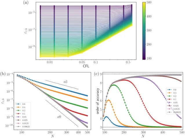
Several runs are carried out by varying the number of grid points (between100² and500²) and the CFL number (from 0.6 to 0.00625);

the errors measured after one cycle (i.e. when the vortex returns to the initial position for the first time) are shown inFig. 2, where each symbol denotes a run. It is worth pointing out that each simulation has been performed twice, with and without the shock-capturing term (𝑘₂=1and𝑘₂=0, respectively). As expected, differences were found to be negligible, with an influence on the 6th significant digit of the computed error norm. We then report hereafter only the results obtained for𝑘₂=1.Fig. 2a displays the value of the numerical error as a function of the CFL number for several grids (color plot). In order to recover the formal order of accuracy of the spatial discretization scheme for a given grid, the CFL number should be small enough not to affect𝜀_𝜏,ℎ; i.e.,𝜀_𝜏,ℎ should reach a plateau for sufficiently small values of the CFL number.

This is clearly visible inFig. 2a, which also highlights that even smaller CFL numbers should be considered for grids finer than500². InFig. 2b we report the error as a function of𝑁 for several CFL numbers. The order of accuracy of the numerical solution varies as expected between 3 to 9 (formal orders of the time integration and spatial discretization numerical schemes, respectively) as the CFL number gets smaller. For CFL numbers of 0.2 or smaller, a more or less extended region with ninth-order slope is observed; the slope tends to decrease for finer grids, due to the larger relative importance of the temporal error. The local slopes are shown inFig. 2c versus the number of grid points. The presence of a maximum can be explained by considering the temporal- to-spatial error ratio,𝛿. In order to keep a constant𝛿when refining the grid, the timestep should be decreased as𝜏∝ℎ^𝑞∕𝑝=ℎ^9∕3=ℎ³; whereas a constant CFL imposes𝜏∝ℎ(i.e., a varying𝛿). At CFL= 1.25 × 10⁻²

(7)

Fig. 1.Dispersion and dissipation errors as a function of the reduced wavenumber𝑘𝛿𝑥up to the ninth-order scheme. (a) dispersion error𝛷, (b) dissipation error𝐷.

Fig. 2. Analysis of the order of convergence of the error norm for the isentropic vortex convection configuration. (a): error of the𝐿₂-norm as a function of the CFL number for computational grids ranging from100² to500²; (b): error of the𝐿₂-norm as a function of the number of grid points for CFL numbers ranging from 0.6 to 0.00625; (c): overall spatio-temporal order of accuracy as a function of the number of grid points for CFL numbers ranging from 0.6 to 0.00625.

and6.25 × 10⁻³ the formal order of the spatial discretization scheme is recovered over the whole range of considered grid resolutions; this confirms previous studies suggesting the use of CFL≲0.01[71].

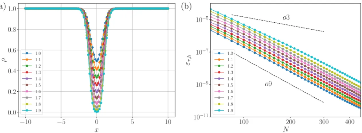
A parametric study on the influence of the maximum strength of the perturbation was also carried out. The value of𝛽in Eq.(37)was increased by a factor in the range [1, 1.9], with the minimum density value in the vortex core passing from𝜌_min≈ 0.5to𝜌_min≈ 4 × 10⁻³, as shown inFig. 3a. Fig. 3b shows that an increase of the perturbation strength leads to larger absolute values of the error norm, but does not alter substantially the formal order of accuracy of the numerical scheme.

4.2. Ideal-gas shock tube problems

The next test case is a classical benchmark for the assessment of shock-capturing capabilities. Specifically, we consider the well-known Sod [72] and Lax [73] 1D shock tube problems, corresponding to the following Riemann problems:

(𝜌, 𝑢, 𝑝)_SOD=

{(1,0,1) 𝑥 <0 (0.125,0,0.1) 𝑥≥0;

(𝜌, 𝑢, 𝑝)_LAX=

{(0.445,0.698,3.528) 𝑥 <0 (0.5,0,0.571) 𝑥≥0

(41)

(8)

Fig. 3. Analysis of the order of convergence of the error norm for the isentropic vortex convection configuration, for different values of the perturbation amplitude (from 1 to 1.9) at CFL= 0.025and𝑘₂= 1. (a): initial density profile at𝑦=0; (b): error of the𝐿₂-norm as a function of the number of grid points.

Fig. 4. Reference and numerical solutions for Sod’s (left) and Lax’s (right) shock tubes. Triangles: single species, circles: N₂-O₂mixture. The gray solid line denotes the reference solution.

Numerical results are compared to the exact solutions at the nondimensional time𝑡= 0.2(𝛥𝑡= 5 × 10⁻⁴) and𝑡= 0.13(𝛥𝑡=10⁻³), respectively.

For these test cases, the artificial viscosity coefficients are chosen equal to 𝑘₂ = 2, 𝑘₁₀ = 1∕630. The numerical domain is discretized with 200 evenly-spaced grid points; air is considered either as a single- species, calorically-perfect gas (𝛾= 1.4) or as a two-species non-reacting mixture of Nitrogen (𝑌_N

2 = 0.79) and Oxygen (𝑌_O

2 = 0.21). Fig. 4 shows the results for density, velocity and pressure, whose profiles are compared to the corresponding exact solutions. A good agreement is shown for both cases and the single-species and multi-species numerical solutions are perfectly superposed. The slight smearing of the numerical solution across the contact discontinuity can be attributed to the high- order dissipation term, the shock-capturing component being switched off in that region due to the constant value of the pressure. Note that a similar behavior is observed for other high-order schemes [18].

4.3. Shu-Osher problems

The Shu–Osher problem [74] consists of a𝑀=3shock propagating in a perturbed density field and allows to evaluate the behavior of the numerical scheme for a simplified shock-turbulence interaction configuration. The extent of the computational domain is[−5,5]and the initial conditions are

(𝜌, 𝑢, 𝑝)SHU=

{(3.857143,2.629369,10.33333) 𝑥 <−4

(1 + 0.2 sin(5𝑥),0,1) 𝑥≥−4 (42) The 1D Euler equations are solved on a uniform mesh with𝑁= 200and a reference solution is computed with the same numerical scheme on a

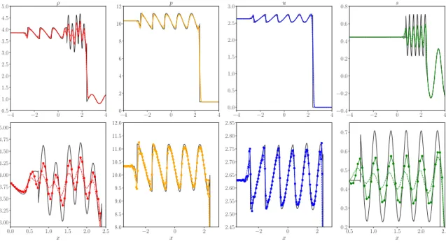
mesh with𝑁= 2000.Fig. 5shows results for density, pressure, velocity and entropy at the final time𝑡 = 1.8. The profiles of pressure and velocity are in good agreement with the reference solution, with some oscillations registered near the shock (which is captured reasonably well) that remain bounded to small values throughout the simulation.

On the contrary, the density and entropy profiles exhibit a stronger damping after the shock train passage. This is partly due to the use of a scalar artificial viscosity, which introduces the same amount of dissipation for all characteristic fields, whether they be of acoustic or entropic nature. Present results are in agreement with those of other classical numerical schemes [5]. Of note, the introduction of the Bhagatwala

& Lele correction to the shock-capturing term strongly enhances the entropy waves resolution (contrary to the shock tube cases, where no appreciable differences were found), mitigating the spurious activation of Jameson’s pressure-based sensor. A possible fix for this overly- dissipative behavior would be a selective reduction of the numerical dissipation by using different𝑘₂values for each equation. However, this approach would increase the number of tuning parameters, and was thus discarded in order to keep the numerical strategy as simple and general as possible. Lastly, it should be pointed out that the core regions of turbulent flows are intrinsically rotational: the Ducros sensor, which always degenerates to unity in 1D flows, plays therefore a fundamental role in minimizing the numerical dissipation outside of shocked-flow turbulent regions. For the purpose of comparison with other numerical strategies we also considered a two-dimensional generalization of the Shu–Osher problem, which consists in a vorticity/entropy wave interacting with a normal shock [5]. The extents of the computational domain are𝑥∈ [0,4𝜋), 𝑦∈ [−𝜋, 𝜋), with𝛥𝑥=𝜋∕50and𝛥𝑦= 𝜋∕16;

(9)

Fig. 5. Numerical solution for the Shu–Osher problem at𝑡= 1.8. Top: profiles of density, pressure, velocity and entropy; bottom: zoom on the post-shock regions. In each subfigure, the black solid lines denote the reference solution, and the colored solid and dashed lines the present solution, respectively with and without Bhagatwala & Lele’s correction.

periodic boundary conditions are imposed in the𝑦direction, whereas supersonic inflow and subsonic outflow are applied at𝑥= 0and𝑥= 4𝜋, respectively. The initial base flow reads

(𝜌, 𝑢, 𝑝)_SHU2D

=

{(𝜌_𝐿, 𝑢_𝐿, 𝑝_𝐿) = (1,1.5,0.714286) 𝑥 <3𝜋∕2 (𝜌_𝑅, 𝑢_𝑅, 𝑝_𝑅) = (1.862069,0.8055556,1.755952) 𝑥≥3𝜋∕2 (43) By superposing the combined vorticity/entropy wave, the initial data then becomes

⎧⎪

⎪⎨

⎪⎪

⎩

𝜌=𝜌+𝜌_𝐿𝐴_𝑒cos(𝑘_𝑥𝑥+𝑘_𝑦𝑦) 𝑢=𝑢+𝑢_𝐿𝐴_𝑣sin𝜓cos(𝑘_𝑥𝑥+𝑘_𝑦𝑦) 𝑣= −𝑢_𝐿𝐴_𝑣cos𝜓cos(𝑘_𝑥𝑥+𝑘_𝑦𝑦) 𝑝=𝑝

(44)

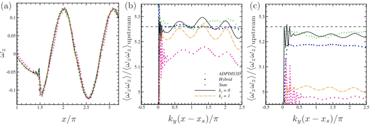
with𝐴_𝑒=𝐴_𝑣= 0.025,𝜓= 45^◦,𝑘_𝑥=𝑘_𝑦∕ tan𝜓and𝑘_𝑦equal to 1 or 2.

The vorticity content at𝑡= 25is reported inFig. 6and compared to results from the codes ADPDIS3D, Hybrid and Stan, digitalized from the Ref. [5] (the reader may refer to the original paper for details about the different shock-capturing approaches). Each test has been repeated twice, with 𝑘₂=0 and𝑘₂=1, to assess the influence of the shock-capturing term.

Both the instantaneous and mean quantities exhibit profiles of vorticity (Fig. 6) and kinetic energy (not shown) comparable to the reference. As expected, the shock-capturing activation reduces the post- shock oscillations and slightly damps the mean kinetic and vortical contents, which remain close to the reference linear analysis (LIA) results [75]. Interestingly, the post-shock mean vorticity profiles shows the same oscillating trend of the Stan code (which uses a LAD-based shock capturing), keeping however a better response in each case. We also note that for such a mild configuration, a lower value of𝑘₂would be more appropriate, resulting in a larger response.

4.4. Real-gas shock tube problem

The last inviscid test case consists of a multi-species, high- temperature shock tube designed by Grossman & Cinnella to study thermochemical effects [76]. For such a configuration, however, thermal nonequilibrium effects are rather mild and can be neglected, taking into

account only chemical nonequilibrium as shown in previous validation studies [71]. At𝑡= 0, the initial conditions are the following:

(𝑝, 𝑢, 𝑇)_GROSSMAN=

{1.95256 × 10⁵Pa, 𝑢_𝐿= 0 m∕s, 9000 K 𝑥 <0 10⁴Pa, 𝑢_𝑅= 0 m∕s, 300 K 𝑥≥0 (45) Chemically-reacting air is modeled by means of Park’s 5-species model (N₂, O₂, N, O, NO); the initial values for the species mass fractions cor- respond to the mixture equilibrium composition at the given pressure and temperature for the right and left states, respectively. Due to the stiffness of the chemical source terms, the solution is advanced in time using a CFL number of 0.02, as suggested in [76] for explicit Runge–

Kutta time integrations. The simulation is stopped when the shock-wave reaches the location𝑥= 0.11 m. Given the severe conditions developed by flow in the present problem, the Bhagatwala & Lele’s modification of the shock sensor was turned off for better numerical robustness.

Results at the final time are shown inFig. 7. The numerical scheme is able to capture correctly the rarefaction wave, the contact discontinuity and the shock; moreover, the distributions of the species mass fractions agree very well with data from [76].

5. Applications to multiscale turbulent flows

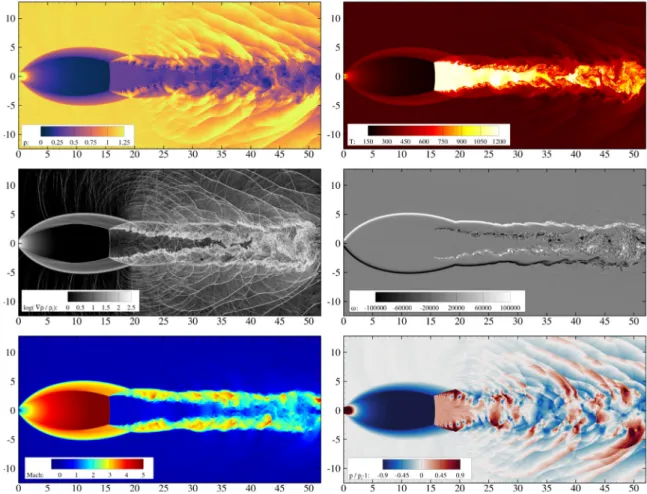
In this section we analyze the performance of the shock-capturing scheme for viscous compressible flows with shocks and fine-detail vortical structures. The applications range from a two-dimensional under-expanded jet flow to a hypersonic turbulent boundary layer in chemical nonequilibrium.

5.1. Two-dimensional underexpanded jet

A N₂-O₂inert, highly underexpanded jet has been first considered to test the suitability of the numerical scheme to deal with strong discontinuities and vortical layers in multi-species flows. This configuration represents the starting point for the study of reactive jets and has been widely analyzed in the past years, both experimentally and numerically.

In addition, it has been shown that 2D simulations are able to capture reasonably well some detailed features of the problem, such as the

(10)

Fig. 6. Results for the shock-vorticity/entropy wave interaction at𝑡= 25. (a) Instantaneous vorticity profiles for𝑦= 0(𝑘_𝑦= 1); averaged vorticity content, normalized with respect to the upstream value, for (b)𝑘_𝑦= 1and (c)𝑘_𝑦= 2. The shock location is𝑥_𝑠= 3𝜋∕2; the dashed horizontal lines in panels (b) and (c) denote the linear analysis solution [75].

Fig. 7. Profiles of density, pressure, velocity and mass fractions for the reacting, real gas shock tube case. In panels (a), (b) and (c), quantities are made non-dimensional with respect to the corresponding initial values on the right side of the tube. Lines: current simulation; symbols: reference solution [76].

location and dimension of the Riemann wave, the scale of the jet and the timewise averages of the thermodynamic variables.

The present setup is similar to the one reported in Martínez Ferrer et al. [77]. Specifically, the pressure 𝑃₀ and temperature 𝑇₀ of the mixture in the injection plane are set to 15 atm and 1000 K, whereas the ambient values are 1 atm and 300 K, respectively, resulting in a nozzle pressure ratio (NPR) of 15. The inflow jet Mach number is equal to 1 and a slow coflow at𝑀 = 0.05is imposed consistently with previous studies [77,78]. The height of the injector exit is equal to𝐷= 3 cmand the extent of the computational domain is𝐿_𝑥×𝐿_𝑦= 50𝐷× 25𝐷. At the inflow, the jet velocity is prescribed by means of an hyperbolic-tangent profile (see ‘‘Profile 2’’ of Michalke [79]):

𝑢(𝑟) 𝑈 =1

2 {

1 + tanh[ 0.25𝑅

𝜃 (𝑅

𝑟 − 𝑟 𝑅

)]}

(46)

where𝑈is the inflow centerline velocity,𝑅the inflow half-height,𝜃the initial momentum thickness of the shear layer and𝑟the local distance from the jet axis. The ratio𝑅∕𝜃is an important parameter influencing the jet stability, which is mainly related to the introduction of vorticity in the jet shear layer. In our study, we consider𝑅∕𝜃 = 12.5. At the remaining outflow boundaries, characteristic conditions are imposed, along with sponge regions and grid stretching to avoid spurious wave reflections.

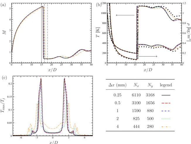
Five computational grids were considered, with dimensional mesh sizes equal to 𝛥𝑥 = 𝛥𝑦 = 4, 2, 1, 0.5 and 0.25mm. Fig. 8 shows an instantaneous snapshot of several quantities for the most refined grid used in the current study, revealing the challenging physics of the problem (for a thorough description of the flow physics of free underexpanded jets, the reader may refer to Franquet et al. [81]).