is an open access repository that collects the work of Arts et Métiers Institute of Technology researchers and makes it freely available over the web where possible.
This is an author-deposited version published in: https://sam.ensam.eu Handle ID: .http://hdl.handle.net/10985/8638
To cite this version :
Thomas LE GARREC, Xavier GLOERFELT, Christophe CORRE - Multi-Size-Mesh, Multi-Time- Step Algorithm for Noise Computation on Curvilinear Meshes - International Journal for Numerical Methods in Fluids - Vol. 74, n°1, p.1-33 - 2013
Any correspondence concerning this service should be sent to the repository Administrator : [email protected]
Computation on Curvilinear Meshes
T. Le Garrec1†, X. Gloerfelt1∗, C. Corre2
1DynFluid Laboratory - Arts et M´etiers ParisTech , 75013 Paris, France;2LEGI Laboratory - BP 53, 38041 Grenoble Cedex 9, France
SUMMARY
Aeroacoustic problems are often multiscale and a zonal refinement technique is thus desirable to reduce computational effort while preserving low dissipation and low dispersion errors from the numerical scheme.
For that purpose, the multi-size-mesh, multi-time-step algorithm of Tam and Kurbatskii [AIAA Journal, 2000,38(8), p. 1331-1339] allows changes by a factor of two between adjacent blocks, accompanied by a doubling in the time step. This local time stepping avoids wasting calculation time which would result from imposing a unique time step dictated by the smallest grid size for explicit time marching. In the present study, the multi-size-mesh, multi-time-step method is extended to general curvilinear grids by using a suitable coordinate transformation and by performing the necessary interpolations directly in the physical space thanks to multidimensional interpolations combining order constraints and optimization in the wavenumber space. A particular attention is paid to the properties of the Adams-Bashforth schemes used for time marching. The optimization of the coefficients by minimizing an error in the wavenumber space rather than statisfying a formal order is shown to be inefficient for Adams-Bashforth schemes. The accuracy of the extended multi-size-mesh, multi-time-step algorithm is first demonstrated for acoustic propagation on a sinusoidal grid and for a computation of laminar trailing edge noise. In the latter test-case, the mesh doubling is close to the airfoil and the vortical structures are crossing the doubling interface without affecting the quality of the radiated field. The applicability of the algorithm in 3D is eventually demonstrated by computing tonal noise from a moderate-Reynolds-number flow over an airfoil. Copyright c2012 John Wiley & Sons, Ltd.
Received . . .
KEY WORDS: computational aeroacoustics; zonal refinement; local timestepping; airfoil noise
1. INTRODUCTION
With the rapid advances in computational methodology, turbulence modeling and the availability of fast computers, noise investigations by Direct Noise Computation (DNC) [i.e. simulation of aerodynamic and acoustic quantities in the same run] are made possible. The main difficulty
∗Correspondence to: DynFluid Laboratory, Arts et M´etiers ParisTech, 151 boulevard de l’Hˆopital, 75013 Paris, France, E-mail: [email protected].
†Present address: ONERA, The French Aerospace Lab, 92322 Chatillon cedex, France.
of such simulations comes from the large disparities between the fine scales of turbulence and the large wavelengths of acoustic radiation which impose severe constraints on the meshes. In Computational Aeroacoustics (CAA), the preservation of the weak propagative waves with the turbulent motions can be achieved through the use of high-order finite differences in conjunction with structured meshes [1]. Local refinement is hardly achievable, and can lead to unacceptable grid sizes. The use of unstructured meshes, in conjunction with Discontinuous Galerkin method for instance [2], could be an alternative, but would still induce a significant computational cost.
Another attempt to preserve a high accuracy on structured or unstructured grids consists in the extension of the finite difference schemes in the finite volume context. Gaitonde and Shang [3]
propose the use of 4th-order compact finite volume schemes. An implicit deconvolution step relates cell averaged values to face values. The development of high-order compact deconvolution schemes is described by Kobayashi [4]. Pereira and Kobayashi [5] discussed the implementation for the incompressible Navier-Stokes equations. This strategy is pursued by Lacoret al. [6], who developed a multidimensional compact deconvolution for application to arbitrary meshes. In the compressible regime, Popescuet al. [7] propose to extend directly Dispersion-Relation-Preserving (DRP) or optimized prefactored scheme in the finite volume context. The high-order accuracy is obtained however at the price of an important extra cost. The Adaptative Mesh Refinement (AMR) method introduced by Berger and Oliger [8], or Roger and Colella [9] in the framework of Cartesian grids, allows local grid refinements but proves difficult to apply with high-order spatial schemes.
Moreover difficulties occur when the geometry is not Cartesian. Steinthorssonet al. [10] present an extension of the AMR technique for structured body fitted grids by using Hermite interpolations to generate the grid. The use of multi-grid or zonal grid technique is also commonly recognized as a useful method to increase the computational efficiency. The use of zonal grids has started with applications in meteorology, oceanography and atmospheric boundary layers and has then been used for turbulence simulations by DNS [11]; it has developed following two main strategies which are briefly reviewed to provide a non-exhaustive panorama of this rapidly expanding field.
In the first strategy, the grids can be generated independently for different zones or components and the grid overlap is allowed. Different zones or blocks get their boundary data using interpolation from neighboring blocks. Historically, the overset methods, also referred to as chimera methods, have been developed in the eighties by Benek et al. [12] or Steger et al. [13]. In the framework of CAA applications, Desquesnes et al. [14] proposed high-order overlapping grid method for coupling CFD and CAA; Sherer and Scott [15], Chicheportiche and Gloerfelt [16], or Daude et al. [17] considered many different interpolation techniques in order to determine the most accurate and robust ones for a wide range of applications.
In the second strategy, the mesh is generated by successive refinements at different grid levels, where the coarse grid solution is used as a boundary condition for the next finer grid level. The main drawback of this strategy is that without a coupling of the fine grid and coarse grid solutions, it will only provide coarse grid accuracy at the interfaces and will lead to some distorsions at the grid interfaces. Therefore, a special treatment has to be developed for the interface. In most of the cases, a high-order interpolation procedure for exchanging information between zones and a special treatment of the points near the interface are developed. Manhart [18] proposed a zonal method
with a second-order finite volume formulation. Kravchenko et al. [11] use spectral interpolations based on B-splines. In the present work, the multi-size-mesh multi-time-step strategy introduced by Tam and Kurbatskii [19, 20, 21] is followed: a doubling in the mesh size is accompanied by a doubling in the time step. The partitioning of the whole calculation domain allows local refinements and the number of grid points can thus be reduced. Tam and Kurbatskii [19] have considered Cartesian grids in their work. This method has been applied by Yin and Delfs [22] to rotor noise using a multi-domain Cartesian grid without the corresponding doubling of the time step. Tam and Ju [23] used both changes in the mesh size and time step in curvilinear meshes by working directly in the transformed elliptic coordinates. The use of a local time stepping alone has also been proposed. Allampalli and Hixon [24] used multi-time-step Adams-Bashforth schemes, in which different regions of the computational domain are made to march in time with different time steps. The multi-time-step strategy of Lin et al. [25] is designed for overset grids. No constraint is imposed on the ratio of mesh sizes between neighboring blocks thanks to a time interpolation used in the vicinity of the interface. L¨orcheret al. [26] propose to define a local time step for each cell of a Discontinous Galerkin method. The communication with neighbouring cells is ensured by solving a Cauchy-Kowalewski equation.
∆x ,
4 4∆t
x , 2∆t
∆ 2
∆x ,∆t
Figure 1. Changing in the mesh size and in the time step between three blocks.
In the present study, the multi-size-mesh, multi-time-step algorithm of Tam and Kurbatskii [20] is extended to general curvilinear grids by using a suitable coordinate transform and multidimensional interpolation directly in the curvilinear space. In the example of trailing edge noise from an airfoil, the local adaptation of the mesh size and of the time step can significantly reduce the computational effort. The numerical algorithm is presented in section 2, where discretization schemes on an 11-point stencils are derived for points near the doubling interface. The suitability of combining order constraints and optimization in the wavenumber space when deriving multidimensional interpolation coefficients is underlined. In section 3, a particular attention is devoted to the stability and accuracy properties of Adams-Bashforth schemes which are selected for time marching. Their efficiency is compared to Runge-Kutta methods. A first test-case for wave propagation is tackled in section 4 to check that the accuracy is preserved on sinusoidal grids. Laminar trailing edge noise from the flow over a NACA0012 airfoil at a Reynolds number based on the chord of Rec=5000 is used as a benchmark for the method in section 5. Finally, a three-dimensional example is given in
section 6 for the flow over a NACA0018 with an incidence of 6◦ and Rec=160 000, where tonal noise is expected.
2. NUMERICAL ALGORITHM 2.1. Governing equations
The compressible Navier-Stokes equations are solved in conservative form as
∂U
∂t + ∂
∂x(Fe−Fv) + ∂
∂y(Ge−Gv) = 0
whereU= (ρ, ρu, ρv, ρE)Tis the vector of unknowns. The inviscid (subscripte) and visco-thermal fluxes (subscriptv) are given by:
Fe= ρu, ρu2+p, ρuv,(ρE+p)uT
; Fv = (0, τxx, τxy, uτxx+vτxy−qx)T Ge= ρv, ρuv, ρv2+p,(ρE+p)vT
; Gv= (0, τxy, τyy, uτxy+vτyy−qy)T For an ideal gas, the specific total energyEis defined as
E=p/[(γ−1)ρ] + (u2+v2)/2, and p=ρrT,
whereT is the temperature,rthe gas constant, andγthe ratio of specific heats. The viscous stress tensorτijis modeled as a Newtonian fluidτij = 2µSij−(2/3)µSkkδij, whereSij = (ui,j+uj,i)/2 is the rate of strain tensor. Here µ is the dynamic molecular viscosity, approximated with Sutherland’s law:
µ(T) =µ0
T T0
32 T0+ 110.4 T+ 110.4
with T0=273.15 K and µ0=1.711×10⁵ kg.m−1.s−1. The heat flux componentqα models thermal conduction in theα-direction with Fourier’s lawqα=−(µcp/Pr)(∂T /∂xα), where Pr=0.72 is the Prandtl number, andcpis the specific heat at constant pressure.
The physical space (x,y) is mapped into a Cartesian regular computational space (ξ,η) thanks to coordinate transform. Consequently, large-stencil finite-difference schemes can easily be applied.
The geometrical mapping is characterized by its Jacobian matrix:
J =
∂ξ
∂x
∂η
∂x
∂ξ
∂y
∂η
∂y
=
ξx ηx
ξy ηy
(1)
The transformed equations can be written as follows [27,28]:
∂
∂t U
J
+ ∂
∂ξ 1
J(ξx(Fe−Fv)+ξy(Ge−Gv)
+ ∂
∂η 1
J (ηx(Fe−Fv) +ηy(Ge−Gv)
= 0
2.2. Specific centered finite-difference schemes
The 11-point centered optimized finite difference scheme of Bogey and Bailly [29] is used for approximating spatial derivatives at the interior points. The choice of an 11-point stencil scheme optimized in the wavenumber space has been proven to be a good trade-off in term of efficiency for wave propagation phenomena [29], and for large-eddy simulations of developed turbulence [30].
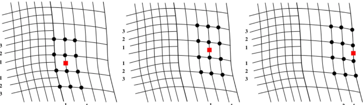
Furthermore, the explicit character of the scheme is well-suited to design special stencils for the mesh doubling. Indeed, when the grid size is double between two adjacent blocks as in Figure 1, five points of the fine block near the doubling interface require a particular treatment. The idea suggested by Tam and Kurbatskii [20,21] consists in building special stencils in order to keep centered schemes. The straightforward extension to an 11-point stencil is presented in Figure2. The five points located in the interface of the coarse block are easily dealt with by taking every two point of the fine block. Coefficients for 13- or 15-point stencils are given by Tam [21]. Note that other stencils could be considered, such as non-centered stencils [31], which introduce an additional dissipative error.
E D C B A
block 1 block 2
(a) (b)
A’
B’
C’
E’
D’
block 1 block 2
Figure 2. Buffer region between∆xand2∆xblocks, and specific centered stencils: (•) application point, (×) stencil. (a) The scheme is applied in the regular Cartesian computational space. (b) For the stencils at
points A’,B’,C’,D’,E’, the missing values represented by a red square () have to be interpolated.
At point B in Figure2(a), for instance, the first-order derivative(∂f /∂x)Bis approximated by:
∂f
∂x
B
= 1
∆x
5
X
j=1
aBj fjB−f−jB
(2)
where
f−jB =f(xB−∆B|j|x) j=-5,..,-1
fjB=f(xB+ ∆Bjx) j=1,..,5 (3)
∆B1x= ∆x, ∆B2x= 3∆x, ∆B3x= 5∆x, ∆B4x= 7∆x, ∆B5x= 9∆x (4) Following the DRP concept, the centered schemes are designed to minimize the dispersion error.
The effective wavenumberk⋆of the scheme is obtained by applying a spatial Fourier transform to Equation (2):
k⋆∆x=
5
X
j=1
aBj sin k∆Bj x
(5)
The coefficients aBj for an optimized scheme of order 4 on an 11-point stencil are calculated by satisfying the two first relationships canceling the terms of the Taylor expansions up to∆x4and by adding three relationships∂E/∂aBj = 0for1≤j≤3. The dispersion errorEis defined as [29]:
E=
Z ln(k∆x)h ln(k∆x)l
|k⋆∆x−k∆x|d(ln(k∆x))
whereln(k∆x)l=π/16andln(k∆x)h=π/2are chosen.
The same method is applied for points C, D and E with:
∆C1x= ∆x, ∆C2x= 2∆x, ∆C3x= 4∆x, ∆C4x= 6∆x, ∆C5x= 8∆x
∆D1x= ∆x, ∆D2x= 2∆x, ∆D3x= 3∆x, ∆D4x= 5∆x, ∆D5x= 7∆x
∆E1x= ∆x, ∆E2x= 2∆x, ∆E3x= 3∆x, ∆E4x= 4∆x, ∆E5x= 6∆x
For point A, the standard 11-point centered scheme [29] is used with a mesh size of2∆x. The calculated coefficient are given in TableI.
FD11A FD11B FD11C
a1 0.87502577558482 0.61534993594014 0.77608591242104 a2 -0.28944516727589 -0.05177798826851 -0.15880585249465 a3 0.09231030840505 0.01029785156943 0.01356408535315 a4 -0.02152267755252 -0.00190780289577 -0.00262508673197 a5 0.00260486879238 0.00020548792096 0.00037749644344
FD11D FD11E
a1 0.82482990265298 0.85768936001354 a2 -0.22249401437499 -0.26560173861406 a3 0.04320809837104 0.07376193338070 a4 -0.00210288198432 -0.01244166166264 a5 0.00014974870079 0.00033249395384
Table I. Coefficients of 11-point stencil finite-difference schemes of 4th-order and optimized in wavenumber space. FD11A means finite difference on eleven points at point A.
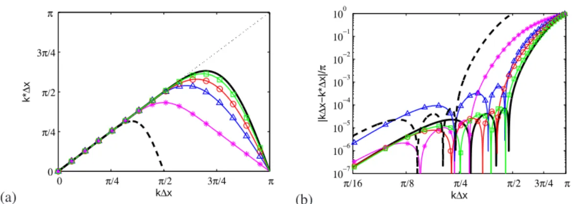
The dispersion error can be analysed in wavenumber space [32]. The effective wavenumbers resulting from the particular finite-difference schemes at points A, B, C, D and E, as defined by (5), are plotted in Figure3. The relationship for the scheme used at interior points with spacing∆xis also depicted. Note that at point A (Figure2), the stencil is that of interior points in the coarse grid with spacing2∆x. When plotted as a function ofk∆x, the Nyquist criterion yields a limit ofπ/2, explaining that the dashed line used for point A ends atπ/2. In Figure3(a), the deviation from the exact relationship, represented by the median line, indicates the limit of resolvability of the scheme.
First, it is worth noting that the curves for the stencils B to E lie in between those of interior points on the fine grid (solid line) and coarse grid (dashed line), respectively. A continuous transition from the coarse to the fine resolution (A to E) is important to reduce spurious reflection due to the grid- size mismatch. The dispersion error is plotted in Figure 3(b) on a logarithmic scale to highlight the limit of resolvability of each scheme. The resolvability is seen to be continuously reduced from
approximatelyπ/2(4∆xper wavelength) for the fine grid toπ/4(4×2∆xper wavelength) for the coarse grid.
(a)
0 π/4 π/2 3π/4 π
0 π/4 π/2 3π/4 π
k∆x
k*∆x
(b)
π/16 π/8 π/4 π/2 3π/4 π
10−7 10−6 10−5 10−4 10−3 10−2 10−1 100
k∆x
|k∆x−k*∆x|/π
Figure 3. (a) Effective wavenumberk∗∆xof the 11-point schemes as function of the reduced wavenumber k∆x: interior points on the fine grid ( ), E ( ), D ( ◦), C ( △), B ( ∗) and A (
) equivalent to interior points on the coarse grid. (b) Dispersion errors represented on a logarithmic scale.
2.3. Spatial filtering
Since a centered finite-difference scheme is systematically used, the differentiation is not dissipative. That is why a filtering procedure is employed to remove spurious high-frequency oscillations, which can be excited at the location of the interfaces and boundary conditions. An 11-point centered filter of tenth-order [33] is chosen for the two-dimensional laminar cases at moderate Mach numbers treated in the present study. Note that optimized filters would enhance the resolvability and would be beneficial for large-eddy simulations of turbulent flow, where the grid cut-off wavenumber is well inside the broadband energy spectrum [34].
New coefficients have been calculated for 11-point centered filters at the particular points A, B, C, D and E which use the same stencils as the corresponding finite difference schemes (Figure2).
For instance, at point B, a filtered variable is written as
ffiltered(xB) =f(xB)−χDf(xB) with 0≤χ≤1 and
Df(xB) =dB0f(xB) +
5
X
j=1
dBj(fjB+f−jB)
wherefjB andf−jB are defined by (3). The terms of the Taylor expansion are canceled up to∆x10 to obtain thedBj coefficients. In Fourier space, the relationshipDk(π) = 1is added, yielding the
following system:
dB0 + 2
5
X
j=1
dBj = 0
5
X
j=1
∆Bj x
∆x
!q
dBj = 0 1≤q≤4
dB0 + 2
5
X
j=1
(−1)
∆B jx
∆x
dBj = 1
where∆Bj is given by (4). The calculated coefficient are reported in TableII.
F11A F11B F11C F11D F11E
d0 63/256 1/2 11025/32768 9/32 525/2048
d1 -105/512 -19845/65536 -1/4 -3675/16384 -27/128
d2 15/128 2205/32768 735/8192 7/34 945/8192
d3 -45/1024 -567/32768 -147/16384 -441/16384 -5/128
d4 5/512 405/131072 9/8192 21/16384 27/4096
d5 -1/1024 -35/131072 -5/65536 -1/16384 -1/8192 Table II. Coefficients of tenth-order filters for the interface points.
The damping function is obtained by applying a spatial Fourier transform:
Dk(k∆x) =dB0 +
5
X
j=1
dBj cos(k∆Bj x) (6)
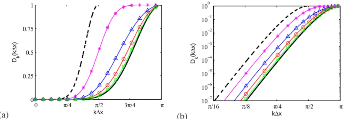
The transfer functions (6) of the filters at points A, B, C, D and E are compared in Figure4. The filter at point A is the standard tenth-order filter [33], used for interior points, with a double mesh size. The resolvability limit is progressively increased from point B up to point E. The smooth transition from scheme A to E ensures that disturbances at the block interfaces are minimized. In the following, the filtering procedure is applied every four timesteps withχ=0.2. It has been checked that changing the frequency of filtering or the amplitude coefficient does not change the results [35].
In fact, since the filter activity is restricted to high wavenumbers, well above the wavenumbers of interest, the results are weakly affected by the amplitude of the filtering.
2.4. Multi-dimensional interpolation scheme
The previous paragraphs have detailed the specific treatments developed to deal with the doubling of the mesh size along coincident mesh lines between the fine and coarse grids. Specific treatments must also be applied to deal with mesh lines from the fine grid with no counterpart in the coarse grid.
These treatments are described in the context of general curvilinear meshes. The values marked by squares in Figure2(b), located in the coarse grid, are used to differentiate the fluxes in the interface zone of the fine grid. These values are interpolated from known values at the nodes of the coarse grid, as depicted in Figure5.
For a Cartesian mesh, values can be interpolated with a directional interpolation technique. DRP optimized coefficients can be computed as proposed by Tam and Kurbatskii [36] for a 7-point
(a)
0 π/4 π/2 3π/4 π
0 0.25 0.5 0.75 1
k∆x Dk(k∆x)
(b)
π/16 π/8 π/4 π/2 π
10−7 10−6 10−5 10−4 10−3 10−2 10−1 100
k∆x D k(k∆x)
Figure 4. (a) Damping functions of the tenth-order filters at interior points on the fine grid ( ), particular point E ( ), D ( ◦), C ( △), B ( ∗) and A ( ) equivalent to interior points on the
coarse grid. (b) Damping functions on a logarithmic scale.
i−1 i i+1
j+3 j+2 j+1
j−1
j−3 j−2 j
j+3 j+2 j+1
j−1
j−3 j−2 j
i−1 i i+1
j+3 j+2 j+1
j−1
j−3 j−2 j
i i−1 i−2
Figure 5. Arrangement of the interpolation stencil (•) for different locations of the interpolated point () in the curvilinear physical space.
stencil, and extended by Gloerfelt [37] to 11-point stencil. When the mesh is no longer Cartesian, the data are exchanged in the curvilinear physical space and not in the Cartesian computational space. For that purpose a multi-dimensional interpolation scheme is proposed, taking into account the deformation of the interpolation stencil. For instance, the value at point(x0, y0)is interpolated from those of theNneighboring points(xk, yk):
u(x0, y0) =
N
X
k=1
Sku(xk, yk) (7)
The interpolation coefficientsSk are calculated by minimizing an error in the wavenumber space with constraints on the truncation order [38]. The method is detailed in chapter 13 of the textbook of Tam [21] in the context of overlapping grids. To preserve the high accuracy of the numerical algorithm, a 3×4 point stencil is chosen as depicted in Figure 5. The 12-point stencils allow the calculation of third-order interpolation coefficients optimized in the wavenumber space. The coefficients are computed and stored at the beginning of the simulation for each interpolation point.
(a)
O
x
x x
x x
x x
x
x x x
x
(b)
−1 −0.5 0 0.5 1
0 0.2 0.4 0.6 0.8 1
k1∆ k2∆
0.0001 0.0005
0.001 0.0025
0.005 0.01
0.015 0.02
0.0001 0.0005
(c)
−1 −0.5 0 0.5 1
0 0.2 0.4 0.6 0.8 1
k1∆ k2∆
0.0005 0.001
0.0025 0.005
0.01 0.015
0.0025 0.001 0.001
0.0001
(d)
−1 −0.5 0 0.5 1
0 0.2 0.4 0.6 0.8 1
k1∆ k2∆
0.0001 0.00050.001
0.0025 0.005
0.01 0.015
0.02
0.0001 0.0005
(e)
0 π/4 π/2 3π/4 π
0 0.2 0.4 0.6 0.8 1
k∆
|Elocal|
(f)
0 π/4 π/2 3π/4 π
10−7 10−6 10−5 10−4 10−3 10−2 10−1 100 101
k∆
|Elocal|
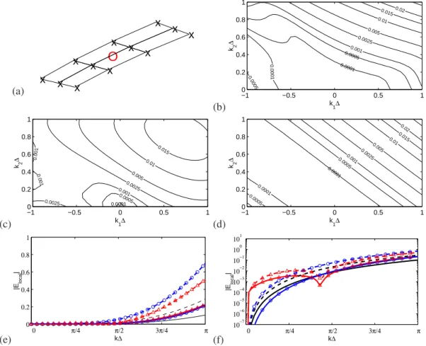
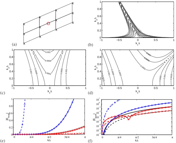
Figure 6. Multidimensional interpolation. (a) View of the interpolation stencil (×) and the interpolated point (◦). Maps of the local interpolation error (8) with coefficients calculated with: (b) order constraints alone;
(c) full optimization; (d) combination of order constraints and optimization procedure. Some profiles of the local interpolation error are proposed in (e) and (f) with linear and logarithmic scales, respectively: order constraints alone (b) alongy= 0( ◦) andx= 0( ◦); full optimization (c) alongy= 0(
△) andx= 0( △); combination of order constraints and optimization procedure (d) alongy= 0 ( ) andx= 0( ). The abscissa wavenumberkin plots (e) and (f) denotes eitherk1ork2for
horizontal and vertical profiles, respectively.
To better understand the interest of combining order constraints in the sense of Taylor expansions and minimization of an error in the wavenumber space, the local interpolation error, defined as
Elocal=
1−
N
X
k=1
Skeı(k1∆x(xk−x0)/∆x+k2∆y(yk−y0)/∆y)
(8) is plotted in Figures6and7for two representative shapes of the interpolation stencil. The particular stencil arrangements are shown in Figures 6(a) and7(a). Two-dimensional maps of the error in the reduced wavenumber space are represented by using the coefficients Sk resulting from the order constraints alone (Lagragian polynomials) in Figures6(b) and 7(b), Sk resulting from the full optimization in the wavenumber space in Figures6(c) and7(c) and finallySk resulting from the combination of order constraints and optimization in Figures6(d) and 7(d). The length scale
∆, used to form reduced quantities, corresponds to the mean of the|xi−xj|and|yi−yj|for the stencil. For the stencil of Figure6, the levels of error are greater for the fully optimized interpolation
shown in Figure6(c) than for the interpolation resulting from the sole order constraints in Figure 6(b). A quantitative comparison along the linesx= 0andy= 0is proposed in Figure6(e) and6(f) on a linear and logarithmic scale, respectively. On thex-axis, the optimization allows a reduction of the error for high wavenumbersk1∆> π/2, whereas the error (dashed line with△) is greater at low wavenumbers with respect to the interpolation with order constraints (◦), as observed on the logarithmic scale in Figure6(f). This increase of the error at low wavenumbers when the coefficients are deduced from optimization relationships is also visible along they-axis (solid lines with△ and
◦symbols). The optimized interpolation with added order constraints corresponds to the error map in Figure 6(d), which can be interpreted as a mix between Figures6(b) and 6(c). The associated error profiles in Figures6(e) and6(f) (solid lines without symbols) show that the new interpolation has the lowest errors at high wavenumbers (Fig.6(e)), whereas the low-wavenumber behavior is only slightly degraded with respect to the full order-constraint case. The combination of order constraints and optimization is thus an efficient way to enhance resolvability while preserving low levels of error at low wavenumbers. Its suitability is still more evident for the particular stencil of Figure7. The high levels of error in Figure7(b) when only order relationships are used is related to rank deficiencies of the corresponding system. The matrix is close to singular due to the almost alignments in they-direction. The error map in Figure7(c) for the full optimization is not sensitive to this kind of singularity. By combining order constraints and optimization in Figure7(d), the errors are substantially reduced in the x-direction. Adding order constraints is here again beneficial for improving low-wavenumber behavior of an optimized multidimensional interpolation. The better overall resolvability and isotropy of the error distribution are obtained by combining the order constraints and the optimization procedure for the determination of the interpolation coefficients.
3. TIME INTEGRATION SCHEMES
The previous section has described how non conformal mesh doubling are managed. The second essential ingredient of the algorithm is the local time stepping. The CFL condition of an explicit time advancement scheme sets indeed a unique time step dictated by the smallest cell dimension.
This leads to a waste of calculation time for every cell where the mesh size is significantly larger than this smallest scale. In the multi-size-mesh multi-time-step strategy, the time step is doubled if there is a corresponding doubling in the mesh size, as illustrated in Figure8. It can be noted in this figure that five points located in the interface zone belonging to the coarse grid need to be evaluated at intermediate time stepn+ 1/2to allow the evaluation of derivatives in the fine grid. Runge-Kutta schemes do not allow the marching of the interfaces at timen+ 1/2since they include fictitious intermediate stages to compute the numerical solution from timento timen+ 1. As suggested in the original method, Adams-Bashforth methods are selected to access the fluxes at intermediate timen+ 1/2, while preserving low dissipation and dispersion errors compatible with the chosen spatial discretization schemes.
(a)
O x
x x
x
x
x
x x x
x
x
x
(b)
−1 −0.5 0 0.5 1
0 0.2 0.4 0.6 0.8 1
k1∆ k2∆
0.0001 0.0050.03
(c)
−1 −0.5 0 0.5 1
0 0.2 0.4 0.6 0.8 1
k1∆ k2∆
0.0001 0.0005 0.001
0.0005 0.001
0.0005 0.001
(d)
−1 −0.5 0 0.5 1
0 0.2 0.4 0.6 0.8 1
k1∆
k2∆ 0.0001
0.0005 0.001
0.0005
0.001 0.0025
0.0001 0.0005 0.001 0.0025
(e)
0 π/4 π/2 3π/4 π
0 0.2 0.4 0.6 0.8 1
k∆
|Elocal|
(f)
0 π/4 π/2 3π/4 π
10−7 10−6 10−5 10−4 10−3 10−2 10−1 100 101
k∆
|Elocal|
Figure 7. Multidimensional interpolation. Same legend as Figure6for the particular stencil in (a).
n1 n2 n3
n3+1 n3+2
n1+1 n1+3 n1+4 n1+5 n1+6 n1+7 n1+8
n1+2
n2+4
n2+3
n2+2
n2+1
n2+1 2 n2+32 n2+5 2 n2+72
n3+21 n3+23
Block 3
Block 1 Block 2 mesh size
time step
Figure 8. Marching in time with a multi-time-step Adams-Bashforth method: five points, represented by red bullets, need to be advanced at intermediate time steps in the coarse grid interface zone.
3.1. Linear Multistep Methods
The high-order of accuracy is reached by using the informations from previous time steps. A Linear Multistep Method (LMM) with(p+ 1)levels is defined as
p
X
j=−1
ajUn−j+ ∆t
p
X
j=−1
bjf Un−j
= 0, (9)
whereaj andbj are coefficients,∆t is the advancement timestep, anda−1= 1is fixed. Explicit methods are obtained by choosingb−1= 0. For other values ofb−1, the algorithm is implicit. When aj = 0(j >0), only the fluxes at previous time steps are used. Adams-Moulton schemes constitute the implicit version, while explicit schemes are referred to as Adams-Bashforth methods.
3.1.1. Standard Adams-Bashforth schemes They are obtained by imposingaj = 0andb−1= 0in Equation (9). The equation∂U/∂t=F(U)can be integrated using the formula:
Un+1=Un+ ∆t
p
X
j=0
bj
∂U
∂t n−j
(10) where(p+ 1) denotes the number of time levels used in the integration formula. To ensure that the scheme remains consistent with the original equation, the coefficientsbj are chosen such that Equation (10) is satisfied to a prescribed order when both sides are expanded in Taylor series:
Un+1=Un+ ∆t∂Un
∂t +
∞
X
k=2
(∆t)k k!
∂kUn
∂tk
∂U
∂t
n−j
=∂Un
∂t +
∞
X
k=2
(−j∆t)k k!
∂k+1Un
∂tk+1
Identifying each term of the development leads to the following system of equations:
p
X
j=0
jmbj
m! = (−1)m 1
(m+ 1)! 0≤m≤p
3.1.2. Optimized Adams-Bashforth schemes Following Tam and Webb [39], the Laplace transform applied to (10) yields:
ω∗∆t= i(exp(−iω∆t)−1) Pp
j=0bjexp(ijω∆t) (11)
whereω∗is the effective angular frequency. The DRP procedure aims at minimizing the dissipation and the dispersion errors in the frequency space. The weighted integral errorEis written as
E=
Z ln(ω∆t)h ln(ω∆t)l
σ(Re(ω∗∆t−ω∆t))2+ (1−σ)(Im(ω∗∆t−ω∆t))2
d(ln(ω∆t)
where the upper and lower limits of the integral,(ω∆t)land(ω∆t)h, and the weightσhave to be chosen. Theσparameter between 0 and 1 allows to tune the optimization process so as to favor good wave propagation characteristics (real part of ω is emphasized) or good damping characteristics
(imaginary part ofω is emphasized). To derive an optimized scheme of orderq withp+ 1time- levels (q≤p+ 1), theqfirst relations obtained from Taylor series cancellation up to∆t(q−1)must first be satisfied, and(p+ 1−q)extra relations∂E/∂bj= 0(j=q−1top) are imposed, to yield p+ 1 equations with p+ 1 unknowns bj. Many coefficients for different number of time levels, scheme order and number of relations imposing ∂E/∂bj= 0 have been calculated. A 3rd-order, four-level scheme, with∂E/∂b3= 0, has been constructed as a compromise between the formal order, the number of optimized relations and the cost in memory storage induced by the number of levels.
This scheme is entirely defined once the following system is solved:
p
X
j=0
bj= 1 ;
p
X
j=0
jbj =−1 2!;
p
X
j=0
j2bj
2! = 1 3!;∂E
∂b3 = 0,
where(ω∆t)l= 0,(ω∆t)h=π/3andσ= 0.45. The computed coefficients are given in TableIII.
They are very close to those obtained by Tam and Webb [39], by optimizing with respect to the first coefficientb0with a slightly different definition of the error.
Coefficients Present Tam and Webb [39]
b0 2.24778466342984 2.30255809000000 b1 -2.32668732362284 -2.49100760333333 b2 1.41002065695617 1.57434093666667 b3 -0.33111799676317 -0.38589142333333
Table III. Coefficients of the3rd-order four-level Adams-Bashforth scheme optimized with respect tob3, and coefficients from Tam and Webb [39].
3.2. Comparison of the explicit time integration schemes
(a)
0 π/8 π/4 3π/8 π/2
0 0.5 1 1.5 2 2.5 3 3.5
ω∆t
|r|
(b)
0 π/3 2π/3 π 4π/3
0 0.5 1 1.5 2 2.5 3
ω∆t
|r|
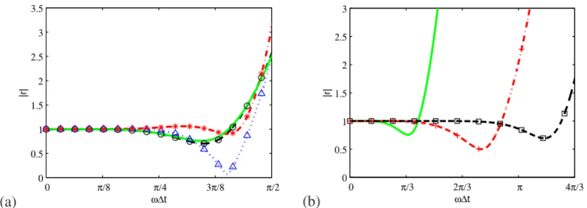
Figure 9. Growth factor r. (a) Comparison of different Adams-Bashforth schemes: standard 4th-order scheme ( ◦), standard5th-order scheme (· · · · △), standard6th-order scheme ( ∗) and 3rd-order optimized four-level scheme ( ). (b) Comparison of the 3rd-order optimized four-level scheme ( ) with the standard4th-order Runge-Kutta ( +) and low-storage2nd-order optimized
Runge-Kutta of Bogey & Bailly [29] with six sub-steps ( ).
3.2.1. Stability Stability investigations are realized by studying the growth factor, defined as g/ge=re−iϕ. For Adams-Bashforth schemes, we have:
g ge
= 1−iω∆t
p
X
j=0
bjexp (ijω∆t)
The modulerof the growth factor is plotted in Figure9(a) for different Adams-Bashforth schemes.
The numerical stability is preserved as long asr <1. This limit is slightly enlarged by choosing 5thor6th-order accuracy. This enlargement of the stability bound is, however, counterbalanced by a further restriction due to the spurious roots when a high order is considered, as will be observed thereafter. The comparison of3rd-order optimized and standard4th-order schemes using the same number of time levels indicates that the effect of the wavenumber optimization does not modify significantly the growth factor.
The limit of stability is compared with two Runge-Kutta schemes in Figure 9(b). An Adams- Bashforth scheme yields a lower stability bound. In practical terms, this means that the CFL number used with Adams-Bashforth schemes will be smaller than that of Runge-Kutta schemes. However, since Runge-Kutta schemes includepsub-steps while Adams-Bashforth schemes use a single step, the global calculation cost will remain roughly the same as demonstrated in§3.2.3.
4th-order AB
0 π/8 π/4 3π/8 π/2
−π/2
−π/4 0 π/4 π/2 3π/4 π
ω*∆ t
Re(ω∆ t)
5th-order AB
0 π/8 π/4 3π/8 π/2
−π/2
−π/4 0 π/4 π/2 3π/4 π
ω*∆ t
Re(ω∆ t)
3rd-order optimized AB
0 π/8 π/4 3π/8 π/2
−π/2
−π/4 0 π/4 π/2 3π/4 π
ω*∆ t
Re(ω∆ t)
0 π/8 π/4 3π/8 π/2
−π/2
−π/4 0 π/4 π/2
ω*∆ t
Im(ω∆ t)
0 π/8 π/4 3π/8 π/2
−π/2
−π/4 0 π/4 π/2
ω*∆ t
Im(ω∆ t)
0 π/8 π/4 3π/8 π/2
−π/2
−π/4 0 π/4 π/2
ω*∆ t
Im(ω∆ t)
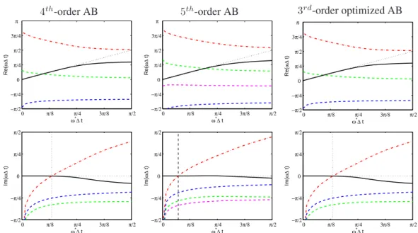
Figure 10. Real part (first row) and imaginary part (second row) of the roots ofω∆tas function ofω∗∆t. The solid line represents the physical root superimposed on the exact relationship (thin dotted line) at low frequencies. The dash-dotted line is the spurious root which yields the stability bound (marked by the vertical
dashed line in the plots of the imaginary part). The other spurious roots appear as dashed lines.
The analysis of the growth factorg/gecan be completed by the study of the roots of Equation (11). When multiplying this equation by the denominator of the right-hand side and byz=eiωt, we get a(p+ 1)th-order polynomial inz:
p
X
j=0
bjzj+1+ i
ω∗∆t(z−1) = 0
For instance a four-level scheme implies the existence of four roots ofω∆t as function ofω∗∆t, displayed in Figure 10. Among the roots, the physical one is such that its real part follows the exact relationship for frequencies lower thanπ/4. It is represented by the black solid line in Figure 10. The other roots correspond to spurious solutions of (11). The imaginary part of these roots is depicted on the second row of Figure 10. When the imaginary part is negative, a solution is damped in time, whereas a positive imaginary part lead to a solution growing in time and eventually to numerical instability. The effective stability bound thus corresponds to the reduced frequency where the spurious root represented with the red dash-dotted line crosses the positive axis. The same stability bound of 0.425 is noted for the two four-level schemes, namely AB4 of order 4 and ABo3 optimized of order 3. The scheme AB5 (5th-order Adams-Bashforth) is more unstable than AB4 with a stability bound of 0.225.
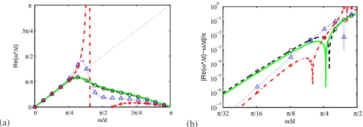
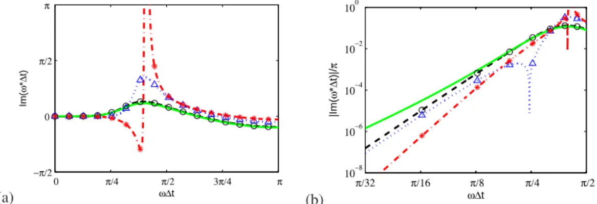
3.2.2. Dissipation and dispersion errors The real part of the effective angular frequency ω∗∆t is plotted in Figure 11 for the Adams-Bashforth schemes. The dispersion error, plotted on a logarithmic scale in Figure11(b), is smaller when the order of the standard schemes is increased.
However, for frequencies ω∆t > π/4, we can see in Figure 11(a) a large deviation from the exact relationship for the5th and6th-order schemes. The same large deviations nearπ/3are also noticeable for the imaginary part in Figure12(a) and can compromise the numerical stability. This tendency is intensified for the highest order since Adams-Bashforth schemes can be viewed as fully non-centered finite-difference schemes. Considering the low stability limit as determined by the previous analysis of spurious roots, only frequenciesω∆t.π/8are of interest in practice. In this frequency range, the dispersion and dissipation properties of the four-level optimized scheme are almost similar to the standard4th-order scheme. Since the DRP optimization is generally efficient to enhance the resolvality limit, this is useless when working only in the low-frequency range ω∆t.π/8. We can note in Figure 12(b) that the optimization procedure slightly increases the error of the imaginary part at low frequencies.
(a)
0 π/4 π/2 3π/4 π
0 π/4 π/2 3π/4 π
ω∆t
Re(ω*∆t)
(b)
π/32 π/16 π/8 π/4 π/2
10−7 10−6 10−5 10−4 10−3 10−2 10−1 100
ω∆t
|Re(ω*∆t)−ω∆t|/π
Figure 11. (a) Real part of the effective angular frequencyω∗∆tof Adams-Bashforth schemes as function of the exact angular frequency ω∆t: standard4th-order scheme ( ◦), standard5th-order scheme
(· · · · △), standard6th-order scheme ( ∗), and optimized3rd-order four-level scheme ( ).
(b) The errors are represented on a logarithmic scale.
3.2.3. Scalar advection of a wave packet A comparison between Runge-Kutta and Adams- Bashforth schemes is conducted to shed light on the dispersive and dissipative errors induced by
(a)
0 π/4 π/2 3π/4 π
−π/2 0 π/2 π
ω∆t
Im(ω*∆t)
(b)
π/32 π/16 π/8 π/4 π/2
10−8 10−6 10−4 10−2 100
ω∆t
|Im(ω*∆t)|/π
Figure 12. (a) Imaginary part of the effective angular frequency ω∗∆tof Adams-Bashforth schemes as function of the exact angular frequency ω∆t: standard4th-order scheme ( ◦), standard5th-order scheme (· · · · △), standard6th-order scheme ( ∗) and optimized3rd-order four-level scheme
( ). (b) The errors are represented on a logarithmic scale.
the time integration procedures. A simple linear scalar advection equationwt+awx= 0is used witha= 1. The test case consists in convecting a 1-D wave packet, defined at the initial time by
w(x) = sin 2πx
na∆x
exp −ln 2 x
nb∆x 2!
,
wherena∆xis the principal wavelength of the wave packet,nb∆xdenotes its Gaussian half width with ∆x= 1. The perturbation is convected over a distance of 800∆x by enforcing periodic conditions. Two initial configurations are tested here: one with 5 points per wavelength (na= 5, nb= 9) and the other with 6 points per wavelength (na= 6,nb= 9). The following integration methods are studied: the low-storage fourth-order Runge-Kutta scheme (RK4), the optimized six- sub-step Runge-Kutta (RK6) of Bogey and Bailly [29], the standard Adams-Bashforth schemes of order 3 (AB3), 4 (AB4) and 5 (AB5) and the third-order four-level optimized scheme (ABo3). The CFL number used for each scheme is given in TableIVand has been chosen to keep the overall cost identical. For example, the Adams-Bashforth schemes imply a single step, and their CFL number is thus divided by six compared with the six-sub-step Runge-Kutta algorithm. The 11-point-stencil DRP finite-difference scheme is used to compute the spatial derivativewx.
In order to compare the results, a mean quadratic error is computed as L=
sP
i(wi−wanal)2 P
iw2anal
The results for the different schemes and the different configurations are plotted in Figures 13 (na = 5,nb= 9) and14(na= 6,nb= 9). It can firstly be noted that the wave packets are hardly resolved by the third-order scheme. The standard RK4 scheme barely improves the results. On the other hand, AB4 and ABo3 schemes provide satisfactory results, which are almost similar, confirming the fact that the optimization has not a significant effect. The optimized scheme ABo3 even yields a quadratic error increased by 6% in the case (na= 6, nb= 9), compared with the standard AB4 with the same number of levels. No results for the AB5 scheme are given since this scheme is unstable. RK6 globally yields the better results. The errors Lare reported in TableIV.
3rd-order AB
−50 0 50
−1
−0.8
−0.6
−0.4
−0.2 0 0.2 0.4 0.6 0.8 1
x/∆ x
w
4th-order AB
−50 0 50
−1
−0.8
−0.6
−0.4
−0.2 0 0.2 0.4 0.6 0.8 1
x/∆ x
w
3rd-order optimized AB
−50 0 50
−1
−0.8
−0.6
−0.4
−0.2 0 0.2 0.4 0.6 0.8 1
x/∆ x
w
4th-order RK
−50 0 50
−1
−0.8
−0.6
−0.4
−0.2 0 0.2 0.4 0.6 0.8 1
x/∆ x
w
optimized RK6
−50 0 50
−1
−0.8
−0.6
−0.4
−0.2 0 0.2 0.4 0.6 0.8 1
x/∆ x
w
Figure 13. Advection of a wave packet withna= 5and nb= 9: numerical ( ) and analytical (◦ ◦ ◦) solutions.
The last line (na = 10,nb= 16) represents a packet discretized by a large number of points. In that case, AB4 can yield a lower error than RK6.
AB3 AB4 ABo3 RK4 RK6
CFL 1/6 1/6 1/6 2/3 1
(na= 5,nb= 9) 0.964 0.539 0.537 1.064 0.157 (na= 6,nb= 9) 0.809 0.284 0.302 0.985 0.174 (na= 10,nb= 16) 0.236 0.079 0.089 0.104 0.168
Table IV. Advection of a wave packet: mean quadratic errorsL, and values of the CFL number.
In summary, the DRP optimization applied to the Adams-Bashforth schemes does not improve significantly their overall resolvability compared to standard versions with the same number of levels. The standard fourth-order Adams-Bashforth has an efficiency comparable with an optimized Runge-Kutta scheme. That is why fourth-order Adams-Bashforth scheme is chosen in the present study.
3.3. Adams-Bashforth scheme at timen+ 1/2
To advance interfaces in time, the variables need to be calculated at time stepn+ 1/2since there is no information at this time for the points located on the coarse mesh side (see Figure8). An equation similar to (10) can be written at timen+ 1/2:
3rd-order AB
−50 0 50
−1
−0.8
−0.6
−0.4
−0.2 0 0.2 0.4 0.6 0.8 1
x/∆ x
w
4th-order AB
−50 0 50
−1
−0.8
−0.6
−0.4
−0.2 0 0.2 0.4 0.6 0.8 1
x/∆ x
w
3rd-order optimized AB
−50 0 50
−1
−0.8
−0.6
−0.4
−0.2 0 0.2 0.4 0.6 0.8 1
x/∆ x
w
4th-order RK
−50 0 50
−1
−0.8
−0.6
−0.4
−0.2 0 0.2 0.4 0.6 0.8 1
x/∆ x
w
optimized RK6
−50 0 50
−1
−0.8
−0.6
−0.4
−0.2 0 0.2 0.4 0.6 0.8 1
x/∆ x
w
Figure 14. Advection of a wave packet withna= 6and nb= 9: numerical ( ) and analytical (◦ ◦ ◦) solutions.
Un+12 =Un+ ∆t
p
X
j=0
b∗j ∂U
∂t n−j
(12) The conditions forpth-order accuracy are readily obtained:
p
X
j=0
jmb∗j
m! = (−1)m 1 (m+ 1)!
1 2
m+1
1≤m≤p
Coefficientsb∗j satisfying (12) up to∆t3 are given in TableVand compared with values provided by Tam and Kurbatskii [20], which are optimized in the wavenumber space with respect to the coefficientb∗0.
Coefficients Present Tam and Kurbatskii [20]
b∗0 295/384 0.773100253426 b∗1 −181/384 -0.485967426944 b∗2 101/384 0.277634093611 b∗3 −23/384 -0.064766920092
Table V.4th-order four-level Adams-Bashforth scheme at timen+ 1/2and coefficients of the 3rd-order optimized scheme of Tam and Kurbatskii [20].