Science Arts & Métiers (SAM)

Science Arts & Métiers (SAM)

is an open access repository that collects the work of Arts et Métiers Institute of Technology researchers and makes it freely available over the web where possible.

This is an author-deposited version published in: https://sam.ensam.eu Handle ID: .http://hdl.handle.net/10985/17473

To cite this version :

Mohamed JEBAHI, Lei CAI, Farid ABED-MERAIM - Strain gradient crystal plasticity model based on generalized non-quadratic defect energy and uncoupled dissipation - International Journal of Plasticity - Vol. 126, p.102617 - 2020

Any correspondence concerning this service should be sent to the repository Administrator : [email protected]

Strain gradient crystal plasticity model based on generalized non-quadratic defect energy and uncoupled dissipation

Mohamed JEBAHI^a,∗, Lei CAI^a, Farid ABED-MERAIM^a

aArts et Metiers Institute of Technology, CNRS, Université de Lorraine, LEM3, F-57000 Metz, France

Abstract

The present paper proposes a flexible Gurtin-type strain gradient crystal plasticity (SGCP) model based on generalized non-quadratic defect energy and uncoupled constitutive assumption for dissipative processes. A power-law defect energy, with adjustable order-controlling indexn, is proposed to provide a comprehensive investigation into the energetic length scale effects under proportional and non-proportional loading con- ditions. Results of this investigation reveal quite different effects of the energetic length scale, depending on the value of nand the type of loading. Forn ≥ 2, regardless of the loading type, the energetic length scale has only influence on the rate of the classical kinematic hardening, as reported in several SGCP works.

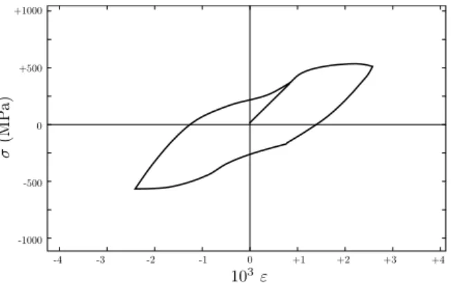
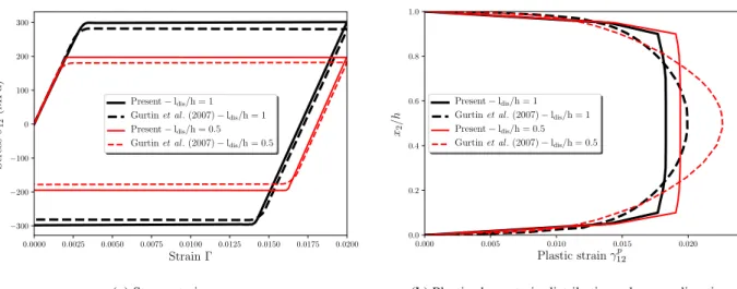
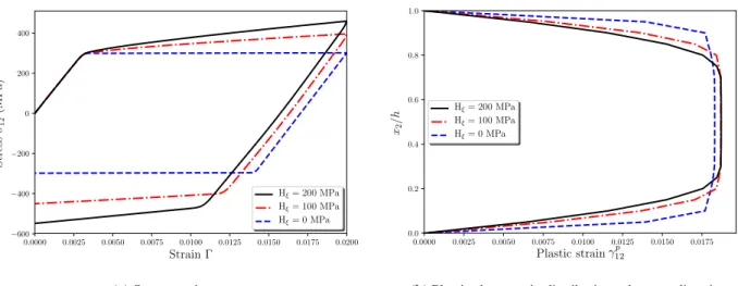
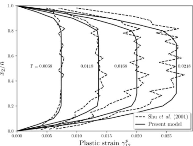
However, in the range of n < 2, this parameter leads to unusual nonlinear kinematic hardening effects with inflection points in the macroscopic mechanical response, resulting in an apparent increase of the yield strength under monotonic loading. More complex effects, with additional inflection points, are obtained un- der non-proportional loading conditions, revealing new loading history memory-like effects of the energetic length scale. Concerning dissipation, to make the dissipative effects more easily controllable, dissipative processes due to plastic strains and their gradients are assumed to be uncoupled. Separate formulations, expressed using different effective plastic strain measures, are proposed to describe such processes. Results obtained using these formulations show the great flexibility of the proposed model in controlling some major dissipative effects, such as elastic gaps. A simple way to remove these gaps under certain non-proportional loading conditions is provided. Application of the proposed uncoupled formulations to simulate the me- chanical response of a sheared strip has led to accurate prediction of the plastic strain distributions, which compare very favorably with those predicted using discrete dislocation mechanics.

Keywords: Strain gradient crystal plasticity, size effects, internal length scales, non-quadratic defect energy, uncoupled dissipation

1. Introduction

In the size range between hundreds of nanometers and few tens of micrometers, the strength of mate- rials is no longer scale-independent and the peculiar phenomenon “smaller is stronger” appears. This phe- nomenon has been revealed by several small scale experiments, such as micro-indentation (Ma et al.,2012;

Sarac et al.,2016;Dahlberg et al., 2017), micro-bending of thin foils (Hayashi et al., 2011) and torsion of thin wires (Liu et al.,2013). Conventional plasticity theories cannot predict the size-dependent behavior of materials, due to lacking internal length scale(s). To overcome this limitation,Aifantis(1984) has proposed in a pioneering work a strain gradient plasticity (SGP) model with a single internal length scale parameter embedded in the conventional plasticity theory. This model is capable of predicting plastic deformation

Email addresses:[email protected](Mohamed JEBAHI),[email protected](Lei CAI), [email protected](Farid ABED-MERAIM)

Preprint submitted to International Journal of Plasticity October 19, 2019

gradients (plastic inhomogeneities), which correlate with size effects as experimentally observed and nu- merically predicted using dislocation mechanics (Zhou and Lesar,2012;Dahlberg et al.,2017;Jiang et al., 2019). Plastic deformation gradients can physically be interpreted because they represent the geometrically necessary dislocations (GNDs; Ashby,1970), which are associated with small scale crystalline incompat- ibilities (e.g.,incompatibility of the mesoscopic plastic distortion). Interesting differential-geometry-based works studying, from a geometric point of view, the kinematics of these incompatibilities and their connec- tion with nonlocal (gradient) concepts can be found in the literature (Nye,1953;Bilby et al.,1955;Kröner, 1958;Kondo, 1964;Lardner,1969;Teodosiu and Sidoroff, 1976). Based on these works, Le and Stumpf (1996) andClayton et al.(2005) have proposed generalized theoretical frameworks capable of describing the finite deformation kinematics of several classes of crystalline defects in relation with gradient plasticity theories. Thanks to their capabilities in capturing size effects, the latter theories have received a strong sci- entific interest since the work ofAifantis(1984). This has led to the development of a wide variety of SGP models in the last two decades. According toHutchinson (2012), these models can be classified into two categories: (i) incremental models in which increments of higher-order stresses are related to increments of strain gradients, and (ii) non-incremental models in which the higher-order stresses themselves are expressed in terms of increments of strain gradients. Without claiming to be exhaustive, a brief review of such models is given hereafter. For more details about theoretical, numerical and experimental aspects of SGP theories, the reader is referred to the interesting review ofVoyiadjis and Song(2019).

The earliest SGP models proposed in the literature belong to the category of incremental models. In this context, Mühlhaus and Alfantis(1991) have elaborated a generalized version ofAifantis (1984) model by the inclusion of higher-order spatial gradients of the equivalent plastic strain in the yield condition. In a similar way,Acharya and Bassani(2000) have proposed a simple constitutive framework in which gradi- ent effects are incorporated in the hardening relations, using incompatibility-dependent hardening moduli.

These two models preserve the classical structure of the incremental boundary value problem (with con- ventional stresses, equilibrium equations and boundary conditions) and are referred to in the literature as lower-order SGP models. Fleck and Hutchinson (2001) have proposed a phenomenological higher-order SGP model with the purpose of generalizing the classical J2 flow theory to account for gradient effects at small scales. Both higher-order stresses and additional boundary conditions are considered and more than one material length scale parameters are covered in this model. However, the compatibility of such a model with the thermodynamic dissipation requirements (i.e., nonnegative dissipation) has not been addressed by the authors. Gudmundson (2004) has pointed out that the nonnegative dissipation cannot always be guar- anteed by this model. Later work of Gurtin and Anand (2009) has shown that this model is incompatible with thermodynamics unless the nonlocal terms are dropped. A modified version of this model in which the higher-order stresses are assumed to be fully energetic is proposed byHutchinson (2012) to ensure its thermodynamic consistency. The assumption of no higher-order contributions to dissipation has been used in subsequent works to develop thermodynamically-acceptable incremental models (e.g.,Fleck et al.,2015;

Nellemann et al.,2017,2018). However, the consistency of this assumption with the current understanding of dislocation physics is questioned. Until now, there are no acceptable recipes for an incremental model including higher-order dissipative stresses (Fleck et al.,2015).

To overcome the thermodynamic deficiency of the above class of models, while considering higher-order contributions to dissipation, several authors have proposed SGP models in which the higher-order stresses are expressed in terms of increments of plastic strain gradients. These models are classified as non-incremental in the classification ofHutchinson(2012). As examples of the pioneering models in this class, one can cite the models proposed byGurtin(2002,2004). The great success of such a class of models has made it the class the most studied in the literature in recent years. Consequently, a large number of interesting works associated with this class have recently been published. In a series of papers, Gurtin and coworkers (Gurtin et al., 2007;Gurtin,2008,2010;Anand et al.,2015) have developed several variations of single- and poly-crystal SGP models, in which GNDs are represented either by scalar dislocation densities or by the full dislocation

density tensor (Nye,1953). Mayeur and McDowell(2014) have shown that Gurtin-type models share several features with micropolar approaches (Mayeur et al.,2011). Polizzotto(2010,2014) has numerically studied different aspects of SGP theories in small and finite deformation frameworks. Yalçinkaya et al.(2011) and Klusemann and Yalçinkaya (2013) have proposed strain gradient crystal plasticity (SGCP) models with a non-convex part in the free energy to study the plastic deformation patterning (microstructure formation) and the localization phenomena in metals. For the same purposes, finite deformation SGP models have been proposed byAnand et al.(2012);Klusemann et al.(2013) andLing et al.(2018). In these models, the strain softening and localization are caused by the nonlinear geometric effects. Dahlberg and Faleskog(2014) have investigated the influence of the size and distribution of grains on the yield strength in poly-crystals using a SGP model and a grain boundary (GB) deformation mechanism. Wulfinghoff et al.(2015) have proposed a SGP model based on two formulations of defect energy to investigate their influence on the cyclic behavior of laminate microstructures. Bardella and Panteghini (2015) have applied a phenomenological distortion gradient plasticity model to study the effects of the plastic spin on the torsional response of thin metal wires. Bittencourt(2018) has focused on the numerical study of indentation problems using a SGCP model with two simplified hardening laws.Petryk and Stupkiewicz(2016) andStupkiewicz and Petryk(2016) have developed and studied a novel “minimal” framework of SGCP, including a variable internal length scale derived from physically-based dislocation theory of plasticity. The effects of this “natural” length scale on several existing SGCP models have been investigated by Ry´s and Petryk (2018). Based on these works, Dahlberg and Boåsen(2019) have proposed a new more general evolution equation for the length scale as a function of the plastic strains and their gradients. Compared to the class of incremental models, the present one always satisfies the thermodynamic requirements of nonnegative dissipation. However, as pointed out by several authors (e.g., Hutchinson, 2012;Fleck et al., 2014, 2015), it may lead in some cases to likely unacceptable results related to finite stress variation under infinitesimal loading change.

Despite the strong scientific effort on SGP theories, several related difficulties remain to be addressed.

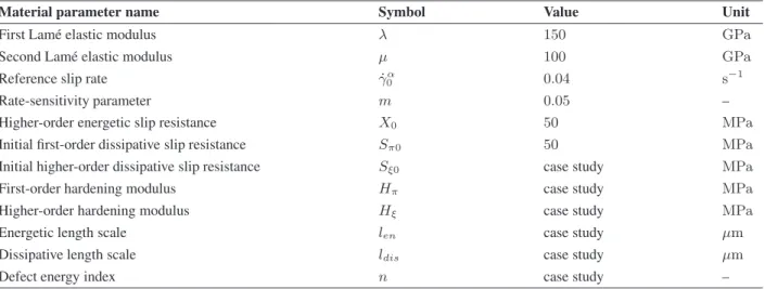
One of them is how to define the defect energy which conditions the higher-order energetic effects. In most existing SGP models, this energy is pragmatically assumed to be quadratic in plastic strain gradients (Gurtin, 2002,2004;Gurtin et al.,2007;Panteghini and Bardella,2016). Using this assumption,Gurtin et al.(2007) have shown that the energetic length scale effects have only influence on the rate of the classical kinematic hardening, but not on the material strengthening. Although this statement is widely recognized when using quadratic defect energy,Bardella and Panteghini(2015) have recently shown that accounting for plastic spin in this energy can lead to strengthening effects even if quadratic form is chosen. Despite their widespread use, quadratic forms are not usual in classical dislocation theories and several investigations have shown their inadequacy in the context of SGP (e.g., Cordero et al., 2010;Forest and Guéninchault, 2013). Mo- tivated by line tension arguments, rank-one (linear) defect energy has been used by several authors (e.g., Ohno and Okumura, 2007; Hurtado and Ortiz, 2013; Wulfinghoff et al., 2015). In most cases, this form shows strengthening effects of the energetic length scale. Bardella (2010) has studied the effects of the defect energy nonlinearity with quadratic and non-quadratic formulations involving plastic spin. Results by the author confirm the strengthening effects of the energetic length scale when using non-quadratic defect energy. Inspired by the statistical dislocation theory ofGroma et al.(2003),Forest and Guéninchault(2013) and Wulfinghoff et al.(2015) have proposed logarithmic form of defect energy. To overcome the problem of non-smoothness and non-convexity of this form, a quadratic regularization at small dislocation densities has been used (Wulfinghoff et al.,2015;Wulfinghoff and Böhlke,2015). El-Naaman et al. (2016) have in- vestigated two defect energy formulations with the aim of improving the micro-structural response predicted by SGP theories. A more complete investigation of these formulations using cyclic loading, as well as an interesting discussion about the origins of the strengthening effects of the energetic length scale, have very recently been published by the authors (El-Naaman et al.,2019). In almost all existing works on the subject, the higher-order energetic effects are studied using only proportional loading. The present paper aims to corroborate these works by proposing a comprehensive investigation of these effects under both proportional

and non-proportional loading conditions. To this end, a generalized power-law defect energy formulation, with adjustable order-controlling indexn, as a function of dislocation densities is proposed.

Another issue related to SGP theories is how to describe the dissipative processes. In almost all ex- isting strain gradient works, theses processes are considered to be coupled and described with the help of generalized effective plastic strain measures, which imply plastic strains and their gradients in a cou- pled manner (e.g.,Fleck and Hutchinson, 2001;Gurtin et al., 2007;Gurtin and Anand, 2009;Hutchinson, 2012;Fleck et al., 2015;Nellemann et al., 2017, 2018). This kind of (coupled) measures makes the issue of proposing robust and flexible dissipation formulations and the control of important dissipative effects difficult. Using coupled measures, it is not easy to control, for example, the elastic gaps at initial yield or at the occurrence of non-proportional loading sources. However, in most cases, the coupling between dissipative processes in the description of dissipation is only used by assumption. The existence of such a coupling in reality appears not to be physically confirmed. Based on the current understanding of dislo- cation physics, there exist no physical obstacles to assuming uncoupled dissipative processes. This can be confirmed by the contributions of Forest et al. (1997, 2000) and Forest and Sievert (2003). These authors have already adopted and extensively discussed uncoupling assumptions for the description of dissipative processes associated with force-stress and couple-stress quantities in the context of Cosserat plasticity the- ories. The resulting uncoupled-dissipation-based models are referred to in the literature as multi-surface or multi-criterion models. In the context of phenomenological strain gradient theories,Fleck et al.(2015) have also proposed uncoupled formulations for the description of dissipative processes associated with first- and higher-order stresses. In the same context, the very recent model proposed by Panteghini et al.(2019) can also be seen as a multi-criterion model. Indeed, several independent yield surfaces are introduced to describe the higher-order dissipation, which is considered to be independent of the first-order one. With the aim of ex- tending these works, and more particularly the work ofFleck et al.(2015), to strain gradient crystal plasticity, the present paper proposes a flexible uncoupled dissipation assumption to describe dissipative processes due to plastic slips and their gradients. These processes are assumed to be derived from a pseudo-potential that is expressed as a sum of two independent functions of plastic slips and plastic slip gradients. Conclusions about the physical consistency of this assumption will be drawn by comparing the associated results with others from the literature obtained using coupled dissipation.

Following this introduction, the present paper is organized as follows. Section2presents the proposed SGCP model, which is based on generalized non-quadratic defect energy and uncoupled dissipation. Section 3discusses the implementation of a simplified two-dimensional (2D) version of the proposed model. This version is used to investigate, in a simple manner, the effects of the model constitutive parameters on the global response of a crystalline strip subjected to proportional and non-proportional shear loading conditions.

Results of this investigation and discussions are presented in Section4. Section5presents some concluding remarks.

2. Strain gradient crystal plasticity (SGCP) model

In this section, a Gurtin-type strain gradient crystal plasticity (SGCP) model is developed based on gen- eralized non-quadratic defect energy and uncoupled dissipation, within the framework of small deformation.

2.1. Kinematics

Letu(x, t)denotes the displacement at timetof an arbitrary material point identified byxin a subregion V of the considered continuum. In the framework of small deformation, the displacement gradient∇ucan be additively split into elastic and plastic parts:

∇u=H_e+H_p (1)

whereH_eandH_prepresent respectively the elastic distortion, due to stretch and rotation of the underlying lattice, and the plastic distortion, due to plastic flow. Their symmetric parts define respectively the elastic and plastic strain tensors, and their skew-symmetric parts give respectively the elastic and plastic rotation tensors:

εe= 1 2

H_e+H^T_e

, εp = 1 2

H_p+H^T_p

, ωe= 1 2

H_e−H^T_e

, ωp = 1 2

H_p−H^T_p

(2) In single-crystal plasticity framework, it is widely acknowledged that plastic flow occurs through slip on prescribed slip systems, with each system αdefined by a slip directions^αand a slip-plane normalm^αunit vectors. With this description of plastic flow, the rate ofH_pcan be expressed as:

H˙_p = Xq α=1

˙

γ^α[s^αm^α] (3)

whereγ˙^α is the rate of plastic slip on slip systemα,q is the total number of slip systems, and “” is the tensor product operator. Using this expression, the plastic strain rate tensorε˙_pcan be written as:

˙ ε_p =

Xq α=1

˙

γ^αP^α (4)

whereP^αis the symmetrized Schmid tensor associated with slip systemα: P^α = 1

2(s^αm^α+m^αs^α) (5)

Equation (3), together with (1) and (2), can also be used to obtain a relation betweenu˙,ε˙e,ω˙eandγ˙^α:

∇u˙ = ˙εe+ ˙ωe+ Xq α=1

˙

γ^αs^α m^α (6)

In what follows,γandγ˙ (in bold) will be used to designate the list of plastic slips and their rates, respectively:

γ = γ¹, γ², ..., γ^q

, γ˙ = ˙γ¹,γ˙², ...,γ˙^q

(7) 2.2. Balance equations

The balance equations of the proposed strain gradient crystal plasticity (SGCP) model will be derived based on a generalization of the virtual power density of internal forces. In the present enhanced continuum, both displacement and plastic slip fields are considered as primary and controllable variables. As a conse- quence, the rates of these variables and their gradients will be involved in the definition of the virtual power density of internal forces:

{u˙,∇u˙,γ,˙ ∇γ}˙ (8)

The internal virtual power expended within a subregionV of the considered continuum is computed by means of densityp_intthat is assumed to depend linearly on all the virtual variations of the modeling variables given by (8):

p_int=f_i·δu˙ +σ :δ∇u˙ + Xq α=1

κ^αδγ˙^α+ Xq α=1

ξ^α·δ∇γ˙^α (9)

wheref_iis internal volumetric force,σis macroscopic stress tensor,κ^αandξ^αare respectively microscopic stress scalar (work-conjugate toγ^α) and microscopic stress vector (work-conjugate to∇γ^α) associated with slip system α, and “: ” is the double-dot product operator. The introduced microscopic stress scalar and vector are referred to hereafter as first- and higher-order microscopic stresses, respectively. Since the virtual power density of internal forces must be objective (i.e., independent of the frame in which the virtual varia- tions are expressed),f_imust be zero andσmust be symmetric. By using (6), it is then easy to demonstrate that:

p_int=σ:δε˙_e+ Xq α=1

(κ^α+τ^α) δγ˙^α+ Xq α=1

ξ^α·δ∇γ˙^α (10)

where τ^α is resolved shear stress on slip system α defined byτ^α = σ : (s^α m^α). Introducing a new first-order microscopic stress scalar π^α such that π^α = κ^α +τ^α, a more compact form of p_int, which is similar to that used byGurtin et al.(2007), can be obtained:

pint=σ:δε˙e+ Xq α=1

π^αδγ˙^α+ Xq α=1

ξ^α·δ∇γ˙^α (11)

Considering this expression of p_int, the internal virtual power expended within the subregion V can be expressed as follows:

P_int= Z

V

σ :δε˙_edv+ Xq α=1

Z

V

π^αδγ˙^αdv+ Xq α=1

Z

V

ξ^α·δ∇γ˙^αdv (12) Assuming that no external body forces act on the subregionVand the contact forces acting on its bound- aryS can be represented by a macroscopic traction vectort and a microscopic traction scalarχ^α on each slip systemα, the external virtual power expended onV can be expressed as:

Pext= Z

S

t·δu˙ds+ Xq α=1

Z

S

χ^αδγ˙^αds (13)

Application of the virtual power principle, which postulates that the internal and external virtual powers are balanced for any subregion V and virtual variations of the modeling variables, leads to two kinds of balance equations (since two kinds of primary variables are used). Macroscopic balance equations can be obtained by setting:

δγ˙ =0 (i.e., δ∇u˙ =δε˙_e+δω˙_e) (14)

Considering the symmetry of the stress tensor σ, after application of the Gauss (divergence) theorem, the virtual power balance becomes:

Z

V

(∇·σ)·δu˙ dv= Z

S

(σ·n−t)·δu˙ ds (15)

which is valid for any arbitrary subregion V and virtual variations of the modeling variables. This leads to the classical balance equations (static case) and the well-known traction conditions:

∇·σ = 0 in V

σ·n = t on S (16)

withnthe outward unit normal toS. The microscopic counterparts of these balance equations and boundary conditions can be obtained by setting:

δu˙ =0 (i.e., δε˙_e+δω˙_e =− Xq α=1

δγ˙^αs^α m^α) (17)

Considering (17), it can be demonstrated that:

σ :δε˙_e=− Xq α=1

τ^αδγ˙^α (18)

which leads, after application of the Gauss theorem, to the following form of the virtual power balance:

Xq α=1

Z

V

(τ^α+∇·ξ^α−π^α) δγ˙^αdv= Xq α=1

Z

S

(ξ^α·n−χ^α) δγ˙^αds= 0 (19) Since (19) is valid for any arbitrary subregionV and virtual variations of the modeling variables, the micro- scopic balance equation (static case) and the microscopic traction condition on each slip system αcan be obtained:

τ^α+∇·ξ^α−π^α = 0 in V

ξ^α·n = χ^α on S (20)

2.3. Dissipation inequality

The dissipation inequality in local form will be derived based on the second law of thermodynamics. In a mechanical perspective, this law can be expressed as follows: the temporal increase in free energy of any subregion V is less than or equal to the external power expended on this subregion. Mathematically, this means:

˙ Z

V

ψ dv≤ Pext (21)

where ψ is free energy per unit volume, which is assumed to be controlled by the following set of state variables: {ε_e,γ,∇γ}, as usually done in the framework of strain gradient crystal plasticity.

ψ=ψ(ε_e,γ,∇γ) (22)

Considering the identity P_int = P_ext , the above inequality can be rewritten in terms of internal power components as follows:

Z

V

ψ˙−σ : ˙ε_e− Xq α=1

π^αγ˙^α− Xq α=1

ξ^α·∇γ˙^α

!

dv ≤0 (23)

with

ψ˙(εe,γ,∇γ) = ∂ψ

∂ε_e : ˙ε_e+ Xq α=1

∂ψ

∂γ^α γ˙^α+ Xq α=1

∂ψ

∂∇γ^α ·∇γ˙^α (24)

SinceVis arbitrary, (23) yields the local dissipation inequality (also called local free energy imbalance):

D=σ : ˙εe+ Xq α=1

π^αγ˙^α+ Xq α=1

ξ^α·∇γ˙^α−ψ˙≥0 (25)

Replacingψ˙by its expression (24), this local inequality can be rewritten as follows:

D=

σ− ∂ψ

∂ε_e

: ˙ε_e+ Xq α=1

π^α− ∂ψ

∂γ^α

˙ γ^α+

Xq α=1

ξ^α− ∂ψ

∂∇γ^α

·∇γ˙^α≥0. (26) In the present SGCP model, the macroscopic stressσis regarded as energetic quantity having no contribution to dissipation:

σ = ∂ψ

∂ε_e (27)

whereas the microscopic stresses π^α and ξ^αon each slip system αmay possibly be divided into energetic and dissipative parts:

π^α =π_en^α +π^α_dis, ξ^α=ξ^α_en+ξ^α_dis (28)

with

π^α_en= ∂ψ

∂γ^α, ξ^α_en= ∂ψ

∂∇γ^α (29)

Therefore, the local dissipation inequality can be simplified as follows:

D= Xq α=1

π^α_disγ˙^α+ Xq α=1

ξ^α_dis·∇γ˙^α ≥0 (30)

This inequality will be considered in the definition of suitable constitutive laws for the dissipative micro- scopic stressesπ^α_disandξ^α_dison each slip systemα.

2.4. Constitutive laws

Constitutive relations are derived in this subsection to describe the evolution of the macroscopic and microscopic stresses involved in the balance equations (first lines of systems (16) and (20)), and then to reproduce the mechanical behavior of the considered continuum. This behavior is assumed to be governed by energetic and dissipative processes.

2.4.1. Energetic constitutive laws

The energetic processes are represented by the density of free energy ψ. In this work, the classical decomposition ofψinto an elastic strain energyψeand a defect energyψpis adopted. ψeis assumed to be a quadratic function ofε_e:

ψ_e(ε_e) = 1

2ε_e:C:ε_e (31)

where Cis the elasticity tensor, which is assumed to be symmetric and positive-definite. Building on the work ofGurtin et al.(2007),ψ_pis assumed to be function of dislocation densities:

ρ= ρ¹_⊢, ρ²_⊢, ..., ρ^q_⊢, ρ¹_⊙, ρ²_⊙, ..., ρ^q_⊙

(32) whereρ^α_⊢and ρ^α_⊙ denote respectively edge and screw dislocation densities on slip systemα. As shown by Arsenlis and Parks(1999), these quantities can be calculated by:

ρ^α_⊢=−s^α·∇γ^α, ρ^α_⊙=l^α·∇γ^α (33)

where l^α is the line direction of dislocation distribution defined by l^α = m^α×s^α (“×” is cross product operator). However, contrary to the work of Gurtin et al.(2007), in the present paper, ψ_p is assumed to be non-quadratic in these densities. A power-law form, with adjustable order-controlling indexn, is applied to define this energy:

ψ_p(ρ) = 1 nX0lⁿ_en

Xq α=1

|ρ^α_⊢|ⁿ+ ρ^α_⊙

ⁿ

(34) where X0 is a constant representing the energetic slip resistance, andl_enis an energetic length scale. To ensure the convexity ofψ_p, the defect energy indexnmust be greater than or equal to1(n≥1). Using (31) and (34), the free energy density can be expressed as:

ψ(εe,ρ) = 1

2ε_e :C:ε_e+ 1 nX0lⁿ_en

Xq α=1

|ρ^α_⊢|ⁿ+ ρ^α_⊙

ⁿ

(35) The partial derivatives of this expression with respect to the state variables presented in (22) provide the ener- getic constitutive laws that describe the evolution of the energetic stresses involved in the balance equations (first lines of systems (16) and (20)). The (energetic) macroscopic stress tensorσcan be expressed as:

σ = ∂ψ

∂ε_e =C:ε_e (36)

Since there is no explicit dependence between the assumed form of ψ and γ, the energetic part of the microscopic stress scalarπ_en^α is zero for any slip systemα:

π^α_en= ∂ψ

∂γ^α = 0 (37)

The energetic microscopic stress vectorξ^α_enon slip systemαcan be expressed as:

ξ^α_en= ∂ψ(ε_e,ρ)

∂∇γ^α =X0lⁿ_en h

|s^α·∇γ^α|ⁿ⁻² s^α⊗s^α+|l^α·∇γ^α|ⁿ⁻² l^α⊗l^αi

·∇γ^α (38) 2.4.2. Dissipative constitutive laws

As discussed in the introduction, in almost all existing strain gradient theories involving both first- and higher-order dissipative microscopic stresses, the evolution of the latter is described using constitutive equa- tions based on generalized effective plastic strain measures, which imply plastic strains and their gradi- ents in a coupled manner (e.g.,Fleck and Hutchinson, 2001; Gurtin et al., 2007; Gurtin and Anand,2009;

Hutchinson,2012;Fleck et al.,2015;Nellemann et al.,2017,2018). An example of these measures is:

E˙_p = q

kε˙_pk²+l²_dis k∇ε˙_pk², E_p =

Z E˙_pdt (39)

wherel_disis a dissipative length scale. However, the use of such coupled measures to define the dissipative constitutive equations largely restricts their flexibility and makes the control of some numerically noticed unusual behaviors,e.g., the elastic gap at initial yield (Hutchinson,2012;Fleck et al.,2015), difficult. Actu- ally, in most cases, these coupled measures are only used by assumption, as the coupling between first- and higher-order dissipative processes is hitherto not physically confirmed.

To allow for more flexible control of major dissipative effects, in present work, the dissipative micro- scopic stresses are derived from a dissipation functional ϕ, which is postulated based on the assumption of uncoupled dissipative contributions from plastic slips and plastic slip gradients. In spirit of multi-criterion approaches available in the literature (Forest et al.,1997,2000;Forest and Sievert,2003;Fleck et al.,2015;

Panteghini et al.,2019), this functional is assumed to be divided into two independent parts: one part, which describes first-order dissipative effects, is only function of plastic slips and their ratesϕ_π; and the other part, which describes higher-order dissipative effects, depends only on gradients of plastic slips and their rates ϕ_ξ. Note that similar (uncoupling) assumption was applied in the recent contribution ofFleck et al.(2015) to describe first- and higher-order dissipative effects in the context of phenomenological strain gradient plas- ticity. Therefore, the present work can be seen as an extension of this contribution to strain gradient crystal plasticity.

Define independent first- and higher-order effective plastic strains for each slip system α (e^α_π and e^α_ξ, respectively) as follows:

˙

e^α_π =|γ˙^α|= q

( ˙γ^α)², e^α_π = Z

˙

e^α_πdt (40)

˙

e^α_ξ =kl_dis∇^αγ˙^αk=l_dis q

(∇^αγ˙^α)², e^α_ξ = Z

˙

e^α_ξ dt (41)

where∇^αis the projection of∇onto slip systemα:

∇^αφ= (s^α·∇φ) s^α+ (l^α·∇φ) l^α (42) The proposed uncoupled dissipation functional can be expressed as:

ϕ( ˙e_π,e_π,e˙_ξ,e_ξ) = ϕπ( ˙e_π,e_π) +ϕ_ξ( ˙e_ξ,e_ξ) (43) with

˙

e_π = ˙e¹_π,e˙²_π, ...,e˙^q_π

, e_π = e¹_π, e²_π, ..., e^q_π

, e˙_ξ =

˙

e¹_ξ,e˙²_ξ, ...,e˙^q_ξ

, e_ξ=

e¹_ξ, e²_ξ, ..., e^q_ξ

(44) For comparison purposes, expressions of ϕ_π and ϕ_ξ are postulated in such a way as to obtain dissipative microscopic stresses having forms close to those proposed byGurtin et al.(2007):

ϕ_i( ˙e_i,e_i) = Xq α=1

S_i^α γ˙₀^α m+ 1

e˙^α_i

˙ γ₀^α

m+1

(45) where the subscript i takes as value π or ξ in reference to first- or higher-order dissipative microscopic stresses, γ˙₀^α > 0 is a constant strain rate representative of the flow rates of interest, m > 0is a constant characterizing the rate-sensitivity of the considered material, and S_i^α (i ∈ {π, ξ}) are stress-dimensional internal state variables (S^α_π > 0and S_ξ^α ≥ 0). These variables are referred to hereafter as dissipative slip resistances and their evolutions are assumed to be governed by:

S˙_i^α = Xq β=1

h^αβ_i S_i^β

˙

e^β_i with S_i^α(0) =S_i0 (46)

S_i0(i∈ {π, ξ}) are initial dissipative slip resistances (withS_π0 >0andS_ξ0 ≥0), andh^αβ_i (i∈ {π, ξ}) are positive hardening moduli assumed to evolve according to:

h^αβ_i S_i^β

= s^αβh_i S_i^β

| {z }

+ l^αβh_i S_i^β

| {z } Self hardening Latent hardening

(47)

s^αβ is self hardening parameter marking coplanar slip planes and is defined by:

s^αβ =

1 if m^α∧m^β =0

0 otherwise (48)

andl^αβ is latent hardening parameter defined in this work as:

l^αβ = s^α·s^β

m^α∧m^β

(49)

to take into account the influence of the relative misorientation of slip planes on the hardening moduli.

hi (i ∈ {π, ξ}) are self-hardening functions which, motivated by several works from the literature (e.g., Kalidindi et al.,1992;Gurtin et al.,2007), are assumed to be defined as:

h_i S_i^β

=





 H_i

1− ^S

β i

SiF

a

for S_i0≤S_i^β < S_iF

0 for S_i^β ≥SiF

(50) withS_iF > S_i0,a≥1andH_i ≥0.

Based on the above definitions of the ingredients of the proposed dissipation functionalϕ, it can easily be verified that this functional is nonnegative and convex inγ˙^αand∇γ˙^α, which guarantees a priori satisfaction of the second principle of thermodynamics (nonnegative dissipation). The partial derivatives of ϕ with respect to γ˙^α and ∇γ˙^α give the expressions of the dissipative stress scalar π^α_dis and vector ξ^α_dis on slip systemα:

π_dis^α = ∂ϕ

∂γ˙^α =S_π^α e˙^α_π

˙ γ₀^α

m

˙ γ^α

˙

e^α_π (51)

ξ^α_dis = ∂ϕ

∂∇γ˙^α =S_ξ^αl_dis² e˙^α_ξ

˙ γ₀^α

m

∇^αγ˙^α

˙

e^α_ξ (52)

As mentioned above, the dissipation functional proposed in this work ϕ leads to dissipative microscopic stresses close to those postulated by Gurtin et al. (2007) based on the normality rule. The latter can be obtained from (51) and (52) by replacing the first- and higher-order effective plastic strains by a coupled one defined by:

d˙^α= r

( ˙e^α_π)²+

˙ e^α_ξ2

, d^α = Z

d˙^αdt (53)

and by replacingS^α_π andS_ξ^αby a single strictly positive slip resistanceS^αcalculated based ond˙^α.

2.5. Flow rules

Based on the expressions of the microscopic stresses, the microscopic balance equation associated with slip systemα(first line of system (20)) can be reformulated as follows:

τ^α+∇·ξ^α_en+∇·ξ^α_dis−π^α_dis= 0 (54)

When augmented by the microscopic constitutive laws (38), (51) and (52), this equation acts as a flow rule associated with slip systemα:

τ^α+∇·ξ^α_en+∇· (

S^α_ξ l²_dis e˙^α_ξ

˙ γ₀^α

m

∇^αγ˙^α

˙ e^α_ξ

)

−S_π^α e˙^α_π

˙ γ₀^α

m

˙ γ^α

˙

e^α_π = 0 (55)

Bearing in mind (38),∇·ξ^α_encan be expressed as:

∇·ξ^α_en = A^αα :∇∇γ^α (56) with

A^αα = (n−1) X0lⁿ_en h

|s^α·∇γ^α|ⁿ⁻² s^α⊗s^α+|l^α·∇γ^α|ⁿ⁻² l^α⊗l^αi

(57) Using (56), the flow rule (55) becomes:

τ^α+A^αα :∇∇γ^α+∇· (

S_ξ^αl²_dis e˙^α_ξ

˙ γ₀^α

m

∇^αγ˙^α

˙ e^α_ξ

)

−S_π^α e˙^α_π

˙ γ₀^α

m

˙ γ^α

˙

e^α_π = 0. (58)

The second term in the above equation, being energetic, represents the negative of a backstress, leading to Bauschinger effects in the flow rule. The last two terms of this equation are dissipative (resulting from the dissipation functional). A reversal of the flow direction (γ˙^α → −γ˙^α) simply changes their sign. Therefore, these terms represent the dissipative (isotropic) hardening. The flow rule (58) can then be written in a more convenient form as:

τ^α − (−A^αα :∇∇γ^α)

| {z }

= S_π^α e˙^α_π

˙ γ₀^α

m

˙ γ^α

˙

e^α_π −∇· (

S_ξ^αl²_dis e˙^α_ξ

˙ γ₀^α

m

∇^αγ˙^α

˙ e^α_ξ

)

| {z }

Energetic backstress Dissipative hardening

(59)

3. Simplified two-dimensional version of the SGCP model and numerical implementation

In this section, a simplified two-dimensional (2D) version of the proposed SGCP model is derived and implemented to investigate, in a simple manner, the influence of the constitutive parameters and the uncou- pled dissipation functional on the global response of the considered continuum.

3.1. Simplified 2D SGCP model

The plane strain condition is adopted for the 2D model. Under this condition, the displacement field can be degenerated as:

u(x, t) =u1(x1, x2, t) e1+u2(x1, x2, t) e2 (60) which results in a displacement gradient ∇uthat is independent ofx3. Furthermore, attention is restricted to planar slip systems,i.e., slip systems satisfying:

s^α·e₃ = 0, m^α·e₃= 0, s^α×m^α=e₃ (61)

with slipsγ^αindependent ofx3. All other slip systems are ignored. This approximate assumption is widely used in the literature under plane strain, as it allows for constructing simple 2D constitutive models. Using this assumption, it can be shown that:

e₃·∇γ^α= 0 and l^α=m^α×s^α=−e₃ (62) which implies that screw dislocations vanish:

ρ^α_⊙=l^α·∇γ^α = 0, ∀α∈ {1, 2, ..., q} (63) Ignoring the crystalline elastic anisotropy and using the proposed form of defect energy (34), with only edge dislocation densities, the energetic macroscopic and microscopic stresses involved in the simplified model can be expressed as:

σ = λtr (εe) I+ 2µεe

π_en^α = 0 ξ^α_en = X0l_enⁿ h

|s^α·∇γ^α|ⁿ⁻² s^α⊗s^αi

·∇γ^α

(64)

whereλandµare the first and second Lamé elastic moduli. Concerning the dissipative microscopic stresses, simplified equations obtained from (51) and (52), with the slip resistances S_π^α and S_ξ^α assumed to evolve linearly with the effective plastic strains, are used to define these stresses:

π_dis^α = S_π^α e˙^α_π

˙ γ₀^α

m

˙ γ^α

˙ e^α_π ξ^α_dis = S_ξ^αl²_dis

e˙^α_ξ

˙ γ₀^α

m

∇^αγ˙^α

˙ e^α_ξ

(65)

where, fori∈ {π, ξ}:

S˙_i^α = Xq β=1

H_ie˙^β_i with S^α_i (0) =S_i0, H_i = constant≥0 (66) Note thatS_π0>0andS_ξ0≥0.

In summary, the overall constitutive equations of the simplified 2D SGCP model are:











































σ =λtr (εe) I+ 2µεe

ξ^α =X0lⁿ_en h

|s^α·∇γ^α|ⁿ⁻² s^α⊗s^αi

·∇γ^α+S_ξ^αl_dis² e˙^α_ξ

˙ γ₀^α

m

∇^αγ˙^α

˙ e^α_ξ π^α =S_π^α

e˙^α_π

˙ γ₀^α

m

˙ γ^α

˙ e^α_π S˙_π^α =

Xq β=1

H_πe˙^β_π , S_π^α(0) =S_π0>0 S˙_ξ^α =

Xq β=1

H_ξe˙^β_ξ , S_ξ^α(0) =S_ξ0 ≥0

˙

e^α_π =|γ˙^α|, e˙^α_ξ =kldis∇^αγ˙^αk α= 1,2, ..., q

(67)

These equations are solved numerically within the framework of finite element method. A brief presentation of the numerical procedure is presented in the next subsection.

3.2. Numerical implementation

The weak forms of the macroscopic and microscopic balance equations (first lines of systems (16) and (20)) may be formulated using the virtual power relations given in section2. Here, the virtual fieldsδu˙ and δγ, which are referred to as test fields, are assumed to be kinematically admissible to˙ 0 on the portions of the boundary of the studied domain on which Dirichlet (essential) boundary conditions are imposed. The macroscopic and microscopic weak forms can then be respectively expressed as:

G_u = Z

V

δε˙ :σdv− Z

St

δu˙ ·tds G_γ =

Xq α=1

Z

V

∇δγ˙^α·ξ^αdv+ Xq α=1

Z

V

δγ˙^απ^αdv− Xq α=1

Z

V

δγ˙^αP^α:σdv− Xq α=1

Z

S^α_χ

δγ˙^αχ^αds (68)

where S_t and S_χ^α are respectively the portions of the domain boundary on which macroscopic and micro- scopic traction forces, respectively noted astandχ^α, are imposed.

To numerically solve these weak forms, a User-ELement (UEL) subroutine is implemented within the commercial finite element package ABAQUS/Standard. Both displacement and plastic slip fields (u and γ) are considered as degrees of freedom in the UEL. Isoparametric two-dimensional eight-node quadratic elements are used. Integration within these elements is carried out using 9-point Gaussian technique. In each element, displacement fieldsui(i∈ {1,2}) and plastic slip fieldsγ^α(α∈ {1,2, ..., q}) are approximated based on nodal values as follows:

u_i(x1, x2) = X8 k=1

N_k(x1, x2)U_i^k, γ^α(x1, x2) = X8 k=1

N_k(x1, x2) Γ^α_k (69) whereU_i^k andΓ^α_k are respectively the nodal values of displacement u_i and plastic slipγ^α, andN_k are the interpolation (shape) functions, which are assumed to be the same for both displacement and plastic slip fields. Using these field approximations, the above weak forms can be written, in matrix form, within a representative finite element as:

G^e_u = δU˙^eT

· Z

V^e

B^T

u ·σ dv− Z

S_t^e

N^T

u ·t ds

!

G^e_γ = δ˙Γ^eT

· Z

V^e

B^T

γ ·ξ dv+ Z

V^e

N^T

γ ·π dv− Z

V^e

N^T

γ ·τ dv− Z

S_χ^e

N^T

γ ·χ ds

! (70)

whereσ,πandξare vector representations of the macroscopic stress and the microscopic stresses on all slip systems,τ is a vector containing the resolved shear stresses on all slip systems,tis the macroscopic traction vector,χis a vector containing the microscopic tractions on all slip systems, N

u andB

u are interpolation and gradient matrices associated with the displacement field, andN_γandB_γare interpolation and gradient matrices associated with the plastic slip fields. Expressions of these vector and matrix quantities are long and not revealing, they are not presented in this paper.

The principle of virtual power implies thatG^e_u andG^e_γare zero for any virtual variations of the element nodal variablesδU˙^eandδ˙Γ^e. Therefore:

R^e_u = Z

V^e

B^T

u ·σ dv− Z

S_t^e

N^T

u ·t ds = 0

R^e_γ = Z

V^e

B^T_γ ·ξ dv+ Z

V^e

N^T_γ ·π dv− Z

V^e

N^T_γ ·τ dv− Z

S^e_χ

N^T_γ ·χ ds = 0

(71)

These equations are linearized with respect to the variations of the element nodal variablesU^eandΓ^e, which results in an elementary system of linear equations that can be presented in matrix form as follows:

"

K^e_uu K^e_uγ K^e_γu K^e_γγ

# ∆U^e

∆Γ^e

= −R^e_u

−R^e_γ

(72) where:

K^e

uu= ∂R^e_u

∂U^e, K^e

uγ = ∂R^e_u

∂Γ^e, K^e

γu= ∂R^e_γ

∂U^e, K^e

γγ = ∂R^e_γ

∂Γ^e (73)

The global system of linear equations can be obtained by assembling all the elementary systems associated with the overall finite elements. This system is solved by means of a Newton-Raphson iterative solution scheme for the overall increments of the displacement and plastic slip fields (∆U and∆Γ, respectively). At each iteration, updated values of these increments are obtained and used to numerically solve the constitutive equations (67) at the Gauss points (algorithm1).

Algorithm 1Time integration of the SGCP constitutive equations Inputs:∆t,∆u,∆γ,u,γ,ε,ε_e,ε_p,σ,S_π^α,S_ξ^α,π^α,ξ^α Compute:∆ε= [∇(∆u)]_sym, ∆εp =

Xq α=1

∆γ^αP^α, ∆εe= ∆ε−∆εp

Update:u←u+ ∆u, γ ←γ+ ∆γ, ε←ε+ ∆ε, ε_e←ε_e+ ∆ε_e, ε_p ←ε_p+ ∆ε_p Compute:σ=λtr (εe) I+ 2µεe

forα=1toqdo

Compute:∆e^α_π =|∆γ^α|, ∆e^α_ξ =kl_dis∇^α(∆γ^α)k end for

forα=1toqdo Compute:∆S_π^α=

Xq β=1

H_π∆e^β_π, ∆S_ξ^α= Xq β=1

H_ξ∆e^β_ξ Update: S_π^α←S_π^α+ ∆S_π^α, S_ξ^α←S_ξ^α+ ∆S_ξ^α Compute:π^α =S_π^α

∆e^α_π

˙ γ₀^α∆t

m

∆γ^α

∆e^α_π Compute:ξ^α =X0lⁿ_en h

|s^α·∇γ^α|ⁿ⁻² s^α⊗s^αi

·∇γ^α+S_ξ^αl²_dis ∆e^α_ξ

˙ γ^α₀ ∆t

m

∇^α(∆γ^α)

∆e^α_ξ end for

4. Assessment and parametric investigation of the SGCP model

To investigate the influence of the major constitutive parameters involved in the proposed SGCP model, the simplified 2D version of this model is applied to simulate simple 2D shear tests. These tests have been widely treated by existing strain gradient plasticity models and interesting comparison results related to these tests exist in the literature (e.g.,Shu et al.,2001;Bittencourt et al.,2003;Niordson and Hutchinson,2003;

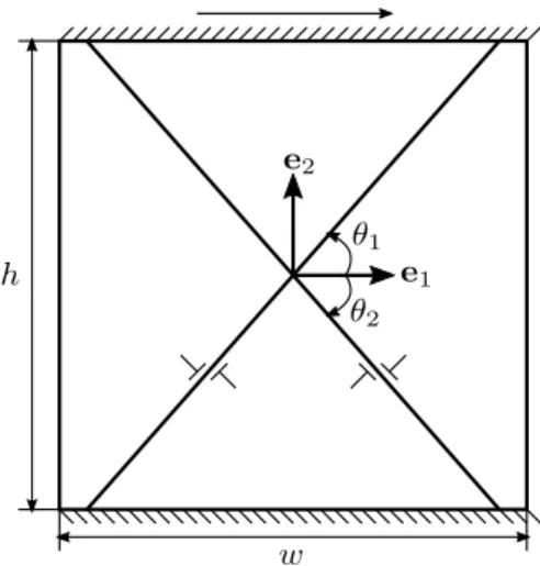
Gurtin et al.,2007;Nellemann et al.,2017). A 2D crystalline strip of height hand widthw is considered, with two active slip systems symmetrically oriented with respect to e₁ direction (θ1 = −θ2 = 60°), as illustrated in Fig. 1. This strip is discretized using 100quadratic finite elements, which represents a good compromise between results accuracy and computation cost. To model the infinite length of the strip ine₁

Fig. 1. 2D crystalline strip with two active slip systems, symmetrically tilted byθ1 = 60° andθ2 = −60° with respect toe₁ direction, for shear test simulations.

direction, the following periodic conditions are imposed on the left and right edges:

ui(0, x2, t) =ui(w, x2, t), fori= 1,2

γ^α(0, x2, t) =γ^α(w, x2, t), forα= 1, 2 (74) In addition, the bottom edge is subject to macro-clamped displacement boundary conditions and the top edge is subject to a loading-unloading cycle of displacement ine₁direction:

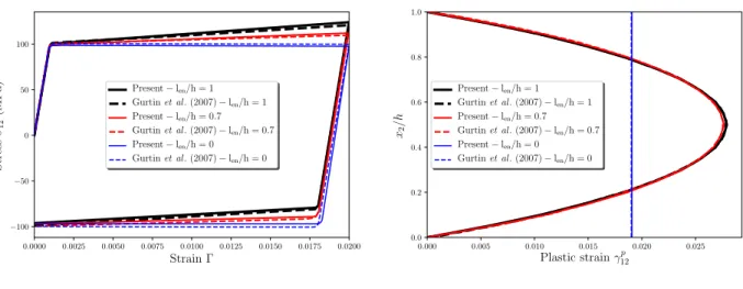
u1(x1,0, t) =u2(x1,0, t) = 0, u1(x1, h, t) =hΓ (t), andu2(x1, h, t) = 0 (75) where Γ (t) is the prescribed shear strain, going from 0to 0.02 and back to 0. In order to establish pro- portional and non-proportional loading conditions, which are necessary to better investigate certain SGCP aspects, two types of microscopic (slip) boundary conditions are also considered on the top and bottom edges. In the case of proportional loading, both the edges are passivated from the beginning to the end of the simulation:

γ^α(x1,0, t) =γ^α(x1, h, t) = 0, forα= 1,2 (76) However, in the case of non-proportional loading, only the bottom edge is passivated over the entire simu- lation. The top edge is assumed to be unpassivated until a certain value of the prescribed shear strain in the plastic range (Γ = 0.01) and then passivated until the end of the simulation:

γ^α(x1,0, t) = 0, γ˙^α(x1, h, t > t0) = 0, forα = 1,2 (77) where t0 is the passivation time, i.e., time at which Γ (t0) = 0.01. Note that, in the considered case of non-proportional loading, nonuniform plastic strain distribution develops within the strip before the non- proportional loading source (top edge passivation) occurs. As will be seen later, this allows for a more complete investigation of the higher-order energetic and dissipative effects under non-proportional loading conditions.

Results in terms of macroscopic stress-strain curves and plastic shear strain distributions ine₂direction are adopted to investigate the influence of the major constitutive parameters on the global response of the considered material, with a focus on those implied in the definition of the higher-order energetic and dissipa- tive stresses. The stress-strain curves are generated based on the average shear stress within the strip (simply notedσ12hereafter) as a function of the prescribed shear strainΓ. For the plastic shear strain distribution in