This is an author-deposited version published in: https://sam.ensam.eu Handle ID: .http://hdl.handle.net/10985/8707
To cite this version :
Dieudonné TSATCHA, Eric SAUX, Christophe CLARAMUNT - A bidirectional path-finding algorithm and data structure for maritime routing - International Journal of Geographical Information Science - Vol. 28, n°7, p.1355-1377 - 2014
Any correspondence concerning this service should be sent to the repository Administrator : [email protected]
Maritime Routing
(Received 00 Month 200x; final version received 00 Month 200x)
Route planning is an important problem for many real time applications in open and complex environments. The maritime domain is a relevant example of such environments where dynamic phenomena and navigation constraints generate dif- ficult route finding problems. This paper develops a spatial data structure that sup- ports the search for an optimal route between two locations while minimizing a cost function. Although various search algorithms have been so far proposed (e.g.
breadth-first search, bidirectional breadth-first search, Dijkstra’s algorithm, A∗, etc.), this approach provides a bidirectional dynamic routing algorithm which is based on hexagonal meshes and an Iterative Deepening A∗algorithm(IDA∗), and a front to front strategy using a dynamic graph that facilitates data accessibility. The whole approach is applied to the context of maritime navigation, taking into account nav- igation hazards and restricted areas. The algorithm developed searches for optimal routes while minimizing distance and computational time.
Keywords:Maritime routing, computational geometry, artificial intelligence, geographic information science, navigation aids.
1. Introduction
Route planning between two geographical positions in a dynamic and open environment is of- ten a frustrating problem for maritime navigation. As the number of entities and rules in these environments increase, path-finding problems are often non straightforward. Several success- ful algorithms developed for Intelligent Transportation Systems (ITS) have been applied to terrestrial environment where path-finding algorithms are network constrained. This is exem- plified by in-vehicle Route Guidance System (RGS) and real time Automated Vehicle Dispatch- ing System (AVDS) where routing strategies rely on road networks. Maritime environment also needs efficient algorithms to find the shortest path from an origin to a destination. But while predefined tracks exist for tankers or large ships, the maritime environment remains an open space where navigation in any direction is allowed, this making the path-finding problem a rather different issue than in network environments.
The challenge considered in this paper is to perform a real-time path-search where a given path is continuously constrained by the objects and the phenomena that are likely to modify the environment and the navigation. The real-time decision process to develop should be com- puted in a few seconds, this being sufficient to take into account possible environment changes (e.g. modification of visibility (fog, night), perception of ships or drifting objects) and to sup-
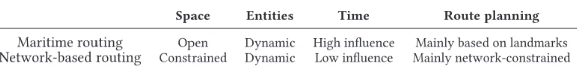
port collision avoidance. Such a path-finding search should also take into account the specific properties of the maritime environment. Table 1 summarizes the main differences between maritime and network-based routing. Navigation in a maritime environment is constrained by several properties such as rules (e.g. traffic regulation, collision regulations (U.S. Coast Guard 1999)), restricted areas (e.g. traffic separation zones or lines), hazard areas (e.g. shoals), mobile objects (e.g. ships) and change dynamically with tide, current and wind. Moreover, visibility which is not constant (e.g., fog, day vs. night) can influence the perception of entities and ac- tions to perform (Tsatchaet al.2013). All these constraints have an impact on the resources, both on computational time and memory space, and penalize real time path-finding.
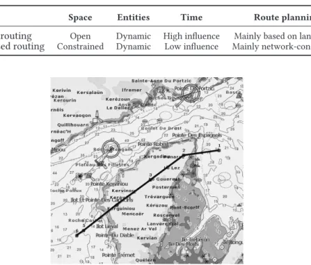
Nowadays, and to the best of our knowledge, Electronic Chart Display and Information Sys- tems (ECDIS) used for maritime navigation integrate some path-finding algorithms as men- tioned by Xuet al.(1994) and Yuet al. (2003). However, none of them take into account all the constraints previously described. Current maritime routing algorithms are usually applied to ship races and take into account meteorologic phenomena (wind, current) on top of raster data (Ahmadiet al.2008). Figure 1 shows an example of a route proposed by MaxSea1 soft- ware where the two most important factors involved in achieving optimum courses are the weather forecast and the speed of the boat. However, this approach does not preserve security and cannot be considered as real time routing.
Table 1. Main differences between maritime and network-based routing.
Space Entities Time Route planning
Maritime routing Open Dynamic High influence Mainly based on landmarks Network-based routing Constrained Dynamic Low influence Mainly network-constrained
Figure 1. Example of a maritime route (black straight line) derived by MaxSea software that crosses a land area.
The approach presented in this paper is oriented to a navigation decision-aid system that should facilitate the decision-process of a captain in high stress situations by proposing an efficient path to follow. Let us first restrict the study to a real time path-finding problem ap- plied to a two-dimensional maritime environment (i.e., 2D map) by taking into account both the length of the trajectory and the static objects composing a region. The choice of a planar
1http://www.maxsea.com
representation rather than an ellipsoidal representation is motivated by the area of navigation that is rather of the size of a region (i.e. coastal navigation) than of the size of a part of the Earth (i.e. off-shore navigation, less constrained by the environment). The maritime environment is modelled by S57 vector data1(format defined by the International Hydrographic Organization (IHO)). In order to achieve planning tasks, most of current maritime transport systems super- impose a grid over a region, and a graph is used to find the best paths. Usually, the terrain is modelled by regular squares (or tiles), hexes or octiles defining the mesh (Yap 2002). However, the number of cells in the path, as well as computational time, can be reduced in the search process using an iterative approach. In order to do so, let us introduce an iterative bidirectional path-finding algorithm based on an optimal graph structuring a hexagonal mesh. The search algorithm is founded on an Iterative Deepening A∗algorithm(IDA∗).
The remainder of the paper is organized as follows. Section 2 introduces the main approaches or algorithms used in path-finding strategies and suggests the more relevant type of mesh for maritime routing. Section 3 introduces the background theory used to built two complementary meshes associated to the bidirectional path and proposes an optimized data structure for storing the hexagonal cells. Section 4 develops the approach retained to merge theIDA∗ algorithm and the bidirectional strategy for hexes and presents a case study. Finally, section 5 draws some conclusions and highlights future work.
2. Path-Finding Algorithms
Two classes of algorithms are usually applied to find an optimal path connecting two points denoteds(starting point) andt(terminal point): unidirectional and bidirectional algorithms.
Each of them has many variants but the most useful algorithms are admissible algorithms. A search algorithm is admissible if it guarantees to find a valid solution that satisfies a minimal path among the set of existent solutions.
Moore (1957) and Dijsktra (1959) algorithms are commonly considered as the first admissible algorithms. Let us consider a mesh (i.e. a partition of the search area into cells) related to a directed graphG(X, U)whereX is a collection of nodes (i.e. cells) andU is a collection of arcs. Each arc ofU can be considered as an ordered pair of nodes ofX. Starting with a node n0 including initial points and for each iteration, the algorithm explores some parts of the graph2 and marks the best successor of the current node until to reach the ending nodenN that includes terminal pointt. A path can be defined by a sub-graph ofGwhere the selected nodes ofXcan be arranged in increasing number and where the initial noden0is assumed to be the root node. A pathustarting from root noden0 to an ending nodenN is denoted as a sequence of arcs, such as:
u= (en0n1, en1n2, en2n3, en3n4, en4n5, . . . , enN−1nN)
wheres∈n0,t∈nN andenk−1nkis the arc formed by the nodesnk−1andnk. Alternatively, one can write:
u= (n0, n1, n2, n3, n4, ..., nN).
The length of the path is computed using the distancel, i.e. : l(u) =PN−1
i=0 ||enini+1||, where||.||is theL2norm.
1http://www.iho.int/iho_pubs/IHO_Download.htm
2In the conceptualization developed, a graph is related to a mesh. A directed graphG(X, U)whereXis a collection of nodes and Uis a collection of arcs. Each arc ofUmay be considered as an ordered pair of nodes ofX.
The best successornj of current nodeni minimizes the distance l(ni, nj) +λn0,ni where l(ni, nj) is the cost between nodesni andnj, and λn0,ni is the minimal cost to reach node ni starting from n0. Dijkstra’s algorithm has been extended into a more efficient algorithm denoted A∗ by including the estimated remaining cost to reach the final node nN. A∗ es- timates the optimal cost of a current node ni with an evaluation function having the form f(ni) =g(ni) +h(ni), whereg(ni)is the cost of the finding path fromn0toni, andh(ni)is a heuristic estimating the cost of the remaining path to reachnN fromni.A∗ is admissible and never overestimates the cost functionfat each iteration in comparison with algorithms which estimate the cost function at the end of the process. It has an iterative variant method denoted
“Iterative DeepeningA∗”(IDA∗)proposed by Korf (1985) where the search is performed by a depth analysis in the graph.
All admissible algorithms can be applied by a bidirectional approach. The bidirectional al- gorithms belong to the second class of algorithms. The aim is to find the optimal path using a heuristic in both directions denoted “forward front” and “backward front” originated from starting noden0 and ending node nN. A Bidirectional Heuristic Pohl A∗ search (BHP A∗) was proposed by Pohl (1971). It was later improved by Kwa (1989) who proposed a Bidirec- tional SearchA∗ (BSA∗) by adding several specific operations (nipping, pruning, trimming (removing) and screening (not placing)). The interest of these operations is to avoid unneces- sary explorations and prevent repeated expansions in both fronts (Pulidoet al.2012). However, these two heuristics have a crucial drawback called missile metaphor (where the two searches pass without touching each other) due to the fact that they perform a heuristic with the prin- ciple front-to-end1. In comparison withBHP A∗ andBSA∗, Sint and de Champeaux (1977) and de Champeaux (1983) proposed a front-to-front2principle. Kaindl and Kainz (1997) show that the front-to-front evaluations are more efficient than the front-to-end evaluations. In the 90’s, Dillenburg and Nelson (1994) and Manzini (1995) introduced an approach in comparison with the bidirectional search called perimeter search. This approach is based on a front-to-front strategy using a breadth-first search and generates nodes around the evaluated node and stores all of them located within a research area limited by a boundary. Later, Kaindl and Kainz (1997) devised an algorithm computationally cheaper than the previous ones that relies on dynamic changes called difference approaches. This approach is grounded on a known costg(ni)and its heuristic estimates the cost from a given evaluation functionh(ni) which minimizes the estimations obtained with other heuristics.
Cui and Shi (2011) show that the sort of grid used can have an impact on the performance of path-finding algorithms. Sahret al. (2003) and Tong et al. (2013) introduce relevant dis- crete global grid systems (DGGSs) which are considered to be a promising structure for global geospatial information representation based on hexagonal grids. Having the objectives to find an optimal path in real-time in a maritime environment, we propose a routing algorithm based on a front-to-front Bidirectional Iterative DepthA∗algorithm (BIDA∗). The bidirectional al- gorithm is dynamic and develops a non overlapping mesh paving part of the maritime envi- ronment.
Hexagonal mesh performs the three main factors usually used to evaluate a graph search on a grid:
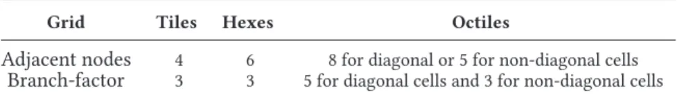
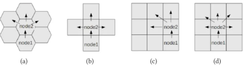
(1) It minimizes the branch-factor value3 defined by Korf (1985). This criterion is illus- trated in figures 2(a), 2(b), 2(c), 2(d) and summarized in table 2.
1Evaluations estimate the minimal cost of some paths from an evaluated nodenito the terminal nodenN.
2Evaluations estimate the minimal cost of some paths from an evaluated nodeniin the forward front to nodenjof the backward front.
3The branch-factor value is the number of possible adjacent nodes in order to avoid backtrack.
(2) It minimizes the number of nodes contained in the solution path. According to Yap (2002), this path minimizes the number of changes in direction.
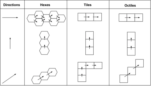
(3) It proposes an optimal cluster movement (Yousefi and Donohue 2004). This criterion enables to determine the longest node sequence in a direction while minimizing both the direction changes and the total number of nodes composing the path (Figure 3).
Table 2. Number of adjacent nodes and branch-factor value for different grids.
Grid Tiles Hexes Octiles
Adjacent nodes 4 6 8 for diagonal or 5 for non-diagonal cells Branch-factor 3 3 5 for diagonal cells and 3 for non-diagonal cells
These facts have made hexagonal mesh as the optimal method which offers several advan- tages for a grid solution for the navigation planning problem. The next section focuses on the data structure used to implement theBIDA∗algorithm with a hexagonal mesh. TheBIDA∗ algorithm is then detailed in section 4.
(a) (b) (c) (d)
Figure 2. Branch-factor for (a) a hexagonal grid, (b) a square tile grid, (c) an octagonal grid and a non- diagonal cell, (d) an octagonal grid and a diagonal cell.
Figure 3. Optimal cluster movement on different grids.
3. Hexagonal Mesh Path and Data Structure
The aim of this section is to find the directions of propagation in the bidirectional search while producing a complementary mesh for the solution path. This is achieved by a two-step ap- proach. The first step presented in section 3.1 determines the modelling process for a hexagonal mesh. This implies that the hexagonal cells should not overlap when the two paths meet. The second step, detailed in section 3.2, selects the more efficient direction of propagation that min- imizes the constraints required by the application. Finally, section 3.3 proposes a data structure to store the hexagonal cells of the solution path.
3.1. Complementary Hexagonal Mesh
The main principle of this process is based on mesh parallelism applied on the planar faces.
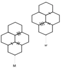
According to Pottmann et al. (2007a), parallelism can be used to produce a unified view or complementary mesh by keeping optimal nodes and the offset of geometrical properties. Let us consider two meshesMandM′displayed in figure 4. These authors prove that these meshes are combinatorially equivalent if and only if there is a 1-1 correspondence between vertices and edges. It follows that two meshesMandM′are considered as parallel since the corresponding edges are parallel (Pottmannet al.2007b).
Figure 4. Example of parallel meshesM andM′with planar faces. Meshes are combinatory equivalent and corresponding edges are parallel.
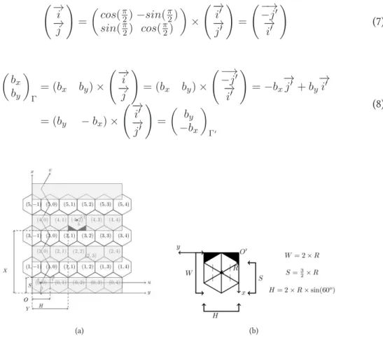
Let us consider two pointssandtin a two-dimensional space corresponding to the starting and terminal points. There always exists a propagation initiated bysthat covers the terminal pointtwith a hexagon. Based on the proof of parallelism between meshes, there exists one and only one hexagon (node) initiated by a centrebthat contains the pointtand whose mesh initiated by itself meets exactly the mesh initiated by the centres. One of the complexities of this algorithm is to compute the coordinates of the centre of the hexagon which covers point tstarting from points. The computation of the centrebis realized assuming the hexagonal mesh to be represented by a two-dimensional fixed matrix where indexesiandj represent the indexes of the columns and rows respectively using zigzag axes (Figure 5(a)). Finding the hexagonal cell that containstis equivalent to find the indexes(i, j)of the hexagonal cell which coverst. The coordinates of this centre are derived from the formulae detailed as follows, where we considerΓ(O,−→
i ,−→
j)being the initial coordinate system of figure 5.
The strategy to compute the centreb= (bx, by)of the hexagon that contains terminal node t= (tx, ty)is realised by a two-step approach. The first step subdivides the space with rect- angular tiles corresponding to a two-dimensional matrix. A tile is identified by its indexes (itile, jtile)and the coordinates of its left-top corner. In figure 5, the widths of the rows and columns are respectively equal toH andS. The second step is to use the indexes of the tile containing the terminal pointtfor determining the indexes (ihex, jhex)of the final hexagon and the coordinates of its centre.
(a) (b)
Figure 5. Schema of a hexagonal mesh (a) in a coordinate systemΓ(O,−→ i ,−→
j)and (b) in a local coordi- nate systemγ(O′,−→u ,−→v).
The indexes(itile, jtile)of the tile that containstare computed by equation 1:
itile =tx
S
jtile =
jt
y
H
k jt
y−H2
H
k
whenitileis odd whenitileis even
=yts
H
withyts =ty−itilemod 2×H2
(1)
In addition, the point tcan be defined in the local coordinate systemγ(O′,−→u ,−→v)associ- ated to the tile that containst(Figure 5(b)). Its local coordinates(tx_tile, ty_tile)are defined by equation 2:
tx_tile=tx−itile×S and ty_tile=yts−jtile×H (2) The next step concerns the identification of the hexagonal cell (among the three possible hexagonal cells that intersect the tile(itile, jtile)) containing the terminal pointt. This point belongs either to the light black area or the dark black one in figure 5(a). The boundary of these two areas is defined by the following equation:
x_tile=R× 1
2 −y_tile H
(3) It results that the indexes(ihex, jhex)of the hexagon that contains pointt(tx, ty)are:
ihex=
(itile whentx_tile> R×
1
2 −ty_Htile itile−1 otherwise
jhex=
(jtile whentx_tile> R×
1
2 −ty_Htile jtile−itilemod2 +d otherwise
withd=
(1 when ty_tile> H2 0 otherwise
(4)
The parameterddifferentiates the case wheretbelongs to the dark black top (d= 0) or dark black bottom (d= 1) hexagon.
Finally, the coordinates of the centre of the hexagon that contains pointtare:
bx=ihex×S+R and by =jhex×H+H2 (5) Centering the reference systemΓto starting pointsby a translation of vector(R,H2)leads to the new coordinates:
bx =ihex×S and by =jhex×H (6) Two kinds of mesh can be distinguished for the paving. One can have a flat (Figure 5(b)) or pointy orientation (Figure 6(b)). The second orientation is derived from the first one by changing the coordinate system. We arbitrary chose this orientation in the following sections.
LetΓ′(s,−→ i′,−→
j′)be this new reference system displayed in figure 6.Γ is derived fromΓ′ by applying a rotation of angle π2 (Equation 7). In this new coordinate system, the point b = (bx, by)is defined by equation 8.
−
→i
−
→j
!
=
cos(π2)−sin(π2) sin(π2) cos(π2)
×
−
→i′
−
→j′
!
=
−→−j′
−
→i′
!
(7)
bx by
Γ
= (bx by)×
−
→i
−
→j
!
= (bx by)×
−→−j′
−
→i′
!
=−bx−→
j′ +by−→ i′
= (by −bx)×
−
→i′
−
→j′
!
= by
−bx
Γ′
(8)
(a) (b)
Figure 6. Schema of a hexagonal mesh in a coordinate systemΓ′(s, i′, j′).
Finally, starting from a hexagonal cell centred on initial points, this modelling process en- ables to compute the centrebof the hex-cell containing the final pointt to be joined while
producing a complementary mesh for the routing problem. The next section focuses on the choices of directions of propagation for the forward and backward fronts in the bidirectional search.
3.2. Directions of Propagation in the Bidirectional Search
This section introduces a real-time dynamic direction finding while avoiding backtracks. A direction of exploration is hereafter denoted as a beam. Assuming a hexagonal mesh, the ob- jective is to determine the set of hexes contained in a beam corresponding to a next possible direction (i.e. the search area) on which theBIDA∗algorithm will be applied. Each searching area is defined with three adjacent hexes whose number corresponds to the value of the branch- factor (see section 2). It results that there exists six beams (three beams and their symmetric) initiated by a hexagonal cell (Figure 7).
(a) (b) (c)
Figure 7. Symmetry in the direction of beams.
Assuming an initial hexagon of centrec, space is partitioned into conic sections(Conei)6i=1 centred on this hexagon. Each conic section, obtained by a rotation of π3 aroundc, contains three adjacent hexes that can be chosen in the path-finding. A conic section is identified by its direction of propagation denotedVibeing the interior bisector.
The solution beams result from a minimisation problem. One has to determine the efficient beams that minimize the criteria required by the application. The navigation or displacements imply to take into account two fundamental types of constraints: spatial and temporal. Each of them can be consistency or requirement constraints. On the one hand, consistency constraints are generic and do not depend on a project or application. They are always related to the intrinsic properties of the entities located in the environment. On the other hand, requirement constraints represent as an example building regulations, best-practise construction rules, or client requirements, which may vary from the applications (Borrmannet al.2009). Therefore, let us consider(cs, ct)i the pair of spatial and temporal constraints restricted to the beami.
The challenge of the computational algorithm is to find the beam which satisfies the set of constraints or minimizes the functions modelling these constraints. Regarding the temporal constraint satisfaction problem, Schwalb and Vila (1998) define it like a computational solution to represent and perform queries on temporal occurrences and relations.
Borrmannet al.(2009) distinguishes three different types of spatial constraints: distance con- straint (distance, closerThan, fartherThan and maxDist), directional constraints (above, below, northOf, southOf, eastOf, westOf) and topological constraints (disjoint, meet, overlap, cover, coveredBy, contain, equal and inside). This section explores directional constraints and the next section 4 dedicated toBIDA∗satisfies the distance and topological constraints. The di- rectional constraint is expressed as to be as close as possible to the directionD=−−→
bibj defined from the straight line joining the centresbi andbj of the cells associated to the forward and backward fronts (see figure 8). The bidirectional process leads to use symmetrical beams on both parts of the propagation. Thus, optimal directionV¯i minimizes the criterion defined by equation 9:
(D, V\¯i) =Mini=1...6(D, V\i) (9)
Figure 8. Symmetrical propagation using complementary beams.
3.3. Data Structure
This section develops an optimized data structure to implement theBIDA∗algorithm taking into account the issue of memory consumption. This implies that the data structure should en- able to store the two oriented beams of the bidirectional search. This latter should be dynamic, including relationships linking a parent hexagon to a sequence a neighbouring child cells. The process should also be optimized with the objective that the coordinates of each hexagon and corresponding vertices must be computed only once. The proposed data structure is modelled as two separated dynamic oriented and complementary graphs where the root nodes are the hexagons that contain initial pointssandtand whose the centre coordinates are defined by section 3.1. Two nodes are joined by one direction or arc (parent-child). We derive the following notations regarding the relations between two neighbouring nodes:
Rpc:parent-child relation Rcp:child-parent relation
Rpbb:brother-brother relation having parentp
(10)
The data structure allows to build and store hexagons by a dynamic process. Figure 9 shows that the hexagonal mesh can be organised from global or local points of view. According to an absolute reference system, a hexagon is identified with its row and column indexes(i, j)as explained in section 3.1. As regards a local reference system centred on a current hexagon, six child hexagons are placed on different directions(N E, E, SE, SO, O, N O)identified asViin the previous section:N Eis denoted by 1,Eby 2,SEby 3,SOby 4,Oby 5 andN Oby 6. In the absolute reference system, relations between indexes (row, column) of two neighbouring nodes exist. Assuming the variation(δi,δj)din directiondfrom a node(i, j)to a node(i′, j′), indexes can be computed using equation 11. Table 3 identifies the variation coefficients associated with the possible directions.
(i′, j′) = [−1]i(δi, δj)d+ (i, j) (11)
(a) (b)
Figure 9. Modelling of neighbouring cells in a local (left) or global (right) reference system.
Table 3. Variation coefficients between parent and child.
d 1 2 3 4 5 6
(δi,δj)d (−1,0) (−1,1) (0,1) (1,1) (1,0) (0,−1)
A hexagonal cell(i, j)is defined in the graph from the following notation:
mn[Hex(i, j)]dSpc
dpc: direction parent-child of the current cell from the parent point of view
(i, j): indexes of the current hexagon (row, column) m, n: left and right directions bordering directiondpc
S: set of directions identifying the children
(12)
In figure 9(b), the graph node related to the cell(i−1, j)is denoted as62[Hex(i−1, j)]16,1,2. Directionsm = 6,dpc = 1andn = 2are defined from the indexes(i, j) of the parent cell and correspond to a beam having a directionV1illustrated by figure 7(c) (right configuration).
Directions in setS = {6,1,2}are defined from the indexes(i−1, j)of the current cell and identify the possible neighbouring cells(i−2, j),(i−2, j+ 1)and(i−1, j+ 1)extending the structure. Considering the definition of a hexagonal mesh in any directions and at the same resolution, the modelling is realized by a growing process. The first step is the modelling of the root cell(i, j)(Figure 10). To start with, the cell(i, j) is assimilated to a point. It can be either the starting pointsor the centre of the hexagon containing the terminal pointt. Rotating around the centre of the cell enables to update the set of children stored in set S. At the end of this process the data structure is restricted to a single root cell denoted as00[Hex(i, j)]01,2,3,4,5,6. By convention, a null direction(m= 0,dpc= 0orn= 0)implies that the cell has no parent.
Figure 10. Illustration of the root cell modelling process.
The second step consists in the creation of the six child cells of the initial or root cell. This step defines the first ring around an initial hexagon (Figure 11). In order to optimize the data structure, the brother-brother relationsRpbbbetween the children are updated. The graph dis- played in figure 12 shows the data structure associated to the first ring of cells where the cell (i, j)is the root node. Each arc is oriented from a child to its parent and labelled with the di- rectiondcp. The directiondcpis not only used in order to label the arcs in the graphs of figures
12 and 14 but also to update the child nodes in S of the parent cell. It can be derived that if a child node “looks” its parent in directiondcpthen the parent “looks” its child in the direction dpcdefined by equation 13:
dpc= (dcp+ 2)mod6 + 1 (13)
Figure 11. Illustration of the first ring modelling process.
Figure 12. Graph corresponding to the structure of figure 11.
Applying the previous process to the following child cells leads to the second ring mod- elling process illustrated by figure 13 and corresponding graph presented in figure 14. Starting from the first child cell62[Hi−1,j]16,2,1 three child cells are built in directions 6, 1 and 2 (Fig- ure 13(a)). This leads to the definition of cells51[H(i−2, j)]65,6,1,62[H(i−2, j+ 1)]16,1,2 and
13[H(i−1, j+ 1)]21,2,3 (Figure 14). These new cells are considered as the children of the cur- rent cell(i−1, j)that implies to update the brother relationsRbbp between the new three cells and the older ones (i.e. to update the relations between brothers(i, j+ 1),(i−1, j+ 1)and brothers(i−1, j−1),(i−2, j)). The bordering new brothers to update are indicated by the indexesmandnin the cell notation. This implies to create a link between the brothers identi- fied by directionsmand(m+ 4)mod6 + 1(according to the current cell(i−1, j)) as well as the brothers identified by directionsnandnmod6 + 1. In the previous example, setS of cell (i, j+ 1)is modified to include its new brother in its direction 1. Thus, number 1 is removed from S and cell(i, j+ 1)becomes13[H(i, j+ 1)]22,3(Figure 14). The same principle is applied to cell(i−1, j−1)whereSis modified to include its new brother in its direction 1. Thus, number 1 is removed from S and cell(i−1, j−1)becomes51[H(i−1, j−1)]65,6(Figure 14). This pro- cess is repeated on the next child cells of the root cell (see figures 13(b),13(c),13(d),13(e),13(f)) and ends the second ring. Next iterations are based on the same principle. The resulting data structure is optimized in the sense that there is no graph node duplication and that node links are computed once.
(a) (b) (c) (d)
(e) (f)
Figure 13. Illustration of the second ring modelling process.
Figure 14. Graph corresponding to the structure of figure 13(a).
The previous data structure has been presented from a general context and for a whole mesh.
Using a direction of propagation like defined in figure 7 of section 3.2 limits the number of computation and produces a sub-graph of the proposed one. This reduces the computation cost and provides an optimal data structure to apply the bidirectional iterative path-finding algorithm.
From a computational and visualisation point of view, two neighbouring cells are joined by two common vertices. Assuming the vertices(vi)6i=1of a hexagon (wherev1is the vertex at the top of a hex-cell) and in order to avoid repeated vertex calculations, each directionViis linked to the vertexviin the hexagonal cell. In figure 15, the rotation around the centre of the hexagon (i, j)in direction(Vi)6i=1leads to the creation of the six verticesvi. Each of these vertices are common to the parent cell(i, j)and two of its child cells. For each hexagonal cell, a hash table stores all the vertices previously computed avoiding redundant vertex computations in the mesh and optimizing the visualisation process. The hash table is updated taking into account the mesh generation process. As an example and after the creation of the root cell(i, j)(Figure 15), the vertexv2belongs to the three cells(i, j),(i−1, j)and(i, j+ 1)and a neighbouring
cell(i−1, j)has its two verticesv4andv5already built (hash table view per line). Centred on a cell and analysing the hash table, one deduces the vertices not yet defined and their direction of construction.
Figure 15. Hash table illustrating the vertex computations of the hexagon during the creation of the root cell(i, j).
4. BIDA∗ on Hexes
4.1. Bidirectional Path-Finding based onIDA∗
The complexity of search algorithms is usually considered in terms of time, space and cost of the solution path.IDA∗is known to be asymptotically optimal in these three dimensions for exponential tree searches (Korf 1985). This latter can be efficiently combined with bidirectional search andIDA∗ is the only known algorithm that is able to find an optimal solution when practical resources are limited. Dantzig (1960) initially proposed the bidirectional algorithm and an interpretation as follows: “If the problem is to determine the shortest path from a given origin to a given destination, the number of comparisons can often be reduced in practice by fanning out from both the origin and the destination, as if they were two separate independent problems. . . . However, once the shortest path between a node and the origin or the destination is found in one problem, the path is conceptually replaced by a single arc in the other problem.” Nicholson (1966) and Dreyfus (1969) proposed many approaches to improve this previous description. From this interpretation, Korf (1985) derives that bidirectional search optimizes space and time by search- ing simultaneously forward from the initial state and backward from the goal state, and storing the states generated until a common one is found on both search frontiers. Table 4 summarizes the cost of theIDA∗ algorithm with different grids (Yap 2002). The hexagonal mesh offers a good compromise between the length of the path and the complexity. Assuming that a hashing schema and hexagonal mesh are used, it results that the complexity of bidirectional algorithm in time and space isO(2.42D−H2 ).
Table 4. Complexity ofIDA∗according to different grids (Yap 2002).
D =l(u)andHcorresponds to the effect of the heuristic on the algo- rithm.
Grid Tiles Hexes Octiles
Average depth 1.00D 0.81D 0.71D
IDA∗complexity 0(3.00D−H) 0(2.42D−H) 0(2.77D−H)
The principle ofIDA∗is as follows. For each iteration, a Depth-First Search(DF S)is real- ized to find the next node in the graph. TheDF Sexplores the three possible nodes in a beam
cutting the branches when the value of the cost functionf(ni) = g(ni) +h(ni) exceeds a threshold value. The cost functionf(ni)considers that g(ni)is the cost of the finding path fromsto ni, andh(ni)is a heuristic estimating the cost of the remaining path fromni to t.
The threshold value used for an iteration is the minimum cost value among all the possible cost values at the previous iteration. The idea of this algorithm is not to minimize the depth search, but rather to minimize the total cost of the path (i.e. functionf). An example of node selection is illustrated by figures 16, 17 and 18. Our algorithm restricted to a search direction constrained by beams does not counteract the admissibility property ofIDA∗algorithm.
Figure 16. An initial graph with cost values. Figure 17. The solution path.
Figure 18. Node selection (in dark grey) usingIDA∗.
The algorithm presented in appendix A provides the main concepts used in the implemen- tation ofBIDA∗ for the case studies presented in section 4.2.M aprepresents the set of ge- ographical features used for the maritime environment. Two threadsT1 andT2 have been applied in parallel for the bidirectional search.(tip)causes the current thread to suspend its execution for a specified period avoiding concurrent processing. Each thread is related to a dynamic data structure of search denoted asM eshi(i= 1,2)where a mesh is a set of hexag- onal cells as defined by equation 12. At each step of the hexagon cell creation, a nodeN(i,j) corresponds to a vertex and can be assimilated to a row of the hash table (see figure15). In order to avoid a redundant process, each mesh is managed by two stacks of nodes. The first stack of nodes is a set of promising nodes to explore and evaluate using a functionf =g+h, denoted as open stack (Stack1).Stack1has a LIFO1 architecture. The second is a set of visited nodes that are not selected to reach the goal and is denoted as closed stack of nodes (Stack2). The
1Last-in, First-out
radius of the hexagonal cells is linked to parameterr. It ensures either a fine or large resolu- tion of the solution path. Two approaches can be taken into account. On the one hand,rcan be invariant during the path-finding algorithm as presented in figure 20 ensuring a single level of resolution. On the other hand, a multi-resolution approach can be used where a discrete grid system is represented by a group (aperture) of 3, 4 or 7 hexagons (Sahr 2011). All these apertures preserve the centre of the current cell but its radius can change allowing to refine or enlarge the resolution dynamically. Three parameters enable the change of resolution of hexagonal cells: i) centrecii) radiusrand iii) deviation angleαcomputed between the symmetrical axes of two consecutive resolutions. Thus, one can determine the properties (i.e.r′,c′andα′) of a hexagonal grid at a lower resolution from the parameters at a higher one (i.e.r,candα). In aperture 4, the parameters are computed as follows:r′= 2∗r,c′ =candα = 0. Figure 19 is an example ofBIDA∗ algorithm with such a multi-resolution approach applied on an aperture 4. The main drawback encountered using a multi-resolution strategy is that it counteracts the complementarity conditions (see section 3.1) between the two directional paths, i.e. the two last cells of each directional path intersect.
4.2. BIDA∗for Maritime Routing
TheBIDA∗algorithm has been applied to maritime data to find the optimal route joining two positions corresponding to the departure and arrival points of a ship trajectory. In order to find an optimal route, one should take into account two constraints. The first one is to avoid hazard areas during routing while taking into account meteorological and environmental information such as wind and current. The second one is to consider the semantic information generated by a region or an object (e.g. cardinal buoy, alignment) that can modify the trajectory ship. In order to avoid hazard areas and for each iteration of theBIDA∗algorithm, let us compute the spatial relationships (equal, disjoint, intersect, touch, cross, within, contain, overlap (Freeman 1975)) between a cell(i, j)in the mesh and the different objects forming the maritime environment.
If an intersection exists, the search tries to find an other solution path among the brother cells (see section 3.3). In the case where no solution is found among the “brothers”, the strategy is to have a backward process. One comes back to the “father” cell in order to find a solution among its brothers. In the case study, the cost functiong (respectivelyh) evaluates the Manhattan distance between the starting (respectively ending1) and the current point.
The approach has been applied to maritime data extracted from Electronic Navigational Charts (ENC). These charts are defined from vector files where geographic objects are mod- elled using geometrical primitives like point, line, polygon defined in the European Datum 1950 (ED50) geodetic datum. The S572 format describes the concepts of the maritime environment with their attributes. The proposed example uses electronic chart number 7066 provided by the SHOM3 (“Service Hydrographique et Océanographique de la Marine”, Brest, France) and represents a maritime area in the surrounding area of Brest city in France.
The user first submits departure points, destination pointtand the radius of the hexagonal cells. The cell radius can be arbitrary set for computational time purpose (large radius reduces computational time) or having a meaning for the application like being a safety or security area around the ship related to a minimal distance and defined according to the speed and rate of turn4of the ship.
1In the bidirectional algorithm, the ending point does not correspond to the terminal pointtbut to the centre of the front node in the symmetrical path.
2http://www.iho.int/iho_pubs/IHO_Download.htm
3http://www.shom.fr
4ROT attribute in the Automated Identification System (AIS) format.
Figures 19 and 20 respectively illustrate the results using a multi-resolution and a single resolution hexagonal mesh. In our case study, the relevant cells of the bidirectional path are displayed satisfying the heuristic function while avoiding the hazard areas like land areas (light grey areas), buoys (light grey circles) and restricted areas (dark grey areas). The sea area is rep- resented by a white colour. The prototype was implemented in Java language using the Java topology suite (JTS5) for representing the spatial relationships. The black line illustrates the proposed route and the hexagonal cells correspond to the graph nodes deployed for this so- lution. Each node of the graph builds exactly three children. The three black nodes in figure 19 are the children of the current nodes in the forward and backward fronts. Table 5 pro- poses some results to evaluate the performance of the strategy. The criteria hereafter used are the ratioγ quantifying the gain of nodes in the ordinary path-finding problem and the computational time. The ratio γ evaluates the number of cells required in the proposed al- gorithm in comparison with the number of cells needed for covering the whole search space (N bhexagon = Surface of the search space
Surface of a hexagon ). As an example, the ratioγ1of the first use case in table 5 is equal to142177−1014
142177 = 0.99. This means that only1%of the cells of a coverage grid is needed to compute the optimal solution. Computational time presented in the last column of table 5 has been obtained by a computer with an Intel Celeron Processor E3200 (2.40 GHz). One can remark that this strategy minimizes the processing time by optimizing the storage of nodes.
This is especially true in large and open environnments.
Figure 19. Example of iterative maritime routing using theBIDA∗algorithm on a dynamic data struc- ture. Case 1: multi-resolution hexagonal meshes with an aperture 4.
Table 5. Evaluation of the proposed strategy in comparison with a usual strategy based on a coverage grid.
Departure point s(km)
Destination point t(km)
Radius of a hexagon (m)
Number of cells in the graph
Number of cells mesh- ing the environment
Number of cells in the solution path
γ Computational
time (ms)
-524282.64 5379318.29
-497390.83 5382653.57
50 1014 142177 338 0.99 21350
-524282.64 5379318.29
-510401.87 5377558.01
50 576 142177 172 0.99 8207
-524313.63 5379102.12
-497019.12 5382653.57
96 567 38568 185 0.98 5309
-524313.63 5379102.12
-497019.12 5382653.57
122 432 23881 144 0.98 5332
-524313.63 5379102.12
-497297.90 5385000.62
150 558 15798 159 0.96 11477
-505228.18 5375396.25
-497297.90 5385000.62
103 240 15798 80 0.98 2969
5http://www.vividsolutions.com/jts/jtshome.htm
Figure 20. Example of maritime routing solution (black line) using theBIDA∗algorithm on a dynamic data structure. Case 2: single resolution hexagonal mesh.
5. Conclusion
This paper introduces a spatial data structure applied to a real-time path-finding algorithm in open maritime environments. It is based on a hexagonal mesh and a dynamic data structure.
This data structure is applied to aBIDA∗ algorithm in order to derive an optimal track in terms of distance and complexity. The proposed data structure has several properties that (i) determine a complementary hexagonal mesh producing a complete paving for the solution path and (ii) optimize the direction of propagation by following one of the three directions required by the branch-factor. This latter is implemented on a dynamic and hierarchical graph avoiding the duplication of graph nodes and the redundancy of information in the nodes. Furthermore, this data structure reduces computational time and memory space costs of the solution path that is relevant for real-time path-finding. In the context of real-time maritime navigation, one can use a bidirectional path-finding to have real-time foresights of the route to follow.
Accordingly, the real-time track process can facilitate captain decision making during high stress or workload situations. A direction for future research is to integrate additional maritime navigation constraints like weather, meteorological information and the semantics generated by entities or other mobile objects around the ship (Tsatchaet al.2013). All these constraints could further improve the proposed safety track.
Acknowledgements
The authors acknowledge the three anonymous referees for their detailed and valuable com- ments which have improved this paper. We are also grateful to the SHOM (“Service Hydro- graphique et Océanographique de la Marine”, Brest, France) for their maritime data and support in this research.
References
Ahmadi, S., Ebadi, H., and Valadan, Z., 2008. A new method for path finding of power trans- mission lines in geospatial information system using raster networks and minimum of mean algorithm.World Applied Sciences Journal, 3 (2), 269–277.
Borrmann, A., Hyvärinen, J., and Rank, E., 2009. Spatial Constraints in Collaborative Design Processes.In:Proceedings of the International Conference on Intelligent Computing in Engi- neering (ICE’09). Berlin, Germany, Berlin, Germany.
Cui, X. and Shi, H., 2011. A*-based pathfinding in modern computer games.International Jour- nal of Computer Science and Network Security (JCSNS), 11 (1), 125–130.
Dantzig, G.B., 1960. On the shortest route through a network.Management Science, 6 (2), 187–
190.
de Champeaux, D., 1983. Bidirectional heuristic search again.Journal of the ACM (JACM), 30 (1), 22–32.
Dijsktra, E.W., 1959. A note on two problems in connexion with graphs.Numerische Mathe- matik, 1 (1), 269–271.
Dillenburg, J.F. and Nelson, P.C., 1994. Perimeter search.Artificial Intelligence, 65 (1), 165–178.
Dreyfus, D., 1969. An appraisal of some shortest-path algorithms.Operations research, 17 (3), 395–412.
Freeman, J., 1975. The modelling of spatial relations.Computer Graphics and Image Processing, 4 (2), 156–171.
Kaindl, H. and Kainz, G., 1997. Bidirectional heuristic search reconsidered.Journal of Artificial Intelligence Research, 7, 283–317.
Korf, R.E., 1985. Iterative-deepening-A: an optimal admissible tree search.In:Proceedings of the 9th International Joint Conference on Artificial Intelligence (IJCAI’85), Vol. 2 Morgan Kauf- mann Publishers Inc., San Francisco, CA, USA, 1034–1036.
Kwa, J.B., 1989. BS*: an admissible bidirectional staged heuristic search algorithm.Artificial Intelligence, 38 (1), 95–109.
Manzini, G., 1995. BIDA*: an improved perimeter search algorithm.Artificial Intelligence, 75 (2), 347–360.
Moore, E., 1957. The shortest path through a maze.In:Proceedings of the International Sympo- sium on Theory of Switching CambridgeHarvard University Press.
Nicholson, T.A.J., 1966. Finding the shortest route between two points in a network.The Com- puter Journal, 9 (3), 275–280.
Pohl, I., 1971. Bi-directional search.In: Meltzer and Michie, eds.Machine Intelligence., Vol. 6 Edinburgh University Press, 127–140.
Pottmann, H., Brell-Cokcan, S., and Wallner, J., 2007a. Discrete surfaces for architectural design.
In: P. Chenin, T. Lyche and L.L. Schumaker, eds.Curves and Surfaces: Avignon 2006. Nashboro Press.
Pottmann, H.,et al., 2007b. Geometry of multi-layer freeform structures for architecture.ACM Transactions on Graphics - Proceedings of ACM SIGGRAPH 2007, 26 (3), article No. 65.
Pulido, F.J., Mandow, L., and Pérez de la Cruz, J.L., 2012. A two-phase bidirectionnal heuristic search algorithm.In:Proceedings of the Sixth Starting AI Researcher’s Symposium (STAIRS), 240–251.
Sahr, K., 2011. Hexagonal discrete global grid systems for geospatial computing.Archives of Photogrammetry, Cartography and Remote Sensing, 22, 363–376.
Sahr, K., White, D., and Kimerling, J.A., 2003. Geodesic discrete global grid systems.Cartography and Geographic Information Science, 30 (2), 121–134.
Schwalb, E. and Vila, L., 1998. Temporal constraints: a survey.Constraints, 3 (2-3), 129–149.
Sint, L. and de Champeaux, D., April 1977. An improved bidirectional heuristic search algo- rithm.Journal of the ACM (JACM), 24 (2), 177–191.
Tong, X.,et al., 2013. Efficient encoding and spatial operation scheme for aperture 4 hexagonal discrete global grid system.International Journal of Geographical Information Science, 27 (5), 898–921.
Tsatcha, D., Saux, E., and Claramunt, C., 2013. A modeling approach for the extraction of se- mantic information from a maritime corpus. Advances in Geographic Information Science, In: S. Timpf and P. Laube, eds.Advances in Spatial Data Handling. Springer Berlin Heidelberg, 175–191.
U.S. Coast Guard, 1999.Navigation rules: international-inland. Technical report, U.S. Depart- ment of Transportation, United States Coast Guard, 2100 Second St., SW Washington, DC 20593-0001.
Xu, J., Lathrop, J., and G., R., 1994. Improving cost-path tracing in a raster data format.Com- puters & Geosciences., 20 (10), 1455–1465.
Yap, P., 2002. Grid-based path-finding.In:Proceedings of the 15th Conference of the Canadian Society for Computational Studies of Intelligence on Advances in Artificial Intelligence, 44–45.
Yousefi, A. and Donohue, G.L., 2004. Temporal and spatial distribution of airspace complexity for air traffic controller workload-based sectorization.In:Proceedings of the 4th American In- stitute of Aeronautics and Astronautics (AIAA) Aviation Technology, Integration and Operations Forum, Chicago, IL.
Yu, C., Lee, J., and Munro-Stasuik, M.J., 2003. Extensions to least-cost path algorithms for road- way planning.International Journal of Geographical Information Science, 17 (4), 361–376.
Appendix A. Maritime Path-Finding Algorithm based onBIDA∗
AlgorithmA.1:
Input Starting pointsand terminal pointt: two geographical positions.
1: r: the radius of a hexagonal cell.
2: M ap: the set of geographical features representing the environment.
Output P ath: the set of nodes (i.e. vertex and its indexes) defining the solution path.
3: functionBIDA∗(s, t, r, M ap) ⊲The main bidirectional path-finding function based on two threads.
4: M esh1, M esh2, Stack11, Stack12, Stack21, Stack22, P ath1, P ath2←∅
5: Cell, P node←∅
6: ObstacleArea←selectF eaturesF romM ap(M ap) ⊲This procedure selects the features/objects to avoid during the navigation (e.g. restricted areas, hazard areas, buoys, etc.).
7: whilejoinM eshes(M esh1, M esh2)6=truedo
8: if currentT hread() =T1then
9: Cell←updateM esh(T1, s, t, r, M esh1, Stack11, Stack12, M esh2)
10: P node←parentN ode(Cell)
11: P ath1←P ath1∪P node
12: wait(tip)
13: else ifcurrentT hread() =T2then
14: Cell←updateM esh(T2, s, t, r, M esh2, Stack21, Stack22, M esh1)
15: P node←parentN ode(Cell) ⊲Update the indexes.
16: P ath2←P ath2∪P node
17: wait(tip)
18: end if
19: end while
20: P ath←mergingP ath(P ath1, P ath2)
21: returnP ath ⊲Return the optimal path.
22: end function
Input Tj: the thread to process.
23: sandt: two geographical positions.
24: r: the radius of a hexagonal cell.
Input and
Output M eshj: a directional mesh.
25: Stack1: the stack of selected nodes for the solution path.
26: Stack2: the stack of visited nodes and evaluated using functionf =g+h. The best promising node is at the top of the stack.
27: functionupdateM esh(Tj, s, t, r, M eshj, Stack1, Stack2, M eshi) ⊲This procedure returns the best cell inM eshjin the path-finding search and updates the outputs.
28: Cell←∅
29: ifM eshj=∅then
30: ifcurrentT hread() =T1then
31: N(0,0)←buildF irstN ode(s, r) ⊲ sis the centre of the first cell andN(0,0)is the first node of the forward front (Figure 11).
32: else
33: N(0,0)←buildLastN ode(s, t, r)⊲The function computes the centrebof the last node using the formula presented in section 3.1 and generates the first node of the backward front.
34: end if
35: pushStack(N(0,0), Stack2)⊲Put the first node at the top of the stack of the visited nodes.
36: else
37: ifStack26=∅then
38: N(i,j)←popStack(Stack2) ⊲This function selects the best node at the top of the stack.
39: ifpositionSelected(N(i,j), Stack1) =true)then ⊲This function checks if node N(i,j)corresponds to a geographical position or space that has already been selected and stored in Stack1
40: return∅
41: end if
42: if(meetObstacle(N(i,j), ObstacleArea) =true)then
43: return∅
44: else
45: P artialCell←extractRelationsF romM esh(M eshj, N(i,j)) ⊲Centred on N(i,j), the function extracts the set of vertices (and their relations) already built inM eshj. For the first nodeN(0,0), this function only computes the first hexagonal cell00[Hex(0,0)]01,2,3,4,5,6.
46: Cell←buildCell(P artialCell, N(i,j), M eshj) ⊲Computes the cell associated toN(i,j)from PartialCell and its complementary (i.e. the vertices ofN(i,j)not yet defined) (Figure 15).
47: storeCell(Cell, M eshj)
48: V¯i←optimalDirection(M eshj, M eshi)
49: Beam←generateT hreeBestN odes(Cell, V¯i)
50: pushStack(sort(Beam), Stack2)
51: pushStack(N(i,j), Stack1)
52: returnCell
53: end if
54: end if
55: end if
56: end function