HAL Id: tel-01202442
https://hal.archives-ouvertes.fr/tel-01202442
Submitted on 21 Sep 2015HAL is a multi-disciplinary open access archive for the deposit and dissemination of sci-entific research documents, whether they are pub-lished or not. The documents may come from teaching and research institutions in France or abroad, or from public or private research centers.
L’archive ouverte pluridisciplinaire HAL, est destinée au dépôt et à la diffusion de documents scientifiques de niveau recherche, publiés ou non, émanant des établissements d’enseignement et de recherche français ou étrangers, des laboratoires publics ou privés.
Dynamic observers and system control, application to
large scale systems
Nan Gao
To cite this version:
Nan Gao. Dynamic observers and system control, application to large scale systems. Automatic. Université de Lorraine, 2015. English. �tel-01202442�
D´epartement de Formation Doctorale en Automatique Ecole doctorale IAEM Lorraine´ UFR Sciences et Technologies
Observateurs dynamiques et
commande des syst`
emes, application
aux syst`
emes de grande dimension
TH`
ESE
pr´esent´ee et soutenue publiquement le 29 juin 2015 pour l’obtention du
Doctorat de l’Universit´
e de Lorraine
(Sp´ecialit´e Automatique, Traitement du signal et des images, G´enie informatique) par
Nan GAO
Composition du jury
Pr´esident : Mohammed M’SAAD Professeur, ´Ecole Nationale Sup´erieure d’Ing´enieurs de Caen
Rapporteurs : Olivier SENAME Professeur, Grenoble INP
Driss BOUTAT Professeur, INSA Centre Val de Loire
Examinateurs : Holger VOOS Professeur, Universit´e du Luxembourg
Marouane ALMA Maˆıtre de conf´erence, Universit´e de Lorraine
Directeur de th`ese : Mohamed DAROUACH Professeur, Universit´e de Lorraine
Acknowledgments
My deepest gratitude goes first and foremost to Prof. Mohamed Darouach, my supervisor, for his constant encouragement and guidance. Three years ago, it was my first time to go abroad alone and study in a new environment. Prof. Darouach gave me bunches of advice and helped me conquer many difficulties in both my study and my life. I offer my sincere appreciation and gratitude to his patient advice and warm help.
I would like to thank all the members of my PhD evaluation committee: Prof. Olivier Sename, from Grenoble INP, Prof. Driss Boutat, from INSA Centre Val de Loire, Prof. Holger Voos, from University of Luxembourg, Prof. Mohammed M’saad, from ENSICAEN, Dr. Marouane Alma, from University of Lorrain. I am very grateful to all of them for spending their valuable time to read and review carefully my thesis.
I would also like to thank other staffs of CRAN-Longwy: Michel Zasadzinski, Latifa-Boutat-Baddas, Harouna Souley Ali, Mohamed Boutayeb, Hugues Rafaralahy, Cèdric Delattre, Joëlle Pinelli and Nathalie Clèment, for helping me a lot with many issues.
I wish to express my gratitude to all the PhD students whom I have encountered during the past three years: Gloria Lilia Osorio Gordillo, Hao Nguyen Dang, Yassine Boukal, Florian Seve, Titif Matchbetikh, Adrien Drouot, Ghazi Bel Haj Frej, Bessem Bhiri, and Asma Barbata, who have instructed and helped me a lot in the past three years.
I wish to express my heartfelt gratitude to my parents, Shuntong GAO and Yulian YUAN, and all the other family members. As your single son, I know how hard for you to be apart with me. Thank you for consistently encouraging me to be brave, independent and optimistic, and I appreciate your support and love in these years.
Finally, but not lastly, I am grateful to my wife, Peng LI, for the happy and hard time together during our study in these ten years. Thank you very much for your understanding, patience, and help. I am so happy to grow up with you.
Contents
Acknowledgments i
Notation and acronyms ix
List of Figures xi
Chapter 1 Introduction
1.1 Introduction . . . 2
1.2 Observers for linear systems . . . 5
1.2.1 Full-order observers and observer-based control . . . 5
1.2.2 Reduced-order observers . . . 7
1.2.3 Functional observers . . . 8
1.2.4 Unknown input observers . . . 10
1.2.5 Observers for uncertain systems . . . 12
1.2.6 H∞observers . . . 14
1.2.7 Proportional integral observers . . . 15
1.2.8 Dynamic observers . . . 18
1.3 Large scale system and decentralized observers . . . 20
1.3.1 Large-scale system . . . 20
1.3.2 Decentralized observers . . . 22
Contents
1.4.1 Controllability and Stabilizability . . . 24
1.4.2 Observability and Detectability . . . 25
1.4.3 Schur complement lemma . . . 25
1.4.4 Lyapunov stability of linear systems . . . 26
1.4.5 Bounded real lemma . . . 26
1.5 Structure of the thesis . . . 27
Chapter 2 New H∞dynamic observer design 29 2.1 Introduction . . . 30
2.2 A new H∞dynamic observer design for continuous-time systems . . . 30
2.2.1 Observer design for systems without disturbances . . . 32
2.2.2 Parameterization of algebraic constraints . . . 34
2.2.3 Observer design for systems in the presence of disturbances . . . 42
2.2.4 Particular cases . . . 46
2.2.5 Numerical example . . . 48
2.3 A new H∞dynamic observer design for discrete-time systems . . . 58
2.3.1 Observer design for systems without disturbances . . . 59
2.3.2 Parameterization of algebraic constraints . . . 61
2.3.3 Observer design for systems in the presence of disturbances . . . 64
2.3.4 Particular cases . . . 68
2.3.5 Numerical example . . . 70
2.4 A new H∞dynamic observer design for uncertain systems . . . 76
2.5 Conclusions . . . 83
Chapter 3 H∞dynamic-observer-based control design 85 3.1 Introduction . . . 86
3.2 Problem formulation . . . 86
3.3 Algebraic constraints and parameterizations . . . 87
3.3.1 Algebraic constraints . . . 87
3.3.2 Parameterizations . . . 90
3.4 H∞dynamic-observer-based control design . . . 93
3.5 Numerical example . . . 97
3.5.1 Observer-based control design . . . 98
3.5.2 Simulation results . . . 99
Chapter 4
H∞decentralized dynamic-observer-based control for large-scale uncertain systems103
4.1 Introduction . . . 104
4.2 Problem formulation . . . 104
4.3 Algebraic constraints and parameterizations . . . 107
4.3.1 Algebraic constraints . . . 107
4.3.2 Parameterizations . . . 110
4.4 H∞decentralized dynamic-observer-based control design . . . 113
4.5 Numerical example . . . 118
4.5.1 Observer-based control design . . . 120
4.5.2 Simulation results . . . 121
4.6 Conclusions . . . 127
Chapter 5 Conclusions and perspectives 129 5.1 Conclusions . . . 130
5.2 Perspectives . . . 130 Appendix A
Publication list 133
Notation and acronyms
Sets and Norms
Rn Set of n-dimensional real vectors Rn×m Set of n×m dimensional real matrices
Fc Field of complex numbers
�.�2 The Euclidean vector norm
�.�∞ The H∞norm
Re(λ) The real part of eigenvalue λ
Matrices and Operators
A > 0 Real symmetric positive-definite matrix A I Identity matrix of appropriate dimension In Identity matrix of dimension n × n
0 Null matrix of appropriate dimension
0n Null matrix of dimension n × n
A−1 Inverse of matrix A ∈ Rn×n, det A �= 0
AT Transpose of matrix A
A⊥ Any matrix such that A⊥A = 0 and A⊥A⊥T > 0 A+ Generalized inverse of matrix A satisfying AA+A = A
(�) Block induced by symmetry
rank A Rank of matrix A
Notation and acronyms
Acronyms
BMI Bilinear Matrix inequality
DGCS Decentralized Guaranteed Cost Stabilization
DO Dynamic Observer
HDO H∞dynamic observer
IGBT Insulated Gate Bipolar Transistor
LMI Linear Matrix Inequality
LSM Linear Stepping Motor
LSS Large-scale System
LTI Linear Time Invariant
LTV Linear Time Varying
PO Proportional Observer
PI Proportional Integral
PID Proportional Integral Derivative PIO Proportional Integral Observer
SISO Single-input Single-output
T-S Takagi-Sugeno
List of Figures
1.1 VX2600 High Precision DC Source . . . 3
1.2 ADA4870 Package . . . 3
1.3 Structure of observer . . . 4
1.4 Electric Power System . . . 20
1.5 Large-Scale System . . . 21
2.1 Control input . . . 50
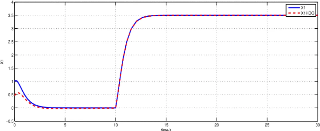
2.2 State x1 and its estimate (solid line: original state; dashed line: estimate) . . . . 51
2.3 Estimation error e1 . . . 51
2.4 State x2 and its estimate (solid line: original state; dashed line: estimate) . . . . 51
2.5 Estimation error e2 . . . 52
2.6 State x3 and its estimate (solid line: original state; dashed line: estimate) . . . . 52
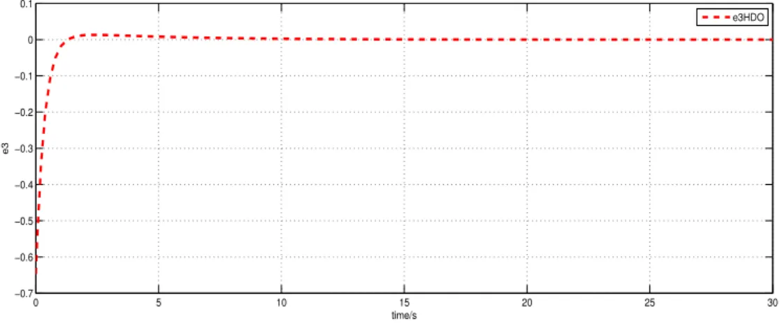
2.7 Estimation error e3 . . . 52
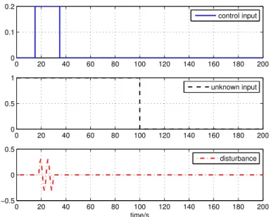
2.8 All inputs (solid line: control input; dashed line: unknown input; dash-dotted line: disturbance) . . . 53
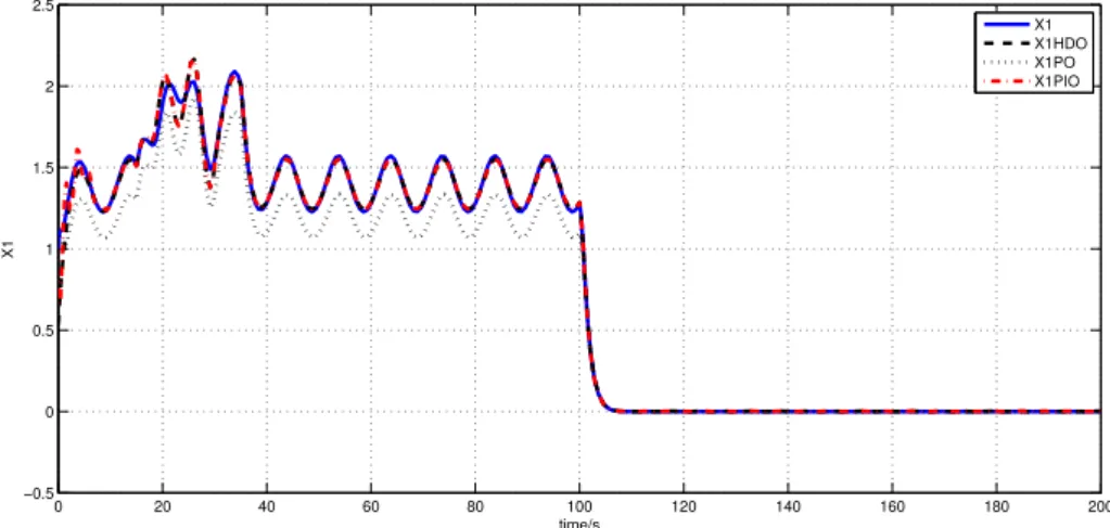
2.9 State x1 and its estimates for 200s (solid line: original state; dashed line: HDO; dotted line: PO; dash-dotted line: PIO) . . . 54
2.10 State x1 and its estimates for 40s (solid line: original state; dashed line: HDO; dotted line: PO; dash-dotted line: PIO) . . . 54
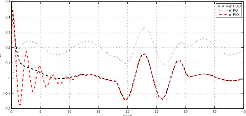
2.11 Estimation error e1 for 200s (dashed line: HDO; dotted line: PO; dash-dotted line: PIO) . . . 54
2.12 Estimation error e1for 40s (dashed line: HDO; dotted line: PO; dash-dotted line: PIO) . . . 55
2.13 State x2 and its estimates for 200s (solid line: original state; dashed line: HDO; dotted line: PO; dash-dotted line: PIO) . . . 55
2.14 State x2 and its estimates for 40s (solid line: original state; dashed line: HDO; dotted line: PO; dash-dotted line: PIO) . . . 55
List of Figures
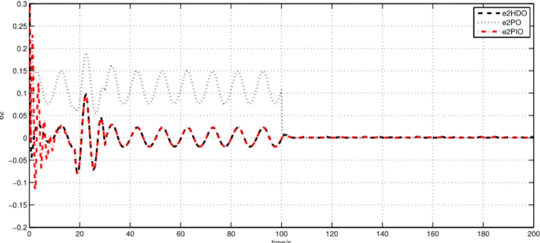
2.15 Estimation error e2 for 200s (dashed line: HDO; dotted line: PO; dash-dotted
line: PIO) . . . 56
2.16 Estimation error e2 for 40s (dashed line: HDO; dotted line: PO; dash-dotted line: PIO) . . . 56
2.17 State x3 and its estimates for 200s (solid line: original state; dashed line: HDO; dotted line: PO; dash-dotted line: PIO) . . . 56
2.18 State x3 and its estimates for 40s (solid line: original state; dashed line: HDO; dotted line: PO; dash-dotted line: PIO) . . . 57
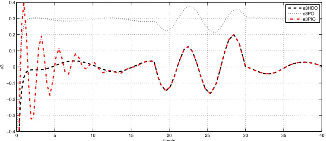
2.19 Estimation error e3 for 200s (dashed line: HDO; dotted line: PO; dash-dotted line: PIO) . . . 57
2.20 Estimation error e3 for 40s (dashed line: HDO; dotted line: PO; dash-dotted line: PIO) . . . 57
2.21 All inputs (dashed line: unknown input; dash-dotted line: disturbance) . . . 73
2.22 State x1 and its estimates for 5s (solid line: original state; dashed line: HDO; dotted line: PO; dash-dotted line: PIO) . . . 73
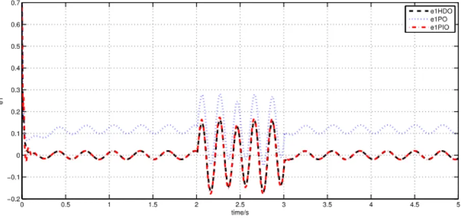
2.23 Estimation error e1 for 5s (dashed line: HDO; dotted line: PO; dash-dotted line: PIO) . . . 73
2.24 Estimation error e1 for 1s (dashed line: HDO; dotted line: PO; dash-dotted line: PIO) . . . 74
2.25 State x2 and its estimates for 5s (solid line: original state; dashed line: HDO; dotted line: PO; dash-dotted line: PIO) . . . 74
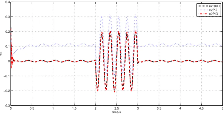
2.26 Estimation error e2 for 5s (dashed line: HDO; dotted line: PO; dash-dotted line: PIO) . . . 74
2.27 Estimation error e2 for 1s (dashed line: HDO; dotted line: PO; dash-dotted line: PIO) . . . 75
2.28 State x3 and its estimates for 5s (solid line: original state; dashed line: HDO; dotted line: PO; dash-dotted line: PIO) . . . 75
2.29 Estimation error e3 for 5s (dashed line: HDO; dotted line: PO; dash-dotted line: PIO) . . . 75
2.30 Estimation error e3 for 1s (dashed line: HDO; dotted line: PO; dash-dotted line: PIO) . . . 76
3.1 Disturbance . . . 99
3.2 State x1 and its estimate (solid line: original state; dotted line: HDO) . . . 100
3.3 Estimation error e1 . . . 100
3.4 State x2 and its estimate (solid line: original state; dotted line: HDO) . . . 100
3.5 Estimation error e2 . . . 101
3.6 State x3 and its estimate (solid line: original state; dotted line: HDO) . . . 101
3.7 Estimation error e3 . . . 101
3.8 Output y . . . 102
4.1 Disturbances . . . 122
4.2 State x11and its estimate (solid line: original state; dotted line: HDO) . . . 122
4.3 Estimation error e11 . . . 123
4.4 State x12and its estimate (solid line: original state; dotted line: HDO) . . . 123
4.5 Estimation error e12 . . . 123
4.6 State x13and its estimate (solid line: original state; dotted line: HDO) . . . 124
4.8 State x21and its estimate (solid line: original state; dotted line: HDO) . . . 124
4.9 Estimation error e21 . . . 125
4.10 State x22and its estimate (solid line: original state; dotted line: HDO) . . . 125
4.11 Estimation error e22 . . . 125
4.12 Output y1 . . . 126
CHAPTER
1
Introduction
Contents
1.1 Introduction . . . . 2
1.2 Observers for linear systems . . . . 5
1.2.1 Full-order observers and observer-based control . . . 5
1.2.2 Reduced-order observers . . . 7
1.2.3 Functional observers . . . 8
1.2.4 Unknown input observers . . . 10
1.2.5 Observers for uncertain systems . . . 12
1.2.6 H∞observers . . . 14
1.2.7 Proportional integral observers . . . 15
1.2.8 Dynamic observers . . . 18
1.3 Large scale system and decentralized observers . . . 20
1.3.1 Large-scale system . . . 20
1.3.2 Decentralized observers . . . 22
1.4 Background . . . 24
1.4.1 Controllability and Stabilizability . . . 24
1.4.2 Observability and Detectability . . . 25
1.4.3 Schur complement lemma . . . 25
1.4.4 Lyapunov stability of linear systems . . . 26
1.4.5 Bounded real lemma . . . 26
Chapter 1. Introduction
1.1 Introduction
The focus of this dissertation is to develop and design a new class of observers called dynamic observer (DO) and to use it in control design. In the past several decades, the observer design problem has gained constantly high interest in the literature, due to the fact that the state vari-able cannot be measured frequently either because of the unavailability of appropriate sensors or due to high costs and long analysis times involved in the measurement processes.
The state variable is important in the state space representation, which is a mathematical model of a physical system as a set of inputs, outputs and state variables related by first-order differ-ential equations. The general state space representation of linear continuous-time systems is expressed as
˙x = Ax + Bu, (1.1a)
y = Cx + Du, (1.1b)
where x ∈ Rn, u ∈ Rmand y ∈ Rp are the state vector, the input vector and the output vector,
respectively. Matrices A, B, C and D are known constant and of appropriate dimensions. The state space representation of linear discrete-time systems is expressed as
x(k + 1) = Ax(k) + Bu(k), (1.2a)
y(k) = Cx(k) + Du(k), (1.2b)
where x(k) ∈ Rn, u(k) ∈ Rmand y(k) ∈ Rpare the state vector, the input vector and the output
vector, respectively.
In the state space representation, the state variable can show the full characteristics of system, therefore it is widely applied in the control process, such as state feedback control ([53] and [110]). State feedback control is to place the closed-loop poles of a system in the pre-determined locations of complex plane, by controlling the system state.
Take system (1.1) for example. The state feedback control law is represented by
u = Ksfx, (1.3)
where Ksf is unknown matrix and of appropriate dimension to be determined.
By inserting state feedback control (1.3) into system (1.1a) it follows that:
˙x = (A + BKsf)x. (1.4)
In this case, the gain matrix Ksf can be derived from the solution of the following equation:
A + BKsf = Fsf, (1.5)
where Fsf represents the matrix of the pre-determined location of system poles.
Although state variables are of great importance, most of the time, state variables are not all available due to the package technology, or costly and difficulty to measure. Take the precision power source VX2600 for example. The VX2600 is a high precision DC source of VX Instruments company. The output voltage and current of VX2600 are ±10VDC and ±5mADC, respectively.
In order to guarantee the accuracy of precision source, it must be packaged in a sealed box so that to isolate the outside disturbance. In this case, it is impossible to measure the states of some internal variables directly.
1.1. Introduction Even if the source is not packaged in a black box, it is still difficult to measure the states. Let us see the following figure of VX2600:
Figure 1.1: VX2600 High Precision DC Source
One can see from Figure 1.1 that VX2600 is made up of many electronic elements, such as capacitors, resistors, digital chips and so on. With the development of manufacture technology, now the digital chips can be made as small as possible. For example, the distance between two pins of chip ADA4870 is 1.27 millimeters, as shown in Figure 1.2. In this case, it is difficult to measure the value of one pin without touching other pins.
Figure 1.2: ADA4870 Package
On the other hand, the sensors and their associated cables are among the most expensive com-ponents in the system. The accuracy of sensors also reduces the reliability of control procedure, since sensors usually produce errors, such as noise and limited responsiveness.
Chapter 1. Introduction
With all the above discussions, it is necessary to use the observer to estimate the state in the case where the state cannot be determined by direct measurement. The concept of observer was firstly introduced by D.G. Luenberger [80] and [81], based on the theory that a system S2 is
served as an observer of the system S1if the available inputs and outputs of system S1 are used
as inputs to drive system S2.
In control theory, an observer is a dynamic system that reconstructs the state of a given real system, from the measurements of inputs and outputs of the real system. Let us consider the following system:
˙x = Ax + Bu, (1.6a)
y = Cx. (1.6b)
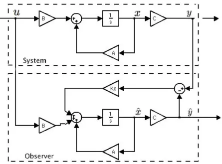
For system (1.6), an observer is given by
˙ˆx = Aˆx + Bu + Ko(y− ˆy), (1.7a)
ˆ
y = C ˆx, (1.7b)
where ˆx ∈ Rn is the state of observer, called also the state estimate. ˆy ∈ Rp is the output of
observer. Ko is an unknown gain matrix and of appropriate dimension be determined.
One can see from system (1.7) more clearly that the observer is a reconstruction of the system states by using the inputs and outputs of original system. The only difference is that there is an additional term Ko(y− ˆy) in the observer, which is used to ensure that the state estimate ˆx
converges to the system state x, on receiving successive measured values of system inputs and outputs.
The structure of observer (1.7) is shown in the following figure:
1.2. Observers for linear systems
1.2 Observers for linear systems
Ever since Luenburger presented the first result on the observer, the observers design have been greatly investigated and widely applied for linear systems (see [21,43,52,61,123] and references therein). The observer aims to estimate the system state x. Therefore we must study the estimation error e (e = ˆx−x). From system (1.6) and observer (1.7), we obtain the following estimation error dynamic:
˙e = ˙ˆx − ˙x,
= Aˆx + Bu + Ko(y− ˆy) − Ax − Bu,
= (A− KoC)ˆx− (A − KoC)x,
= (A− KoC)e. (1.8)
By using Lyapunov function approach, we can determine the parameter matrix Ko such that
system (1.8) is asymptotically stable, i.e, e → 0 when t → ∞. In this case, system (1.7) is an asymptotic observer for system (1.6).
The observer can be designed for either a continuous-time system or a discrete-time system. The characteristics are the same, and the design processes are at least very similar and in some cases they are identical. For the continuous-time system, the observer is asymptotically stable when the system matrix “A − KoC” has all the eigenvalues on the left side of complex plane, while
for the discrete-time system the observer is asymptotically stable when the system matrix has all the eigenvalues inside the unit circle.
1.2.1 Full-order observers and observer-based control
1.2.1.1 Full-order observers
During the past several years, many kinds of observers have been developed. One popularly used is the full-order observer [41]. Let us consider observer (1.7) for example. Notice that the dimension of observer state ˆx is n, which is equal to the order of original system state. We call this kind of observers full-order observers, which can estimate all the system states.
A full-order observer accomplishes the estimation purpose by calculating the residual “(y − ˆy)”, which is the difference between the measured output and the corresponding quantity generated by the observer. In real world there are many formulations of observers, and most of them can be transformed into observer (1.7). For example, for system (1.6), the author of [82] proposed the following observer:
˙ˆx = ˆAˆx + Ly + Hu, (1.9a)
ˆ
y = C ˆx. (1.9b)
Matrices ˆA, L and H are unknown and of appropriate dimensions to be determined. Notice that if we take
ˆ
A = A− KoC,
L = Ko,
H = B, we can obtain the form of observer (1.7).
Chapter 1. Introduction
The applications of full-order observer can be found in many fields. For example, a distributed full-order observer type consensus protocol was proposed for inear multi-agent systems in [73]. In [82], the author designed a full-order observer for the state estimation of an aircraft motion. The authors of [36] and [97] solved the design problem of full-order observers for sensorless induction motor drives. In [124], a full-order observer based insulated gate bipolar transistor (IGBT) temperature estimation was presented.
1.2.1.2 Observer-based control
As it is discussed previously, the appearance of observer is due to the importance of system states in the feedback control, which is the most important among the various applications of observers. In the case where some states cannot be measured directly, we use their estimates in the control process, which is called observer-based control.
The observer-based control algorithm is designed in two parts: a “full-state feedback” part based on the assumption that all the state variables can be measured; and an observer to estimate the state of the process. The concept of separating the control design into these two parts is known as the separation principle, which is often a practical solution to many design problems.
Take system (1.6) for example, let us consider the following observer-based control law:
u = Kcx,ˆ (1.10)
where Kcis the control gain matrix of appropriate dimension to be determined.
By inserting control (1.10) into system (1.6), we obtain ˙x = Ax + BKcx,ˆ
= Ax + BKc(ˆx− x) + BKcx,
= (A + BKc)x + BKce. (1.11)
From equations (1.8) and (1.11), we obtain the following system:
˙η = Acη, (1.12) where η = � x e � , Ac = � A + BKc BKc 0 A− KoC � . Then we can determine matrices Kcand Koseparately.
In the past decades, the observer-based control has been introduced into many fields. In [78], the authors investigated the problem of observer-based control for linear systems with limited communication capacity. The separation theorem for robust pole placement of discrete-time linear control systems with full-order observers was derived in [114]. The authors of [117] introduced an observer-based control approach for linear stepping motor (LSM) drive systems. In [129], the observer-driven switching stabilization problem for a class of switched linear sys-tems was solved. The paper [142] concerned the problem of event-driven observer-based feed-back control for linear systems. Other applications of observer-based control can be found in [103,105,150] and references therein.
1.2. Observers for linear systems
1.2.2 Reduced-order observers
Generally, in many systems, some state variables can be either measured directly, or calculated from the output. For system (1.6) we can see that in equation (1.6b), system output y has a relation with system state x, i.e.,
y = Cx.
In this case, we can calculate some system states and it is not needed to estimate all the system states. Instead, by taking “y = Cx” into account, one just needs to design an observer to estimate the unmeasured states. This kind of observer, which has lower dimension than the original system or the full-order observer, is called the reduced-order observer [80].
In order to design the reduced-order observer, we should perform some matrix transformations first [122]. For system (1.6), assume that C is a full rank matrix, that is, rank C = p. Then select a (n − p) × n matrix R such that the following n × n matrix P is nonsingular:
P = � C R � . (1.13) Let x = P−1x, where x is a new state variable, then we obtain
A = P AP−1 = � A11 A12 A21 A22 � , B = P B = � B1 B2 � , C = CP−1=�Ip 0�,
In this case, from system (1.6) we obtain the following equivalent system: � ˙x1 ˙x2 � = � A11 A12 A21 A22 � � x1 x2 � + � B1 B2 � u, (1.14a) y = �Ip 0 ��x1 x2 � = x1. (1.14b)
One can see from equation (1.14b) that state x1can be obtained from output y and we just need
to design an observer for the following system of dimension n − p:
˙x2 = A21x1+ A22x2+ B2u (1.15)
The observer for system (1.15) is given by
˙z = (A22+ LA12)z + [(A22+ LA12)L + A21+ LA11]y + (B2+ LB1)u, (1.16a)
ˆ
x2 = z− Ly, (1.16b)
where z ∈ Rn−p is the state of observer and ˆx2 ∈ Rn−p is the estimate of x2. L is the observer
gain matrix and of appropriate dimension to be determined such that: lim
Chapter 1. Introduction
By using this method, the authors of [130] proposed a type of reduced-order observer for matrix second-order linear systems. In [147], the design problem of positive real control via reduced-order observer was solved. The applications of this method can be also found in [143], [151] and references therein.
Another method to design the reduced-order observer is a direct one without doing the trans-formation to original system. For system (1.6), the authors of [64] proposed the following reduced-order observer:
˙z(t) = Dz(t) + Gu(t) + Hy(t), (1.17a)
ˆ
x(t) = M z(t) + N y(t), (1.17b)
with the observer vector z ∈ Rn−p. Matrices D ∈ R(n−p)×(n−p), G ∈ R(n−p)×m, H ∈ R(n−p)×p,
M ∈ Rn×(n−p)and N ∈ Rn×p are unknown to be determined. In this case, one can determine
all the matrices through the analysis of estimation error dynamic directly.
The applications of this method can be found in [50] where the reduced-order observer was designed for rectangular descriptor systems and in [131] where the problem of reduced-order-observer-based decentralized guaranteed cost stabilization (DGCS) of large systems was ad-dressed.
Remark 1.2.1. From the above results, we can see that the minimum order of reduced-order ob-server is n − p, which is a necessary condition of the existence of reduced-order obob-server.
1.2.3 Functional observers
The design problem of a linear functional observer has gain considerable attention recently. Lin-ear functional observers estimate linLin-ear functions of states without estimating all the individual states. Such functional estimates are useful in feedback control system. It is often that a state feedback control law does not necessarily require the availability of the complete states. Take control (1.3) for example. One can see that the control
u = Ksfx
is a linear function of state variables.
Furthermore, in the process of fault detection via residual signal generation, only the estimate of the output is required (y), which is a linear function of states (y = Cx). In this case, it is more logical to estimate the desired output directly using a functional observer rather than estimating all the individual states.
The functional observer is essentially a reduced-order observer, because we only estimate a desired linear function of states by using functional observer. Besides, it can be seen that the condition for the existence of the functional observer is weaker than the detectability condition which is required in full- and reduced-order observers design.
Generally, in order to solve the functional observer design problem, many authors have proposed to transform the initial system to an equivalent one (by using some regular transformations) of reduced-order and to design an observer for this system. Recently, a straightforward method for functional observer design has been developed in [25]. For example, let us consider the following linear system:
˙x = Ax + Bu, (1.18a)
y = Cx, (1.18b)
1.2. Observers for linear systems where zf ∈ Rr is the vector to be estimated with r ≤ n. Matrix Lf is known constant and of
appropriate dimension. Without loss of generality, we assume that rank C = p and rank Lf = r.
For system (1.18), the functional observer is given by
˙
wf = Nfwf + Jfy + Hfu, (1.19a)
ˆ
zf = wf + Efy, (1.19b)
where wf ∈ Rr is the state of functional observer and ˆzf is the estimate of zf. Matrices Nf, Jf,
Hf and Ef are unknown and of appropriate dimensions to be designed.
In this case, we have the following results on the estimation error:
ef = ˆzf − zf,
= wf + EfCx− Lfx,
= wf − Pfx, (1.20)
where Pf = Lf − EfC.
From equation (1.20), we obtain the dynamic of estimation error ef:
˙ef = w˙f− Pf˙x,
= Nfwf + Jfy + Hfu− PfAx− PfBu,
= Nf(wf − Pfx) + (NfPf + JfC− PfA)x + (Hf − PfB)u,
= Nfef + (NfPf + JfC− PfA)x + (Hf − PfB)u. (1.21)
Notice that if the following conditions are satisfied:
NfPf + JfC− PfA = 0, (1.22a)
Hf = PfB, (1.22b)
the dynamic of estimation error ef becomes
˙ef = Nfef. (1.23)
By using Lyapunov function approach to make matrix Nf to be a Hurwitz, ˆzf is an asymptotic
estimate of the linear functional zf for any x(0), w(0) and u(0). The design problem of the
func-tional observer (1.19) is reduced to determine all the parameter matrices such that conditions (1.22) are satisfied and matrix Nf is Hurwitz.
The applications of this approach can be found in many fields. The paper [29] concerned the design of functional observers for linear time-invariant (LTI) descriptor systems. The minimum order linear functional observer was designed in [40]. In [100], a finite time functional ob-server was proposed for linear systems. The authors of [101] designed a single linear functional observer for LTI systems.
Chapter 1. Introduction
1.2.4 Unknown input observers
In the observer design problem, it is necessary to estimate the state of systems in the presence of completely unknown inputs. This kind of observers, which are able to estimate the state of systems in the presence of unknown inputs, is called unknown input observer (UIO).
One method to design UIO depends on the matrix transformation [70,99,121]. The main step of this approach is to find a transformation to decompose the system in two subsystems. In one subsystem, the states are not effected by the unknown input and can be reconstructed by using the observer. In the other subsystem, the rest of the state can be expressed by using the system output and the state estimate of the first subsystem.
Let us consider the following linear system in the presence of unknown inputs:
˙x = Ax + Bu + F v, (1.24a)
y = Cx, (1.24b)
with v ∈ Rl is the unknown input. Matrix F is known constant and of appropriate dimension.
We assume that rank C = p, rank F = l and p ≥ l. Under the assumption that rank F = l, we select a matrix N ∈ Rn×(n−l)such that the following matrix is nonsingular:
T =�N F�. (1.25)
Let
x = T�x, where �x is the new state variable, then we obtain
� A = T−1AT = � � A11 A�12 � A21 A�22 � , � B = T−1B = � � B1 � B2 � , � F = T−1F = � 0 I � , � C = CT =�CN CF�. In this case, system (1.24) becomes
˙�x = �Ax + �� Bu + �F v, (1.26a) y = C��x, (1.26b) where states �x = � � x1 � x2 � , �x1 ∈ Rn−land �x2 ∈ Rl.
Furthermore, we select a matrix Q ∈ Rp×(p−l)such that the following matrix is nonsingular:
U =�CF Q�. Then we have the following results:
U−1 = � U1 U2 � ,
1.2. Observers for linear systems
U1CF = Il, (1.27a)
U2CF = 0. (1.27b)
In this case, by using the following output transformation: � y = � � y1 � y2 � , = U−1y, = � U1 U2 �� CN CF�x,� = � U1CN U1CF U2CN U2CF � � � x1 � x2 � , and equations (1.27a) and (1.27b), we obtain
�
y1 = U1y = U1CN�x1+x�2, (1.28)
�
y2 = U2y = U2CN�x1. (1.29)
From equation (1.28) we have the following result on �x2:
�
x2 = U1y− U1CN�x1. (1.30)
By substituting equation (1.30) into system (1.26), we obtain
˙�x1 = A�1�x1+ �B1u + E1y, (1.31a) � y2 = C�1x�1, (1.31b) with � A1 = �A11− �A12U1CN, E1 = �A12U1, � C1= U2CN.
One can see from system (1.31) that state �x1 is not effected by the unknown input v and it can
be reconstructed by using observer (1.7). Besides, state �x2 can be obtained from output y and
state estimate ˆ�x1.
In this case, the complete estimate of original system state can be expressed by
ˆ x = T � ˆ � x1 U1y− U1CN ˆx�1 � . (1.32)
Notice that one should do matrix transformation by using the above method. In order to simply the design procedure, another approach named the algebraic method has been developed. For system (1.24), the authors of [33] proposed the following UIO:
˙z = N z + Ly + Gu, (1.33a)
ˆ
x = z− Ey (1.33b)
where z is the state vector. Matrices N, L, G and E are unknown and of appropriate dimensions to be determined.
Chapter 1. Introduction
In this case, from system (1.24) and UIO (1.33), we obtain the following estimation error dy-namic:
˙e = ˙ˆx − ˙x, = ˙z− P ˙x,
= N (z− P x) + NP x + LCx + Gu − P Ax − P Bu − P F v,
= N e + (N P + LC− P A)x + (G − P B)u − P F v, (1.34) where matrix P = In+ EC.
One can see from equation (1.34) that if the following constraints are satisfied:
N P + LC− P A = 0, (1.35a)
G− P B = 0, (1.35b)
P F = 0, (1.35c)
the estimation error dynamic ˙e will be independent of state x, input u and unknown input v. In this case, the estimation error dynamic becomes
˙e = N e. (1.36)
Then, the design problem is reduced to determine all the parameter matrices such that con-strains (1.35) are satisfied and matrix N is Hurwitz.
The applications of this method to design UIO can be found in [24] for structure estimation of a moving object, in [62] for Takagi-Sugeno (T-S) descriptor system, in [66] for discrete-time switched descriptor systems and in [115,136,138] for fault detection.
1.2.5 Observers for uncertain systems
As it is introduced previously, a system can be represented as a group of differential equations characterized by a finite number of state variables. In most practical situations, system models suffer from model parameter variation which is represented by the system uncertainty. When the uncertainties in the system vary within given bounds, it is necessary to find a control law that guarantees an upper bound for the performance. In the observer design, the problems of systems with uncertain parameters have been treated in several categories according to different assumptions:
1. Let us consider the following system in [119]:
˙x = Ax + Bu + PDn, (1.37a)
y = Cx, (1.37b)
where P is known matrix of appropriate dimension. Vector Dn represents the uncertainty,
which is assumed to be upper bounded by
�Dn� ≤ Dmax, (1.38)
1.2. Observers for linear systems 2. In [34] and [56], for the following system:
˙x = Ax + Bu + Gξ(t, x, u), (1.39a)
y = Cx, (1.39b)
where G is known matrix of appropriate dimension, vector ξ(t, x, u) is used to model the uncertainty which is bounded by
�ξ(t, x, u)� ≤ α, (1.40)
where α is a positive scalar.
3. In [96], the uncertain linear system under consideration is described by the following repre-sentation: ˙x = � A0+ k � i=1 Airi � x + � B0+ l � i=1 Bisi � u, (1.41a) y = � C0+ p � i=1 Civi � (1.41b)
where matrices A0, Ai, B0, Bi, C0 and Ci are known and of appropriate dimensions.
r, s and v are used to represent uncertain parameters, which are assumed to be bounded in the following sets:
R ={r ∈ Rk :|ri| ≤ r for i = 1, 2, . . . , k}; r≥ 0;
S ={s ∈ Rl:|si| ≤ s for i = 1, 2, . . . , l}; s≥ 0;
V ={v ∈ Rp:|vi| ≤ v for i = 1, 2, . . . , p}; v≥ 0.
4. In [58], for the following linear uncertain system:
˙x = [A + ∆A(r)] x + Bu, (1.42a)
y = Cx, (1.42b)
∆A(r) has been introduced to represent the uncertainty which has the following structure:
∆A(r) =
l
�
i=1
DiFi(r)Ei, (1.43)
where Diand Eiare constant matrices and matrices Fi(r) are assumed to be bounded by
FTi (r)Fi(r)≤ r2I, i = 1, 2, . . . , l. (1.44)
Chapter 1. Introduction
No matter by which constraint the uncertainty is assumed to be bounded, the method to deal with the uncertainty is based on Lyapunov function approach. Take the system of [119] for example. The uncertain system is given by
˙x = Ax + Bu + PnDn, (1.45a)
y = Cx, (1.45b)
where matrix Pnis known and of appropriate dimension. Dnis bounded by constraint (1.38).
For system (1.45), by using observer (1.7), we obtain the following estimation error dynamic: ˙e = ˙ˆx − ˙x,
= (A− KoC)e− PnDn. (1.46)
In order to determine matrix Ko, we choose the following Lyapunov function:
V = eTXe, (1.47)
where matrix X > 0.
Then the derivative of V along the solution of (1.46) is given by ˙
V = ˙eTXe + eTX ˙e,
= [(A− KoC)e− PnDn]TXe + eTX[(A− KoC)e− PnDn],
= eT[(A− KoC)TX + X(A− KoC)]e− 2eTXPnDn. (1.48)
In this case, we can determine matrix Kosuch that ˙V < 0.
1.2.6 H∞ observers
In the daily life, the disturbance is very common. For example, the resistance of wind for a moving car. In control process, not only the reference input can affect the output, but also the disturbance can result in negative influences on the output. Therefore, in the observer design, one should pay more attention to the disturbance.
One method to deal with the disturbance is the disturbance observer, which estimates the distur-bance directly. The frequency-domain method to design the disturdistur-bance observer can be found in [135] and references therein. The applications of disturbance observer can be also found in [63,76,113] for both continuous-time and discrete-time cases.
However, when we use the disturbance observer, it is necessary to add an extra observer, which makes the structure more complicated. Besides, due to the estimation error of the disturbance observer, the estimate of disturbances will affect the accuracy of performance. Therefore, an-other method named the H∞observer, which can directly minimize the influence of disturbances
on the estimation error, has been developed.
The H∞observer combines the H∞ theory ([18] and [46] ) with the observer design, and the H∞theory is based on the H∞norm. Let us return to system (1.6). The H∞norm of the transfer function of system (1.6) is given by
�Tuy(jw)�∞ = sup w∈R σ(Tuy(jw)) = max u∈L2 �y�2 �u�2 (1.49)
1.2. Observers for linear systems where
Tuy(jw) = Tuy = C(sI− A)−1B
is the transfer function matrix from the input u to the output y.
One can see from equation (1.49) that the H∞ norm �Tuy�∞ represents the influence of the
input u on the output y.
Now let us consider the H∞ observer design for the following linear system in the presence of disturbances:
˙x = Ax + Bu + Bww, (1.50a)
y = Cx, (1.50b)
where w ∈ Rf is the disturbance of finite energy. Matrix B
w is known constant and of
appropri-ate dimension.
From system (1.50) and observer (1.7), we obtain the estimation error dynamic as follows:
˙e = (A− KoC)e− Bww. (1.51)
According to the H∞theory, we should minimize the effect of disturbance w on the estimation error e. In other words, we must find a positive scaler γ such that:
�Twe�∞< γ, (1.52)
where
Twe =−[sI − (A − KoC)]−1Bw
represents the transfer function matrix from the disturbance w to the estimation error e.
The methods to design the H∞ observer are mainly based on bounded real lemma and linear
matrix inequality (LMI) optimization approach. The optimal H∞ reduced-order filtering prob-lems was solved in [13]. The authors of [37] designed an H∞ observer to estimate the state variables of the vertical car. The authors of [126] designed an H∞ observer-based robust fault
detection for linear switched systems with external disturbances. In [79], the design problem of H∞control for T-S fuzzy systems was studied, based on fuzzy observers.
1.2.7 Proportional integral observers
Notice that in observer (1.7), there is only one proportional gain Ko. This kind of observers is
also called proportional observer (PO). It is well known that the precision of estimation provided by the PO is directly affected by system disturbances. In order to provide a better estimation, the proportional integral observer (PIO) has been developed by the duality of proportional-integral (PI) control. The PI control is one special case of proportional-integral-derivative (PID) control in control theory [5], which is given by
u(t) = Lpρ(t) + Li
� t 0
ρ(τ )dτ, (1.53)
Chapter 1. Introduction
τ is the variable of integration and takes on values from time 0 to the present time t. ρ is the error between the reference signal and the output signal.
Parameters Lp and Li are proportional gain and integral gain, respectively.
The idea of PI control is to incorporate an additional correction term that is proportional to the integral of output error y − ˆy. By the duality of the PI control, the PIO has been introduced to offer certain degrees of freedom for the observer parameter selection to eliminate the static estimation error. Let us consider the following linear system:
˙x = Ax + Bu + d(t), (1.54a)
y = Cx. (1.54b)
where d(t) is the disturbance.
For system (1.54), by using the PO (1.7) we obtain the following estimation error dynamic:
˙e = ˙ˆx − ˙x,
= (A− KoC)e− d(t). (1.55)
Matrix Kocan be determined such that system (1.55) is asymptotically stable. Then by applying
Laplace transform to equation (1.55), we have
E(s) = [sI− (A − KoC)]−1[e(0)− D(s)], (1.56)
where e(0) is the initial condition. E(s) and D(s) are the Laplace transforms of e(t) and d(t). Assume that d(t) is a step function, which is expressed as
d(t) = d,∀ t ≥ 0, (1.57)
where d is the amplitude of step function d(t). In this case, the Laplace transform of d(s) is
D(s) = d s.
Since matrix (A − KoC) is invertible, by applying the final value theorem, the steady state error
is expressed as epo(∞) = lim s→0sE(s), = lim s→0s [sI− (A − KoC)] −1�e(0)−d s � , = lim s→0[sI − (A − KoC)] −1[se(0)− d], = (A− KoC)−1d. (1.58)
1.2. Observers for linear systems One can see from equation (1.58) that in the presence of disturbance d(t) (1.57), there is a static error (A − KoC)−1d in the estimation of the PO.
Now, for system (1.54) let us consider the following PIO:
˙ˆx = Aˆx + Bu + Kp(y− ˆy) + Kinv, (1.59a)
˙v = y− ˆy, (1.59b)
ˆ
y = C ˆx, (1.59c)
where v ∈ Rp is an auxiliary integral vector of output error. K
p and Kin are unknown matrices
and of appropriate dimensions to be determined. One can see from equations (1.59) more clearly that there is another gain Kin, which is proportional to the integral term of output error
in the PIO, compared with the PO (1.7).
By using the PIO, we obtain the following system for the estimation error e:
˙e = (A− KpC)e + Kinv− d(t), (1.60a)
˙v = −Ce. (1.60b)
Then, matrices Kpand Kincan be determined such that system (1.60a) is asymptotically stable.
Furthermore, by applying Laplace transforms to system (1.60), we have
sE(s) = (A− KpC)E(s) + KinV (s)− D(s) + e(0), (1.61a)
V (s) = v(0)− CE(s)
s , (1.61b)
where V (s) is the Laplace transform of v(t) and v(0) is the initial condition. From equation (1.61a), we obtain
E(s) = [sI− (A − KpC)]−1[KinV (s)− D(s) + e(0)] . (1.62)
In this case, by applying the final value theorem, the steady state error is given by
epio(∞) = lim s→0sE(s), = lim s→0s [sI− (A − KpC)] −1[K inV (s)− D(s) + e(0)] , = lim s→0[sI − (A − KpC)] −1[sK inV (s)− sD(s) + se(0)] , = −(A − KpC)−1 �� lim s→0sKinV (s) � − d�. (1.63)
From equation (1.63), it is obvious that the steady state error equals to zero if the following condition is satisfied
lim
s→0sKinV (s) = d. (1.64)
With the above results, one can see that the PIO can eliminate the influence of disturbance d(t) (1.57), by adding an integral term v.
Chapter 1. Introduction
Ever since the PIO was firstly proposed by Wojciechowski for single-input single-output (SISO) linear systems [128], the effectiveness of the PIO has been proved in many fields. For example, the PIO was developed for multivariable systems with step disturbances in [11,104]. In [19], the authors proved the better performance of the PIO to attenuate both measurement noise and modeling errors for linear systems, compared with the PO. In [2], a PIO was designed to estimate simultaneously the sensor fault and the unknown input for linear descriptor systems. Through the pole placement algorithm, both full- and reduced-order PIOs were designed for unknown inputs descriptor systems in [65]. Based on Lyapunov technique, the PIO design problem was solved for T-S fuzzy systems subject to unmeasurable decision variables in [137].
1.2.8 Dynamic observers
From the previous introduction of observers, one can see that the observer design procedure is dual to the control design. For example, the determination of matrix Ko in PO (1.7) is dual to
the design of static state feedback control (1.4). In the past decades, several observers design have been proposed, which are dual to the proptional control.
Recently, an alternative observer structure has been proposed by the duality of dynamic control. To distinguish the proposed observer from the classical observer, the new observer is named DO. For system (1.6), let us consider the following dynamic control [109]:
˙λ = Ψay + Ψbλ, (1.65a)
u = Φay + Φbλ, (1.65b)
where λ ∈ Rn is the controller state. Matrices Ψ
a, Ψb, Φa and Φb are unknown and of
appropriate dimensions to be determined.
By inserting the control (1.65) into system (1.6), we obtain the following closed-loop system:
˙x = (A + BΦaC)x + BΦbλ, (1.66a)
˙λ = ΨaCx + Ψbλ. (1.66b)
In this case, the design problem of dynamic control (1.65) is reduced to determine the parameter matrices Ψa, Ψb, Φaand Φbsuch that system (1.66) is asymptotically stable.
By the duality of dynamic control (1.65), the author of [94] proposed the following DO struc-ture: ˙ˆx = Aˆx + Bu + θ, (1.67a) ˆ y = C ˆx, (1.67b) ˙v = av + bη, (1.67c) θ = cv + dη, (1.67d) η = y− ˆy, (1.67e)
where v is an auxiliary vector and θ is the observer gain. Matrices a, b, c and d are unknown and of appropriate dimensions to be determined.
One can see from the above equations that different from the static gains Ko in the PO, or Kp
and Kin in the PIO, the proposed DO structure introduces the dynamic Ld(s) in the observer
gain, which is expressed as
1.2. Observers for linear systems By using the DO (1.67) for system (1.54), we have
˙e = (A− dC)e + cv − d(t), (1.68a)
˙v = −bCe + av. (1.68b)
Then matrices a, b, c and d can be determined such that system (1.68) is asymptotically stable. Subsequently, by applying Laplace transform to system (1.68), it follows that:
sE(s) = (A− dC)E(s) + cV (s) − D(s) + e(0), (1.69a)
sV (s) = −bCE(s) + aV (s) + v(0). (1.69b)
From equation (1.69a), we have
E(s) =�sI− (A − dC)�−1[cV (s)− D(s) + e(0)] . (1.70) In this case, by applying the final value theorem, the steady state error is given by
edo(∞) = lim s→0sE(s), = lim s→0s � sI− (A − dC)�−1[cV (s)− D(s) + e(0)] , = lim s→0 � sI− (A − dC)�−1[scV (s)− sD(s) + se(0)] , = −(A − dC)−1��lim s→0scV (s) � − d�. (1.71)
One can see from equation (1.71) that the steady state error equal to zero if the following condition is satisfied
lim
s→0scV (s) = d. (1.72)
From the above discussion, one can see that similar to the PIO, the DO can eliminate the effect of disturbance d(t) (1.57), by adding an integral term v.
Furthermore, due to that there are four parameter matrices in the structure, the DO offers more extra degrees of freedom over the PIO, which can be shown to be useful in many cases, such as observer design by pole placement in some region of the complex space and by adding other performances.
The concept of including additional dynamics in observers was attempted in [48], where the authors put stable dynamics into the classical observer. Then, the preliminary version of this structure was presented by Park [94, 93]. In [22], the design problem of dynamic observer-based control for a class of uncertain linear systems were solved by using LMI optimization approach. The study of [72] was concerned with the design of dynamic observer-based robust control for linear systems by introducing a weighting matrix.
To the best of the author’s knowledge, the design problem of DO for linear systems has not been fully investigated so far, and still remains an open and unsolved problem. This topic will be investigated further in this thesis.
Chapter 1. Introduction
1.3 Large scale system and decentralized observers
In the past several years, the study of large systems has become a hot topic in the science research (see [6,14,23,47,51,60,69,87,102,108,120,134] and references therein). This growing interest comes quite naturally from the relatively rapid expansion of our societal needs. In order to meet this need, it is natural that a great many systems are combined into a large one to realize more functions and enhance the competitive ability.
Take the electrical grid for example ([12] and [91]). An electric power system is a network of electrical components, which is used to generate, transmit and consume electric power. Let us consider an electric power system that supplies a region’s homes and industries with power, which is shown in Figure 1.4.
Figure 1.4: Electric Power System
One can see from Figure 1.4 that this power system is composed of four systems: the generators that supply the power (s1), the transmission system that carries the power from the generating
centers to the load centers (s2), the distribution system that feeds the power to nearby loads
(s3) and the loads such as homes and industries (s4).
The combination of different systems results in the expansion of system scale and then there appears the conception of large-scale system (LSS). The notation of LSS is applied to indicate such a kind of systems which have large dimensions and variables, complex structures (more links, more hierarchical or complicated relationship), target diverse, and can be considered as a group of small subsystems.
1.3.1 Large-scale system
Generally speaking, there are three essential factors of LSS: 1. Decomposing;
2. Complexity; 3. Loss of centrality.
1.3. Large scale system and decentralized observers 1.3.1.1 Decomposing
First of all, one can see from the previous introductions that an LSS is of large dimension, i.e., it contains a large number of variables, or subsystems. Furthermore, these subsystems can be always coupled to many sub-subsystems. Thus, when we study an LSS, it is hard to consider all the subsystems as a whole system and design a controller for this system, due to the huge computation amount resulting from the large number of variables. In this case, in order to solve the control problem of LSS, we can firstly decompose an LSS into a set of small subsystems of lower dimensions.
Therefore, the first factor of LSS is decomposing, that is, the LSS can be decomposed into several subsystems. It can be illustrated through the following example. In Figure 1.5, we can see that an LSS has been decomposed into 7 interconnected subsystems (s1, s2, . . . , s7).
Figure 1.5: Large-Scale System
1.3.1.2 Complexity
On intuitive grounds it seems evident that without a connective structure, there would be no system at all, due to that the very essence of system concept relates to the notion of “something” being connected to “something” else. In the system analysis literature, there can be little doubt that the most overworked and least precise is the description “complexity”, which is caused by the connectivity. Therefore, the complexity is another essence of LSS.
Let us return to Figure 1.5. One can see from Figure 1.5 that the output of subsystem s3 has
connections with subsystem s7, but subsystem s3 cannot obtain informations from subsystem
s7, since this connection is one-direction. On the other hand, although some subsystems do
not have direct connections between each other, they can also communicate with other subsys-tems. For example, subsystems s1and s6can both influence subsystem s3through subsystem s2.
Chapter 1. Introduction 1.3.1.3 Loss of centrality
The third factor is based on the notion of centrality. Given a system, the normal way is to design a central control by considering the system as a whole one. Unfortunately, as mentioned previously, it is difficult to design a central control for LSS due to the complexity, although the capability of data processing has been improved a lot in recent years.
In order to deal with the complexity, we can firstly decompose the LSS into a group of inter-connected small subsystems according to the decomposition method. Then we can control each subsystem. In this case, it is observed that the overall system is no longer controlled by a single control but by several controls that all together represent a decentralized control, which means the failure of central concept. In summary, the third factor of LSS is that the concept of centrality fails in the study of LSS.
By considering the three factors of LSS, a large-scale linear system can be represented by the following state space representation:
S : ˙x = Ax + Bu, (1.73a)
y = Cx. (1.73b)
Assume that system S is composed of r interconnected subsystems, and the i-th subsystem Siis
represented by Si: ˙xi = Aixi+ Bui+ r � j�=i j=1 Aijxj, (1.74a) yi = Cixi, (1.74b)
where xi ∈ Rni, ui ∈ Rmi, yi ∈ Rpi are the state, the input and the output of the i-th
subsys-tem, respectively. Matrices Ai, Aij, Bi and Ci are known and of appropriate dimensions. The
interconnection matrices Aijrepresent how subsystem Sj affects subsystem Si.
1.3.2 Decentralized observers
One can see from the previous sections that due to the three factors of LSS, the traditional mod-eling method, control method, and optimization method fail to give reasonable solutions with reasonable efforts in study of LSS. Consequently, the decentralized control has been developed to solve the control problem of LSS.
The decentralized control is derived from the decentralization, which is one method used to treat the interconnection of LSS [7,20,45,68,86,111,132]. By using decentralization method, we can decompose the LSS into several subsystems which have week interconnections, then the interconnections of subsystems can be eliminated. In the decentralized control system, each subsystem can only gain part of the information of the whole system, and operate and manage only a subset of system variables.
Let us consider the following LSS, which is composed of N subsystems and the i-th subsystem is expressed as
˙xi = Aixi+ Biui+ hi(t, x), (1.75a)
yi = Cixi, i = 1, . . . , N, (1.75b)
where xi ∈ Rni, ui ∈ Rmi and yi ∈ Rpi are the system state, the control input and the output,
1.3. Large scale system and decentralized observers hi(t, x) represent the interconnections of other N− 1 subsystems with the i-th subsystem, which
is assumed to satisfy the following quadratic constraint:
hTi (t, x)hi(t, x)≤ a2ixTHiTHix, (1.76)
where scalers ai are bounding parameters and matrices Hi ∈ Rli×n are constant bounding
matrices.
With the representation of subsystems (1.75), the global system is characterized by the following state representation: ˙x = Ax + Bu + h(t, x), (1.77a) y = Cx, (1.77b) where x∈ Rn(n = ΣN i=1ni, x = [xT1, . . . , xTN]T), u∈ Rm(m = ΣN i=1mi, u = [uT1, . . . , uTN]T), y∈ Rp(p = ΣN i=1pi, y = [y1T, . . . , yTN]T), h(t, x) = [hT 1(t, x), . . . , hTN(t, x)]T.
Matrices A = diag(Ai), B = diag(Bi) and C = diag(Ci).
The interconnections h(t, x) are assumed to satisfy the following quadratic constraint:
hT(t, x)h(t, x)≤ xTHTΨ−1Hx (1.78) where HT = �HT
1, . . . , HNT
�
is a l × n matrix (l = �N
i=1li), Ψ = diag(ψ1Il1, . . . , ψNIlN) and
ψi = α−2i .
Next for system (1.77), let us consider the flowing decentralized observer-based control:
u = Kdcx,ˆ (1.79a)
˙ˆx = Aˆx + Bu + Kdo(y− ˆy), (1.79b)
ˆ
y = C ˆx, (1.79c)
where ˆx = [ˆxT
1, . . . , ˆxTn]T and ˆy = [ˆyT1, . . . , ˆyNT]T. Kdc = diag(Kdci) and Kdo = diag(Kdoi) are
the control and observer gain matrices to be designed and of appropriate dimensions.
By inserting control (1.79a) and observer (1.79b) into system(1.77a), we obtain the following system: ˙ηdc = Adcηdc+ hdc, (1.80a) y = Cdcηdc, (1.80b) where ηdc = � x e � , hdc = � h(t, x) −h(t, x) � , Adc = � A + BKdc BKdc 0 A− BKdo � , Cdc = � C 0�.
Chapter 1. Introduction
In this case, the decentralized observer-based control design problem is reduced to study system (1.80). One can determine matrices Kdc and Kdo by making the closed-loop system (1.80)
stable, based on the separation principle.
The applications of decentralized observer-based control can be found in many fields. For exam-ple, the authors designed a decentralized observer-based control for linear plants, via a shared communication network in [10]. The authors of [38] presented an observer-based decentral-ized control scheme for stability analysis of networked systems. In [67], a decentralized fuzzy observer-based control for large systems was presented. The reduced-order observer-based de-centralized control design problem was solved by using LMI approach in [74]. The focus of paper [118] was on the design of a decentralized observer-based tracking control for a class of uncertain systems.
1.4 Background
In this section, we give some useful lemmas and theorems which will be used later.
1.4.1 Controllability and Stabilizability
Firstly, let us turn to some very important concepts in linear system theory [148].
Definition 1.4.1. System (1.6), or the pair (A, B) is said to be controllable, if for any initial state x(0) = x0, t1 > 0 and final state x1, there exists an input u(.) such that the solution of (1.6)
satisfies x(t1) = x1. Otherwise, the system is said to be uncontrollable.
Theorem 1.4.1. The following are equivalent:
(1) System (1.6) is controllable or the pair (A, B) is controllable; (2) The controllability matrix Mc =
�
B AB . . . An−1B�has full row rank; (3) The matrix�λI− A B�has full row rank for all λ ∈ Fc.
Definition 1.4.2. An continuous-time system ˙x = Ax is said to be stable if all the eigenvalues of A are in the open left half plane., i.e., Reλ(A) < 0. A matrix A with such a property is said to be stable or Hurwitz.
Definition 1.4.3. System (1.6) or the pair (A, B) is stabilizable if A + BF is stable for some F . Theorem 1.4.2. The following are equivalent:
(1) System (1.6) is stabilizable or the pair (A, B) is stabilizable; (2) The matrix�λI− A B�has full row rank for all Reλ ≥ 0; (3) There exists a matrix F such that A + BF is Hurwitz.
1.4. Background
1.4.2 Observability and Detectability
Definition 1.4.4. The dynamical system (1.6) or the pair (C, A) is said to be observable if for any time t1 > 0, the initial state x(0) = x0 can be determined from the time history of the input u(t)
and the output y(t) in the interval of [0, t1]. Otherwise, system (1.6) is said to be unobservable.
Theorem 1.4.3. The following are equivalent:
(1) System (1.6) is observable or the pair (C, A) is observable;
(2) The observability matrix Mo=
C CA ... CAn−1
has full column rank;
(3) The matrix �
λI− A C
�
has full column rank for all λ ∈ Fc.
Definition 1.4.5. System (1.6) or the pair (C, A) is detectable if A + LC is stable for some L. Theorem 1.4.4. The following are equivalent:
(1) System (1.6) is detectable or the pair (C, A) is detectable; (2) The matrix
�
λI− A C
�
has full column rank for all Reλ ≥ 0; (3) There exists a matrix L such that A + LC is Hurwitz.
1.4.3 Schur complement lemma
[42] For any symmetric matrix M of the following form:
M = � A B BT C � , 1. If C is invertible, then the following statements hold
(1) M > 0, if and only if C > 0 and A − BC−1BT > 0.
(2) If C > 0, then M ≥ 0 if and only if A − BC−1BT ≥ 0.
2. If A is invertible, then the following statements hold (1) M > 0 if and only if A > 0 and C − BTA−1B > 0.
Chapter 1. Introduction
1.4.4 Lyapunov stability of linear systems
1. [107] For the following linear continuous-time system:
˙x = Ax, (1.81a)
y = Cx, (1.81b)
let us consider the following Lyapunov function:
V = xTPx, (1.82)
where matrix P > 0.
Then the derivative of V is given by ˙
V = ˙xTPx + xTP ˙x,
= xT(ATP + PA)x. (1.83)
In this case, system (1.81) is said to be asymptotically stable in the sense of Lyapunov if and only if there exists a matrix P > 0 satisfying ˙V < 0, i.e.,
ATP + PA < 0. (1.84)
2. For the following linear discrete-time system:
x(k + 1) = Ax(k), (1.85a)
y(k) = Cx(k), (1.85b)
let us consider the following Lyapunov function:
V(k) = xT(k)Px(k), (1.86)
where matrix P > 0.
Then the discrete evolution of V is given by
∆V(k) = V(k + 1)− V(k),
= xT(k)(ATPA− P)x(k). (1.87)
In this case, system (1.85) is said to be asymptotically stable in the sense of Lyapunov if and only if there exists a matrix P > 0 satisfying
− P + APAT< 0. (1.88)
1.4.5 Bounded real lemma
Lemma 1.4.1. [16]. The continuous-time ystem (1.1) is asymptotically stable for u = 0 and �T uy�∞ < γ for u�= 0, if and only if there exist a matrix X > 0 and a positive scalar γ such that
the following LMI holds �
ATX + XA + CTC CTD + XB BTX + DTC DTD− γ2I
�
< 0. (1.89)
Lemma 1.4.2. [16]. The discrete-time ystem (1.2) is asymptotically stable for u = 0 and �T uy�∞< γ for u�= 0, if and only if there exist a matrix X > 0 and a positive scalar γ such that the following
LMI holds � A B C D �T � X 0 0 I � � A B C D � < � X 0 0 −γ2I � . (1.90)
1.5. Structure of the thesis
1.5 Structure of the thesis
The objectives of this dissertation are:
1. Propose a new form of H∞ DO (HDO) for both continuous-time and discrete-time linear
systems in the presence of disturbances and unknown inputs;
2. By inserting the HDO into closed-loop, an observer-based control is proposed for uncertain systems in the presence of disturbances;
3. By extending the obtained results to LSS, solve the decentralized observer-based control design problem of large-scale uncertain systems in the presence of disturbances.
The thesis is organized as follows: Chapter 1 is devoted to a presentation of background philos-ophy of our research work. In particular, we give an introduction to the observer firstly. Several kinds of observers for linear systems are presented. Then, we introduce the LSS and decentral-ized observer-based control. Thereafter, we give some lemmas and theorems that will be used in the following chapters.
Chapter 2 concerns the observer design problem for linear systems with unknown inputs and disturbances. For these systems, we propose a new form of HDO, which generalizes the re-sults on the existing observers such as PO and PIO. Based on the parameterization of algebraic constraints obtained from the analysis of the estimation error, the observer design problem is reduced to the determination of one parameter matrix. Then the determination problem is for-mulated as an optimization problem in terms of LMIs. Both continuous-time and discrete-time systems are considered. Numerical examples are presented to illustrate the design procedure and the performances of the proposed HDO.
Furthermore, it is shown that the HDO design problem of uncertain systems in the presence of unknown inputs and disturbances can be transformed into an observer design problem of descriptor systems.
In Chapter 3, an observer-based control is proposed for uncertain system in the presence of disturbances, based on the HDO presented in Chapter 2. The uncertainty is time varying and assumed to be norm bounded. By using Lyapunov function approach, the control design problem is formulated as a bilinear matrix inequality (BMI) optimization problem. A two-step algorithm is proposed to transform the BMI into an LMI. A numerical example is presented to show the performance of the proposed observer-based control.
Both the results of Chapters 2 and 3 are extended to LSS in Chapter 4. For the large-scale uncertain systems in the presence of disturbances, we propose an H∞decentralized dynamic-observer-based control. These systems are composed of a set of subsystems, where the intercon-nections are assumed to be nonlinear and satisfy quadratic constraints. The control design is derived from the solution of BMI. A numerical example is presented to illustrate the performance of the proposed control.
In Chapter 5, the conclusions of our research work are presented and some perspectives for the future work are proposed.
CHAPTER
2
New H
∞
dynamic observer design
Contents
2.1 Introduction . . . 30 2.2 A new H∞dynamic observer design for continuous-time systems . . . 30
2.2.1 Observer design for systems without disturbances . . . 32 2.2.2 Parameterization of algebraic constraints . . . 34 2.2.3 Observer design for systems in the presence of disturbances . . . 42 2.2.4 Particular cases . . . 46 2.2.5 Numerical example . . . 48
2.3 A new H∞dynamic observer design for discrete-time systems . . . 58
2.3.1 Observer design for systems without disturbances . . . 59 2.3.2 Parameterization of algebraic constraints . . . 61 2.3.3 Observer design for systems in the presence of disturbances . . . 64 2.3.4 Particular cases . . . 68 2.3.5 Numerical example . . . 70
2.4 A new H∞dynamic observer design for uncertain systems . . . 76 2.5 Conclusions . . . 83