HAL Id: hal-01413321
https://hal.inria.fr/hal-01413321
Submitted on 9 Dec 2016
HAL is a multi-disciplinary open access
archive for the deposit and dissemination of
sci-entific research documents, whether they are
pub-lished or not. The documents may come from
teaching and research institutions in France or
L’archive ouverte pluridisciplinaire HAL, est
destinée au dépôt et à la diffusion de documents
scientifiques de niveau recherche, publiés ou non,
émanant des établissements d’enseignement et de
recherche français ou étrangers, des laboratoires
Algorithmic differentiation of code with multiple
context-specific activities
Jan Christian Hueckelheim, Laurent Hascoët, Jens-Dominik Müller
To cite this version:
Jan Christian Hueckelheim, Laurent Hascoët, Jens-Dominik Müller. Algorithmic differentiation of
code with multiple context-specific activities. ACM Transactions on Mathematical Software,
Associ-ation for Computing Machinery, 2016. �hal-01413321�
Algorithmic differentiation of code with multiple context-specific
activities
Jan Christian Hückelheim, Queen Mary University of London
Laurent Hascoët, INRIA Sophia Antipolis
Jens-Dominik Müller, Queen Mary University of London
Algorithmic differentiation (AD) by source-transformation is an established method for computing derivatives of com-putational algorithms. Static data-flow analysis is commonly used by AD tools to determine the set of active variables, that is, variables that are influenced by the program input in a differentiable way and have a differentiable influence on the program output. In this work, a context-sensitive static analysis combined with procedure cloning is used to gen-erate specialised versions of differentiated procedures for each call site. This enables better detection and elimination of unused computations and memory storage, resulting in performance improvements of the generated code, in both forward and reverse mode AD. The implications of this multi-activity AD approach on the static analysis of an AD tool is shown using data flow equations. The worst-case cost of multi-activity AD on the differentiation process is analysed and practical remedies to avoid running into this worst-case are presented. The method was implemented in the AD tool Tapenade, and we present its application to a 3D unstructured compressible flow solver, for which we generate an adjoint solver that performs significantly faster when multi-activity AD is used.
CCS Concepts: •Mathematics of computing → Automatic differentiation; •Software and its engineering → Automated
static analysis; Source code generation;
Additional Key Words and Phrases: Algorithmic differentiation, automatic differentiation, source transformation, Activity analysis, static analysis, reverse mode, adjoint, tangent-linear
ACM Reference Format:
Jan Christian Hückelheim, Laurent Hascoët and Jens-Dominik Müller, 2015. Algorithmic differentiation of code with multiple context-specific activities. ACM Trans. Math. Softw. 1, 1, Article 1 (January 2099), 20 pages.
DOI:0000001.0000001
Author’s addresses: Jan Christian Hückelheim and Jens-Dominik Müller, School for Engineering and Materials Sci-ence, Queen Mary University of London, Mile End Road, E1 4NS London, UK; Laurent Hascoët, INRIA Sophia Antipolis Méditerranée, 2004 Route des Lucioles, 06902 Valbonne, France.
Permission to make digital or hard copies of all or part of this work for personal or classroom use is granted without fee provided that copies are not made or distributed for profit or commercial advantage and that copies bear this notice and the full citation on the first page. Copyrights for components of this work owned by others than ACM must be honored. Abstracting with credit is permitted. To copy otherwise, or republish, to post on servers or to redistribute to lists, requires prior specific permission and/or a fee. Request permissions from [email protected].
© 2099 ACM. 0098-3500/2099/01-ART1 $15.00 DOI:0000001.0000001
1. INTRODUCTION
Algorithmic differentiation (AD) is a tool to obtain derivatives of computer programs. Deriva-tives are an essential component for uncertainty quantification or gradient-based optimisation in countless application areas such as fluid and structural dynamics, weather forecasting, and finance. The derivatives computed by AD are the result of a symbolic differentiation of the origi-nal (primal) program, created by applying the chain rule of calculus to the sequence of program statements. The derivatives are therefore accurate, except for roundoff errors that affect both the primal and derivative program and are inevitable in any nontrivial floating-point computation. This distinguishes AD from approximate approaches such as finite differences that, in addition to roundoff errors, suffer from truncation errors that are often orders of magnitude larger.
A user of AD is typically interested in the derivatives of a subset of the output variables with respect to a subset of the input variables of a program. We refer to these subsets as dependent variables y ∈ Rmand independent variables x ∈ Rn, respectively. The differentiable portion of a program is often a subset of the overall program and we assume that the differentiable portion is implemented in a top procedure P0and all other procedures in the call tree that are dominated by P0, that is, called directly or indirectly by P0, where P0can be written as
[y, cout] ← P0(x, ci n),
and ci nand coutare input and output parameters in addition to the independent and dependent variables. An AD tool in forward mode can generate the tangent-linear derivative procedure ˙P0 that, given a seed vector ˙x ∈ Rn, computes the product of the Jacobian of P0with ˙x given by
˙
y :=∂P(x,ci n)
∂x · ˙x, y ∈ R˙ m.
Alternatively, an AD tool in reverse mode can be used to generate the adjoint procedure ¯P0that, given a seed vector ¯y ∈ Rm, computes the product of the transpose Jacobian of P0with ¯y as
¯ x := µ∂P(x,c i n) ∂x ¶T · ¯y, x ∈ R¯ n.
The adjoint and tangent-linear derivative procedures, which can both be referred to as P0, do not actually compute the full Jacobian matrix, but instead propagate the seed vector through a linearisation of the primal procedure P0around x, at a runtime that is typically within an order of magnitude of the primal runtime T .
Depending on the programming language, P0can be a method, function, procedure or sub-routine and the inputs and outputs may be given for example as formal arguments, global vari-ables, or class member variables. The same variable can be used as both an input and output to P0, and can be both independent and dependent. This is not a contradiction: In most pro-gramming languages, the same memory location, represented by the same variable name, can be used for an independent input before P0is called, and then overwritten with a dependent output of P0. Even though both numbers reside in the same computer memory location (albeit at different points in time) and share the same variable name in a particular implementation of the procedure, these two are distinct mathematical objects. An AD tool must be able to handle these cases correctly.
Either the tangent-linear or adjoint derivative procedures can be used to assemble the Jaco-bian matrix of P0, by subsequently using all unit vectors in the appropriate spaces as seed vec-tors. This results in a total runtime ofO(n · T ) for the tangent-linear code, and O(m · T ) for the adjoint code. The Jacobian matrix computed in both ways is identical, except for roundoff errors. However, the time needed to assemble the Jacobian can differ vastly if there is a large difference between n and m, that is, a large difference between the number of independent and dependent variables. AD is in practice applied to large industrial codes that are called with many inputs such as material parameters or physical constants, and thousands or millions of independent
variables such as geometry coordinates or CAD parameters. On the other hand, the dependent variables that are of interest for differentiation can often be expressed in one or a few numbers, such as fuel consumption, average noise levels, or maximum material stress. In such cases where
m ¿ n, it is beneficial to use the reverse mode.
Industrial problem sizes dictate the use of careful performance optimisation to keep the run-times of the primal and derivative codes acceptable, see [Müller and Cusdin 2005]. The amount of computations in the derivative code can be reduced by performing activity analysis, which is the process of identifying active variables in the primal code. A variable is said to be active if its current value influences a dependent variable in a differentiable way, and is influenced by an independent variable in a differentiable way [Bischof et al. 1992; Fagan and Carle 2004; Kreaseck et al. 2006; Shin et al. 2007]. This knowledge forms the basis of many subsequent code analysis and optimisation steps. The activity of variables in a given piece of code can depend on run-time input, and in general is undecidable at compile-run-time. AD tools therefore make conservative assumptions during the activity analysis to ensure the correctness of the derivative code. The sharpness of these assumptions is decisive for the efficiency of the generated derivative code.
In this work, we present a way to improve the activity analysis of reverse and forward mode AD. The method, which we refer to as multi-activity AD, detects procedures that are accessed from multiple call sites with different sets of active arguments. We show that by creating specialised differentiated procedures for some call sites, we can achieve significant speedups in derivative code runtime. The specialisation is based on a combination of source code analysis and user input during the source transformation process. A similar approach purely based on the detected call site activity was used in early versions of ADIFOR [Bischof et al. 1992], but has been dropped from later versions without a thorough investigation of its benefits.
After a review of AD activity analysis in Sec. 2, the contributions presented in this paper are — a formal description of the analysis and code generation for multi-activity AD in Sec. 3, — a complexity analysis showing exponential worst-case differentiation time and length of the
generated derivative code, and a strategy to avoid this worst-case in practice, in Sec. 4, — an implementation of multi-activity AD in the differentiation tool Tapenade [Hascoet and
Pas-cual 2013] for forward and reverse mode AD in Sec. 5, and
— a case study demonstrating the performance gained by applying Tapenade with multi-activity AD to a large fluid dynamics code in Sec. 6.
2. RELATED WORK AND BACKGROUND
The method presented in this work applies only to algorithmic differentiation (AD) using the
source-transformation approach. In source transformation AD, the source code of the primal
program is parsed, analysed, and transformed into a derivative code that often uses the same programming language and a similar structure as the primal code. Examples for tools with this purpose are ADIFOR, TAMC [Giering 1999], TAF [Giering et al. 2006], OpenAD [Utke et al. 2008] or Tapenade. Strategies used by source transformation tools to improve the efficiency of generated derivative programs include elimination techniques on the computational graph [Naumann 2004], exploitation of independent computations [Hascoët et al. 2002; Bücker et al. 2002], check-pointing schemes [Griewank and Walther 2000; Wang et al. 2009] and activity analysis [Bischof et al. 1992; Fagan and Carle 2004; Kreaseck et al. 2006; Shin and Hovland 2007; Hascoët and Pas-cual 2012].
One can manually implement derivative code in the same way as an AD tool, and use high level knowledge of the mathematical properties of the primal program to create derivative programs that are more efficient than those generated by an AD tool. However, this is a significant and continuous effort, as the derivative code is often as complex as the primal code, and all updates and bugfixes that influence the derivatives of the primal code have to be incorporated into the derivative code whenever they occur, with the risk of introducing bugs with every manual mod-ification. In contrast, an AD tool can be used to create derivative code in an automated process,
for example as part of the build process of an application, which guarantees consistent gradients even after modifications to the primal code. It can be beneficial in practice to use a combined approach where an AD tool is used to differentiate the majority of the code, and manual differ-entiation is used for parts of the software where a straightforward symbolic differdiffer-entiation exists and changes to the code occur less frequently.
An AD tool relies on information that can be obtained from the source code of the primal program to generate an efficient derivative program. To this end, the tool may remove all in-structions that do not contribute to the derivatives, leading to significant cost savings as shown in Sec. 6. Furthermore, the derivative code generated in reverse mode from a nonlinear primal needs to store or recompute some intermediate results of the primal computation, and under-standing which of these intermediate results are actually needed for the derivative computation is crucial to keep the memory footprint of the generated program acceptable. Activity analysis is a prerequisite for all this.
We review activity analysis in the remainder of this section. A variable v is called varied if v currently holds a value that was influenced by an independent variable in a differentiable way, and useful if v influences a dependent variable in a differentiable way. If v is simultaneously
var-ied and useful, v is called active. To ensure the correctness of the derivative code, it is necessary
for static activity analysis to treat all variables as active if they might be active for some possible run of the input code. The actual activity can vary at runtime, e.g. depending on user input or the current state of the program, and a given piece of source code may have different activities each time that it is executed. We therefore determine an assumed activity that is a non-strict su-perset of the actual activity. For the remainder of this work, we use the word activity to refer to the assumed activity, as this is the property that is of practical interest, as opposed to the actual activity that we may not determine with certainty at compile time.
It is desirable to perform as many steps of the activity analysis as possible in an intra-procedural fashion, that is, separately for each procedure, to reduce the time and memory re-quirements of the analysis. At every call site to another procedure, the analysis depends on the precomputed differentiation dependency of the called procedure, operator or intrinsic function. The differentiation dependency determines the way in which an operation changes the varied-ness and usefulvaried-ness of all affected variables. Consider a procedure [w1. . . wm] ← P(v1. . . vn) with n inputs and m outputs. The differentiation dependency of an instruction I that calls P , denoted
as Diff-dep(I ), is defined as a set of variable pairs where (vj, wi) ∈ Diff-dep(I ) iff the value of wi has a differentiable dependence on vj through the call to P . The differentiation dependency of a procedure is the composition of the differentiation dependencies of all contained operators, intrinsic functions and procedure calls. The differentiation dependencies can be computed in a bottom-up sweep through the call tree, so that the property of each procedure is known when a call to it is encountered during the analysis.
Following the differentiation dependency analysis, the activity analysis can be carried out in a top-down sweep through the call tree. For each procedure, a forward sweep through its flow graph is required to determine the variedness, and a reverse sweep is required to determine the usefulness. Both can then easily be combined to determine the activity. Every active variable vj receives a derivative counterpart ˙vjin forward mode or ¯vjin reverse mode. For each instruction I , the set of variables that are varied before and after the execution of I are denoted as Varied−(I ) and Varied+(I ), respectively. The set of variables that are useful before and after I are denoted as Useful−(I ) and Useful+(I ). The relationship between these sets can be expressed in the data
flow equations shown below and in [Hascoët and Pascual 2012]. Varied+(I ) = Varied−(I ) ⊗ Diff-dep(I ) Useful−(I ) = Diff-dep(I ) ⊗ Useful+(I ) Active−(I ) = Varied−(I ) ∩ Useful−(I ) Active+(I ) = Varied+(I ) ∩ Useful+(I )
The composition ⊗ is defined for an arbitrary set of variables S as
v2∈ S ⊗ Diff-dep(I ) ⇐⇒ ∃v1∈ S|(v1, v2) ∈ Diff-dep(I )
v1∈ Diff-dep(I ) ⊗ S ⇐⇒ ∃v2∈ S|(v1, v2) ∈ Diff-dep(I )
As an example, let us consider the subtractionsub: w ← v1− v2with inputs v1, v2and output w . If v1or v2is varied, then w becomes varied. If w is useful, then v1and v2become useful. Neither
v1nor v2are modified. The differentiation dependency of the subtraction operator is therefore {(v1, w ), (v2, w ), (v1, v1), (v2, v2)}. To illustrate the forward sweep, let us now assume that only v1is varied before the subtraction. This means that Varied−(sub) = {v1}. It follows that Varied+(sub) = {v1} ⊗ {(v1, w ), (v2, w ), (v1, v1), (v2, v2)} = {v1, w }.
An instruction I has one successor and one predecessor, with the exception of the first and last instruction in control flow blocks such as branch or loop bodies. The number of predecessors can be larger than one for the first instruction of a control flow block, and the number of successors can be larger than one for the last instruction of a control flow block. The variedness of variables before I is given by the union of varied variables after the predecessors pre(I) of I . Similarly, the usefulness of variables after the execution of I is given as the union of all useful variables before the successor instructions suc(I) of I . Formally, this can be written as
Varied−(I ) = [ J ∈pre(I ) Varied+(J ) Useful+(I ) = [ J ∈suc(I ) Useful−(J ). (2)
The only instruction that does not have a predecessor is the first instruction I0of the top proce-dure, denoted as I0(P0), and Varied−(I0(P0)) is the set of independent variables as defined by the user. Likewise, the only instruction without a successor is the final instruction of the top proce-dure I∞(P0), and Useful+(I∞(P0)) is given by the user-defined set of dependent variables. For all procedures other than P0, the variedness before the first instruction depends on the variedness before the call sites to that procedure, and the usefulness after the last instruction depends on the usefulness after the call sites. When generating a derivative procedure P0, one can use the union of the call site variedness and usefulness for the internal activity analysis in P , given by
Varied−(I0(P )) = [ c∈C (P) Varied−(c) (3) Useful+(I∞(P )) = [ c∈C (P) Useful+(c), (4)
where C (P ) is the set of all instructions that are call sites to P . This can lead to an over-estimation of the activity in P and to poor performance of the derivative code for two reasons.
(1) Assume that at least one variable v1is not varied at a given call site, but assumed to be varied before I0(P ), or a variable v2is not useful at the call site, but assumed to be useful after
I∞(P ). This results in the creation of dummy derivative variables for v1and v2at the call site location. In forward mode, ˙v1needs to be initialised to zero to avoid incorrect derivatives inside ˙P , while ˙v2receives a derivative value that remains unused. In reverse mode, ¯v2needs to be zeroed and ¯v1receives a value from ¯P that remains unused.
(2) Inside P0 we assume variables to be active that are actually inactive. This increases the in-struction count and memory footprint of P0. For instance, if a variable is assumed active while actually inactive, then code to compute its derivative is inserted. This code may depend on otherwise unneeded intermediate variables, thus requiring more code from the primal to be inserted into the derivative procedure to compute these intermediate values. Even worse, this additional code may overwrite other variables that need to be stored and retrieved or recomputed in reverse-differentiated code.
3. FORMAL DESCRIPTION OF MULTI-ACTIVITY AD
Multi-activity AD can result in the creation of multiple specialised differentiated procedures for any primal procedure P . Each of these specialised procedures is determined by the assumed var-iedness of the first instruction and assumed usefulness of the final instruction of P . To simplify the notation, the activity pattern A is used to denote a pair (V,U ) where A.V is a set of varied variables and A.U is a set of useful variables associated with that activity pattern. We redefine in Sec. 3.1 the data flow equations to take into account the presence of more than one activity pattern. After that, Sec. 3.2 presents strategies to select a set of activity patterns for a procedure based on, among other things, the properties of its call sites. Finally, Sec. 3.3 outlines the code generation in multi-activity AD.
As mentioned before, the user must specify dependent and independent variables for the top procedure P0. With multi-activity, a user may in addition specify one or more sets of dependent and independent variables for any procedure P that is dominated by P0, or for P0itself.
3.1. Data flow and activity patterns
The variedness of the first instruction and the usefulness of the last instruction of P can formally be defined in terms of the activity pattern A of P as
A : = (V,U ) Varied−(I0(P, A)) = V
Useful+(I∞(P, A)) = U .
(5)
The data flow equations (1) can be modified so that they are defined not only per instruction, but instead per instruction and for a given activity pattern A. We note that the differentiation dependency is calculated in the same way as without multi-activity differentiation.
Varied+(I , A) = Varied−(I , A) ⊗ Diff-dep(I ) Useful−(I , A) = Diff-dep(I ) ⊗ Useful+(I , A) Active−(I , A) = Varied−(I , A) ∩ Useful−(I , A) Active+(I , A) = Varied+(I , A) ∩ Useful+(I , A)
(6)
3.2. Selection of activity patterns
There is a tradeoff between the operation count of the resulting derivative program, which can be reduced by creating specialised differentiated procedures for as many call sites as possible, and the size of the resulting derivative program, which is increased with the number of created differentiated procedures. We discuss different strategies to choose a set of activity patterns in this section.
We define a set of activity patternsA(P) for every procedure P and demand that (5) and (6) hold ∀A ∈ A(P). To ensure the correctness of the differentiated program, for each call site c to P there must be at least one activity pattern A ∈ A(P) with A.V ⊇ Varied−(c) and A.U ⊇ Useful+(c). The user may insert activity patterns of his choice into A(P) by specifying sets of indepen-dent and depenindepen-dent variables for any P . These user-defined activity patterns are referred to as differentiation heads and for a given differentiation head D we demand similarly to (5) that Varied−(I0(P ), D) is equal to the set of independent variables D.V and the set of useful variables
Useful+(I∞(P ), D) is equal to the set of dependent variables D.U . A user can specify more than one differentiation head for P , and we denote the set of differentiation heads asD(P).
In addition to the differentiation heads, the set of activity patterns for P can contain one or more patterns based on the activities of call sites to P . We denote as C (P ) the set of all call in-structions to P . The procedure in which a particular call site c ∈ C (P) is contained is denoted as
c given by
A(c) := ©(V,U) : ∃A ∈ A(caller(c)) : V = Varied−(c, A) ∧U = Useful+(c, A)ª
∀c ∈ C (P ). Based on the activity patterns of call sites to P , we can define the set of activity patterns for
P . One extreme approach is to include the exact matching activity pattern for each call site into
A, we call this approach specialize-all and denote the corresponding set of activity patterns as As. The other extreme is to create only one activity pattern that encloses all callsite activities, we refer to this as generalize-all denoted byAg.
Formally,As(P ) can be defined as Aint s := [ c∈C (P) A(c) As(P ) := D ∪ Aints
whereAints is the set of activity patterns that was created due to internal call sites in the code. A user may explicitly define a differentiation head for a procedure P that matches some other activity pattern for P , that is,D ∩Aint6= ;. This does not affect the analysis and only one instance of this pattern is contained inA.
In contrast, the generalize-all approach yields only up to one activity pattern for each proce-dure in addition to the differentiation heads. To give the user more flexibility, one can imple-ment a strategy that defaults to generalize-all, but allows user-defined specialisations, for exam-ple through additional differentiation heads supplied as arguments to the AD tool, or through pragmas in the primal code that select specific call sites for specialisation. Both options were implemented in Tapenade in the course of this work. If we consider Cs(P ) to be the call sites marked for specialisation, the set of activity patterns is given by
Ai nt gs := [ c∈Cs(P ) A(c) Vgnint:= [ c∈C (P)\Cs(P ) Ã [ A∈A(c) Varied−(c, A) ! Ugnint:= [ c∈C (P)\Cs(P ) Ã [ A∈A(c) Useful+(c, A) ! Ag(P ) := D ∪ Ai ntgs ∪ n³
Vgnint,Ugnint´o,
(7)
that is, the union of the set of specialised activity patterns for all marked call instructions, and the set containing the generalised activity pattern for all other call instructions. The final set of activity patterns for each procedure is
A(P) = ½
As(P ) if P specialised
Ag(P ) else , (8)
where a given procedure is specialised if it was marked for specialisation by the user by the means of a command-line flag or pragma in the code, or if the specialize-all approach was chosen. It follows from the above equations that regardless of the specialisation method, there is always an exact matching activity pattern for each differentiation head that was specified by the user.
Both specialisation and generalisation have their advantages. The specialisation facilitates the best-possible activity analysis, leading to more efficient derivative code. On the other hand, there is a price to pay in terms of derivative code size and runtime of the differentiation tool, see Sec. 4. 3.3. Generation of the derivative code
Inference rules for forward and reverse differentiation have been shown in [Hascoët and Pascual 2012], following the natural semantics notation [Kahn 1987]. These rules are a way to formalise
the transformation of primal code into derivative code. Code generation is the step that follows the analysis in Sec. 3.1, and is based on the activity patterns selected in Sec. 3.2. For every primal procedure P , the AD tool must generate a total number of kAPk specialised derivative procedures
˙
PAin forward or ¯PAin reverse mode, one for every A ∈ AP.
As an example, we discuss the inference rule for the forward-differentiation of procedure headers. The following rule defines a code transformation for every procedure P , where A ` de-notes that the rule is executed for each activity pattern.
A ` P−−−−−−−→procNameP• A,P,0 ` ARGS→ARGS• A ` INSTRS→INSTRS• A ` DECLS→DECLS• A `procedureP(ARGS) {DECLS;INSTRS}→procedureP•(ARGS• ) {DECLS• ;INSTRS• }
(9) This rule connects one so-called conclusion predicate below the fraction bar, with zero or more (here four) hypothesis predicates above the fraction bar. Each predicate represents some code transformation or rewrite, and is considered solved when it is successfully applied to some code. In predicates, we use an arrow to separate the code before and after rewriting. In order to solve the conclusion predicate of a given rule, all its hypothesis predicates must be solved, recursively by using other rules.
With this in mind, the inference rule (9) can be read, or executed by a code rewriting system, as follows: for each activity pattern, if the primal code matches the pattern
procedureP(ARGS){DECLS;INSTRS},
thus instantiating variables P , ARGS, DECLS, and INSTRS with the corresponding code pieces, and if the four hypothesis predicates can be recursively solved using other inference rules, thus instantiating variablesP•,ARGS• ,DECLS• ,INSTRS• , then the conclusion predicate is solved and it produces the derivative code built as
procedureP•(ARGS• ) {DECLS• ;INSTRS• },
where the variables P , ARGS, DECLS, and INSTRS hold the procedure name, and its arguments, declarations, and instructions. We define a number of utility predicates for the elementary rewrite operations, identified by a superscript above the arrow. For instance, predicate
A ` P−−−−−−−→procName P•
means that the name P of the procedure is successfully transformed into the nameP• of its dif-ferentiated version for activity pattern A. Predicate procName deals with an important aspect of the multi-activity approach: without specialization, it can act simply by appending a suffix to the procedure name, e.g._dfor forward and_bfor reverse-differentiation. If however more than one specialisation is created, it is necessary to generate unique suffixes for each activity pattern to avoid assigning the same name to several procedures, e.g. by encoding the activity in a string, or by numbering the patterns. To avoid generating excessively long procedure names, we chose the latter approach and append a number, starting from zero, whenever two procedures would otherwise have the same name. There is no natural way to define an order over activity patterns, hence the numbering in our implementation depends on the order in which specialisations are created, which depends on implementation details of Tapenade and the primal code. The user can choose custom suffixes for differentiation heads to make the naming predictable if needed.
The rewrite predicate for the procedure arguments (the second hypothesis predicate in (9)) requires as a context, in addition to A, the current procedure P and the index 0 of the next argu-ment. The predicate can itself be formalised in the following rewrite rules for the arguments list, whose first hypothesis predicate is a boolean condition that selects the applicable rule:
isDiffFormalArg(A,P, rk) ARG−−−−−−→varNameARG• A,P, rk+1 ` ARGS→ARGS• A,P, rk `(ARG.ARGS)→(ARG,ARG• .ARGS• )
!isDiffFormalArg(A,P, rk) A,P, rk+1 ` ARGS→ARGS• A,P, rk `(ARG.ARGS)→(ARG.ARGS• )
The predicateisDiffFormalArg(A,P, rk)is true if the rkt hformal argument of procedure P is active for
A, i.e. it belongs to Active−(I
0(P ), A) or to Active+(I∞(P ), A). In that case, the derivative argument •
ARGis inserted into the derivative arguments list, and the primal argument ARG is inserted in all cases. The adapted inference rules for a procedure call are shown below, together with the rules for differentiating the actual arguments of the call.
isActiveCall(A,B) B ` P−−−−−−−→procNameP• A,B,P,0 ` ARGS−−−−−−−→actualArgsARGS• A `callP(ARGS)→callP•(ARGS• )
(10)
isDiffFormalArg(B,P, rk) A ` EXPR−−→ref EXPR• A,B,P, rk+1 ` EXPRS−−−−−−−→actualArgsEXPRS• A,B,P, rk `(EXPR.EXPRS)−−−−−−−→actualArgs(EXPR,EXPR• .EXPRS• )
!isDiffFormalArg(B,P, rk) A,B,P, rk+1 ` EXPRS−−−−−−−→actualArgs EXPRS• A,B,P, rk `(EXPR.EXPRS)−−−−−−−→actualArgs (EXPR.EXPRS• )
All properties of calls and of call arguments are functions of the current activity A of the contain-ing procedure, or of the correspondcontain-ing called activity of the called procedure. In particular, isAc-tiveCall(A,B)is true at call site c if one argument of this call is in Active−(c, A) or in Active+(c, A). In that case, this prerequisite unifies (i.e. “sets”) B with the corresponding activity for the called procedure. It is important to note that B is an activity pattern of the called procedure, while A is an activity pattern of the calling procedure. For any given call site and activity pattern, we have the task of finding an activity pattern B ∈ APthat is a possible match for the variedness and usefulness of the call site. Formally,
Varied−(c, A) ⊆ B.V Useful+(c, A) ⊆ B.U .
If either the procedure P or the call site c have been marked for specialisation, we can always find a perfect match, i.e.
Varied−(c, A) = B.V Useful+(c, A) = B.U .
If there is no perfect match, we have to accept that some unnecessary computations or initialisa-tions are made in the derivative code, which is the behaviour that we encountered for AD without specialisation. We could try to find the best B ∈ AP to minimise the cost that arises from super-fluous derivative code, which would require a metric for said cost (in terms of memory, CPU time etc.) given by some function
cost( B.V \ Varied−(c, A) ∩ B.V, B.U \ Useful+(c, A) ∩ B.U ).
This is however not always possible with static analysis, as the runtime and memory cost of the primal code as well as the generated derivative code may depend on input that is only known at runtime. This is the case most of the time in practical applications (e.g. if the input defines the problem size or the desired quality of the output). Hence, we chose not to approximate this cost with static analysis. Instead, our implementation connects each call to the derivative pro-cedure with the perfectly matching activity pattern if it exists, or the first found possible match
otherwise. If the user is unhappy with this implementation-defined choice, we advise to use spe-cialisation to guarantee optimal results.
We conclude the inference rules with the remaining cases for call sites that are not covered by (10). PrerequisiteisLiveForDiff(A)is true if the current call produces any result that is useful for the derivative output for the differentiation pattern A:
!isActiveCall(A,B) isLiveForDiff(A) A `callP(ARGS)→callP(ARGS)
!isActiveCall(A,B) !isLiveForDiff(A) A `callP(ARGS)→{}
The inference rules for reverse differentiation can be derived in a similar fashion from the equa-tions shown in [Hascoët and Pascual 2012].
4. COMPLEXITY OF MULTI-ACTIVITY AD
Locally per procedure and per activity pattern, the analysis is the same with or without multi-activity AD. Hence, the cost of using multi-multi-activity AD is at most the product of the cost of AD without multi-activity and the maximum number of activity patterns of any given procedure. Both forward and reverse mode AD can be implemented with a runtime and memory usage that is linear in the size of the primal code. With the additional specialisation, the size of the differentiated code is bound by the product of the primal code length and the number of activity patterns, while the runtime remains linear in the size of the differentiated code.
As a consequence, the complexity of multi-activity AD is determined by the number of activ-ity patterns kA(P)k for any given procedure P. The most obvious bound can be understood as follows: Each procedure argument of P can be varied, useful, both varied and useful, or neither varied nor useful, a total of 4 possibilities. Hence, for a procedure with a number of arguments
nargs, the number of activity patterns kA(P)k can not be larger than
0 ≤ kA(P)k ≤ 4nargs(P ) (11)
Fortunately, there is another bound that is often tighter in practice and can be defined recursively taking into account the number of call sites in procedures that dominate the current procedure, given by kA(P )k ≤ min à 4nargs(P ), kD(P)k + X c∈C (P) kA(c)k ! (12) ≤ min à 4nargs(P ), kD(P)k + X c∈C (P) kA(caller(c))k ! , (13)
where caller(c) is the procedure that contains the call site c. (13) states that any given instruc-tion can only be specialised as often as the procedure in which it is contained, which is true by construction for multi-activity AD, since we only create specialisations of entire procedures. The number of specialisations for a procedure P can be at most the sum of all specialisations of call sites to P , plus the number of differentiation heads for P . Furthermore, it is bounded exponen-tially in the number of arguments for P , eventually resulting in (12). In particular, this means that a primal code that has only one call site for each procedure is not specialised at all if only one differentiation head is specified by the user.
5. IMPLEMENTATION AND USAGE
The implementation of Multi-activity AD required some changes in the analysis stage of Tape-nade. As shown in [Hascoët and Pascual 2012], the bottom up sweep through the call graph that
determines the differentiation dependency of each procedure is followed by a top-down sweep that propagates the activities through to the leafs of the call graph, starting from the differentia-tion heads. This stage is now augmented with a loop over all activity patterns for each procedure. Whenever a call site is encountered, we determine the usefulness and variedness of that call site and add the so-obtained activity pattern to the set of activity patterns of the called proce-dure. If we are in generalisation mode, all patterns that are not equal to a differentiation root are merged into just one activity pattern. Once all dominating procedures are treated, we have a complete set of activities for every procedure.
The specialisation can be switched on by using the command line option -specializeActivity, followed by the procedure names to be specialised, or by "%all%" if all procedures shall be specialised. In addition, a user can activate specialisation for any procedure by placing the pragma!$AD SPECIALIZEin front of the procedure definition. Likewise, a user can activate specialisation for any call site by placing the pragma in front of the call site. Finally, a user can ask for multiple differentiation heads for a procedure, e.g.-head "f[_n](u,n)/(r) f[_u](u)/(r)"causes the creation of two differentiation heads for proceduref, where_nis appended to the name of the differentiation offwithu,nas dependents andras independent, likewise_uappended to the name of the differentiation with onlyuas dependent.
During code generation, we have to decide which specialised version of each procedure is linked to each call site. This is simple in specialisation mode, where there is always exactly one activity pattern of the called procedure that matches the activity of the call site. During the anal-ysis stage, we store a pointer to this matching pattern inside the data structure that represents a call site in the internal Tapenade code representation; this information is therefore available. In generalisation mode, this pointer points at the first pattern that was found or created during the analysis stage that contains the call site activity.
6. CASE STUDY
We study the effectiveness of multi-activity AD by applying Tapenade on the CFD code
mgopt [Christakopoulos et al. 2011] developed at Queen Mary University of London. The code
consists of 28523 lines of Fortran 90 code, of which 10344 lines are presented to Tapenade for differentiation, resulting in adjoint procedures that are used for shape optimisation and con-trol flow applications, and tangent-linear procedures for the validation of adjoint procedures. We compare runtime and memory footprint of the adjoint solver with and without the usage of multi-activity AD.
The primal code implements an edge-based solver that supports unstructured meshes in three dimensions, 2nd order AUSM and Roe fluxes, geometric multigrid, transient flow simulations using BDF2 dual time stepping and steady flow simulations using explicit, block Jacobi or fully implicit [Xu et al. 2015] solvers in space and Runge-Kutta pseudo time steps. The flow can be inviscid, laminar or turbulent using either the Spalart-Almaras or DES model. The adjoint solver uses hand-coded adjoints for the BDF2, Runge-Kutta, geometric multigrid and linear solver im-plementations, making use of the fact that BDF2, multigrid and most Runge-Kutta schemes are self-adjoint, see [Giles 2000]. The Tapenade source-transformation tool is used to differentiate flux and residual functions, boundary conditions, gradients and their limiters, as well as the tur-bulence models. The differentiated procedures are then used from within hand-written drivers for the adjoint solver, see [Christakopoulos et al. 2011] for an in-depth description and Algo-rithm 1 for an outline of the mgopt code.
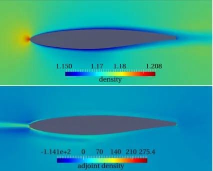
For the time and memory measurements, we run mgopt on a test case simulating external flow around a truncated RAE2822 airfoil, see Figure 1. The domain is discretised with 23458 mesh nodes. We use a 2nd order Roe flux, with an explicit solver scheme for the inner iterations. The Spalart-Almaras turbulence model is used and fully differentiated. We use a fixed number of 300 inner iterations as a stopping criterion for both primal and adjoint solvers for the time
mea-density 1.17 1.18 1.208 1.150 adjoint density 0 70 140 210 -1.141e+2 275.4
Fig. 1: Primal and adjoint density field on a truncated RAE2822 airfoil. The adjoint flow (bot-tom) shows a wake going in the opposite flow direction, the leading edge is highly sensitive as expected.
surement, with 1 physical time step. The flow was set up with a freestream Mach number of Ma∞= 0.2 at an angle of attack of 0◦. The cost function for the adjoint field was drag.
To simplify the discussion that follows, we assume that all differentiated procedures are dom-inated by a single procedure called residual(R ↓, X ↑,U ↑) that is the only differentiation head passed to Tapenade. The residual result R forms the basis for the update of the flow state U either by an explicit step or after a linear solver call. The geometry of the problem (node coordinates, surface normals, cell volumes etc.) are denoted by X . Arrows pointing upward mark procedure outputs, whereas downward arrows mark procedure inputs.
We compare two setups. The first, referred to as specialised setup, uses two differentiation heads for the residual procedure, resulting in the two differentiated procedures residual_b_x(R ↓ , ¯R ↑, X ↑, ¯X ↓,U ↑, ¯U ↓) and residual_b_u(R ↓, ¯R ↑, X ↑,U ↑, ¯U ↓). They are used in the adjoint solver
as shown in Algorithm 1, making use of the fact that the primal flow solver is a nonlinear fixed-point loop, for which [Christianson 1994] presented a proof that adjoint gradients can be com-puted without storing intermediate stages of the primal loop. Our implementation resembles the recipe presented in [Giering and Kaminski 1998] that uses the reverse-differentiation of the primal procedure in the adjoint loop. We observe that the derivatives with respect to X are not evolved in the adjoint loop and use multi-activity differentiation to remove the computation of
¯
X . In addition, we use thespecializeActivity %all%command line flag to create specialised procedures wherever possible.
The second, referred to as the generalised setup, does not make use of the new multi-activity AD. We use one differentiation head for the residual procedure, yielding residual_b(R ↓, ¯R ↑, X ↑
, ¯X ↓,Ut↑, ¯Ut↓). This is used instead of residual_b_x and residual_b_u throughout the code. We do not use command line flags or pragmas for multi-activity AD in this setup.
Let us first consider the time it takes for Tapenade to complete the differentiation of the code, and the size of the resulting derivative code:
ALGORITHM 1: mgopt primal and adjoint flow solver Input: Initial guess U0, design vector X
Output: Flow field trajectory U1. . .Utfinal, cost J , sensitivity of cost wrt. design ¯X
t ← 0
while t < tfinaldo// unsteady primal loop
Ut +1← Ut// initial guess from previous forward step
t ← t + 1
repeat
foreach RK stage, MG cycle do
residual(R ↓, X ↑,Ut↑)// primal residual() update(Utl, R ↑)
MG_and_RK_transfer() end
until kRk ≤ cutoff end
if primal only then cost(J ↓,Ut↑, X ↑) else
¯
J ← 0
cost_b(J ↓, ¯J ↑,Ut↑, ¯Ut↓, X ↑, ¯X ↓)
while t ≥ 0 do// unsteady adjoint loop repeat
foreach RK stage, MG cycle do
MG_and_RK_transfer_adj()// recycled MG_and_RK_transfer() update_adj(Utl, ¯Utl, R ↑, ¯R ↓)// hand-coded adjoint of update()
residual_b_u(R ↓, ¯R ↑, X ↑,Ut↑, ¯Ut↓)// generated by Tapenade from residual() end
until R ≤ cutoff
Vt −1← Vt// initial guess for next reverse step
t ← t − 1
end
residual_b_x(R ↓, ¯R ↑, X ↑, ¯X ↓,Ut↑, ¯Ut↓)// generated by Tapenade from residual() end
diff time diff code lines diff code chars executable size
general 6.270s 22122 880514 1.8MB
special 8.394s 34728 1350785 2.2MB
change 34% 57% 53% 22%
The specialisation results in an increase in code size of more than 50%, which manifests itself in a slightly larger executable file. The relative increase is smaller for the binary file, since it includes also non-differentiated procedures and statically linked libraries. The runtime of Tapenade only increases by a third, which is less than the linear worst-case complexity with respect to output code size predicted in Sec. 4.
Next, we consider the total runtime measured with gprof and peak memory usage measured by reading the reported high water mark from/proc/PID/statusfor the airfoil case on a system running Scientific Linux 6.2 on a Intel Xeon E5-2660 CPU.
total runtime relative time residual runtime relative time peak
memory memoryrelative
primal 51.15s 1 38.71 1 360.93MB 1
general 247.14s 4.83 239.56 6.2 431.68MB 1.196
special 186.5s 3.65 177.51 4.6 432.62MB 1.199
change -25% -26% 0.2%
The adjoint solver runs about a quarter faster in the specialised setup than in the generalised setup. There is no considerable change in the memory usage (half of the difference is caused by the size of the executable itself ). It is also worth considering the relative runtime compared to the primal solver. In the specialised setup, the adjoint solver takes 4.6 times longer per iteration, the general solver needs more than 6 times longer than the primal solver per iteration.
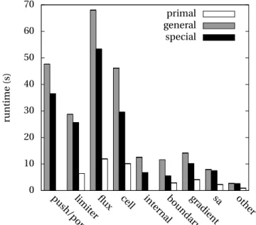
To understand how multi-activity AD resulted in the observed speedups, we identify main functionalities that are dominated by the differentiation head for which we measure the timings separately. To give an example: The turbulence model consists of a main procedure that calls several helper procedures. The time spent in all these is summed up and referred to under the name turbulence. Other functionalities that we time separately are internal, boundary, residual,
gradient, limiter and cell correction. We only consider the self time of all these functionalities, i.e.
time spent inside the flux calculation is already encountered for inside flux and therefore does not contribute to the timing of internal or boundary, from which flux is called. The call graph that we obtain by clustering all utility procedures together into these core functionalities is shown in Figure 2, along with the call graph of the clustered adjoint code obtained in the specialised setup. The specialised setup has a lower runtime for all functionalities, as shown in detail in Fig-ure 3. Taken together, the primal and adjoint residual and all procedFig-ures dominated by them contribute 177s to the runtime in specialised mode and 240s in generalised mode. About 10s are spent in other procedures such as libraries and linear solvers.
We see a significant overall reduction of time spent on the Tapenade push/pop stack mecha-nism. Furthermore, we can observe three possible outcomes of applying multi-activity AD: 6.1. No speedup
For the cell gradient, Tapenade creates specialisations caused by call sites inside a branch specif-ically for the temperature gradient computation. In this branch, the temperature field is stored inside a temporary variable that is overwritten after calling the gradient computation, making the temperature varied, but not useful. At other call sites, the field for which the gradient is com-puted is active. Without specialisation, the differentiation is performed assuming that the tem-perature t is a useful differentiation result, requiring the creation and initialisation of a dummy t in the calling context that is never used. In specialisation mode, the differentiation uses the cor-rect activity, i.e. t is not initialised by the calling context. However, it has to be initialised inside the differentiated procedure instead, removing any performance benefit, see Algorithm 2. ALGORITHM 2: Comparison of gradient calculation with generalised and specialised activity. In this case, multi-activity AD did not reduce the number of instructions at all.
Proceduregradient_b_general(∇U , ∇U)
t ← ∇U t ← 0
callcellGradient_b_general(t emp, t) ∇U ← ∇U + t return ProcedurecellGradient_b_general(t , t) ...forward sweep ...backward sweep return
Proceduregradient_b_special(∇U , ∇U)
t ← ∇U callcellGradient_b_special(t , t) ∇U ← ∇U + t return ProcedurecellGradient_b_special(t , t) ...forward sweep t ← 0 ...backward sweep return
6.2. Reverse computation speedup
The speedup ratio achieved by specialisation is most pronounced for the boundary treatment. The runtime for the specialised code was measured as 5750ms, while the generalised code runs for 10890ms, about 2 times longer. This runtime difference is caused by a procedure within the boundary treatment that at every boundary node projects the local gradient vector ∇U into the local surface normal direction n by computing (∇U · n) · n, which is a non-linear dependency of the output with respect to the input n. If n is active, this requires that intermediate variables during the iteration over boundary nodes are stored in the forward sweep and loaded in the backward sweep. If n is inactive, there is no nonlinear influence in this procedure and the forward sweep is not needed at all. See Algorithm 3 for an example where Tapenade removed calls to the storing mechanism in addition to some computations, or Appendix B for a more detailed example in Fortran.
ALGORITHM 3: Differentiated symmetry gradient correction. The primal procedure subtracts the boundary-surface normal component of the gradient. The gradient values are not needed for the differ-entiated procedure if only the gradient itself is active, as it is the case for the procedures dominated by residual_b_u. This allows Tapenade to remove all statements highlighted in grey.
ProceduresymmetryPlane(∇U , n)
t ← 0
while i <numberOfBoundaryNodes do
k ←lookupVolumeIdFromBoundaryId(i )
∇Uk← ∇Uk−¡∇Uk· ni¢ · ni
i ← i + 1
end return
ProceduresymmetryPlane_b(∇U , ∇U , n , n)
t ← 0
while i <numberOfBoundaryNodes do
k ←lookupVolumeIdFromBoundaryId(i )
∇Uk← ∇Uk−¡∇Uk· ni¢ · ni
pushToStack(∇Uk) i ← i + 1 end while i ≥ 0 do i ← i − 1 k ←lookupVolumeIdFromBoundaryId(i ) ∇Uk←popFromStack() n ← n −¡∇Uk· n¢ · ∇Uk ∇Uk← ∇Uk+ ³ ∇Uk· ni ´ · ni n ← n +³∇Uk· n ´ · ∇Uk end return
6.3. Forward computation speedup
In the cell gradient correction computation, some intermediate results only need to be com-puted if geometry variables are active, which is not the case for procedures dominated by residual_b_u, and so the diff-liveness analysis discards some statements and procedure calls in the forward computation of the adjoint solver. An example for this is given in Appendix A.
residual_b_u residual_b_x boundary internal gradient turbulence flux limiter cell correction b0 b b0 b b b0 b1 b b1 b2 b0 b2 b0 b b b0 b3 b2 b b1 b0 residual boundary internal gradient turbulence flux limiter cell correction
Fig. 2: Primal (bottom left) and differentiated call graphs (top right). Each arrow in the differen-tiated call graph represents a specialised differendifferen-tiated procedure that is named with the suffix indicated on the arrow. We can identify two main streams: Code dominated byresidual_b_u
(lines) andresidual_b_x(dashes).
0 10 20 30 40 50 60 70 runt ime (s) primal general special oth er sa gr adien t boundar y int er na l cell flux lim iter push /pop
7. CONCLUSION, FUTURE WORK
We developed a refined static activity analysis that, based on a context-sensitive analysis and user input, employs procedure cloning and specialisation to generate more efficient derivative code in source-transformation algorithmic differentiation (AD). The method was implemented in the AD tool Tapenade. A case study shows that our approach can provide substantial benefits in the adjoint runtime, at virtually no cost in memory footprint. The cost in terms of derivative code size and differentiation time is significant, but typically less important than the perfor-mance gains in the generated derivative code.
The refined activity analysis improves code performance drastically in some circumstances, but produces unnecessary derivative code in some cases. A user could intervene manually using command line options and pragmas to avoid this. In the future, this could be addressed with a more sophisticated specialisation strategy that only creates specialised procedures where a benefit can be expected.
If the generalisation mode is used, there can be cases with more than one possible way to link differentiated procedures to call sites. The current behaviour of Tapenade is implementation-defined and arbitrary. This could be improved to choose the most cost-effective specialisation.
Another possible extension could be made for branches and other control flow statements. The specialisation for procedures was possible because each procedure can be accessed from multiple call sites with different activities. Likewise, a code portion after an if/else block could be reached with different activities depending on the branch chosen in the preceding block. The same holds true for code that can be reached through return, cycle, goto or similar statements. Specialisation could be used in these cases.
APPENDIX
ACKNOWLEDGMENTS
This work has been conducted within the About Flow project on “Adjoint-based optimisation of industrial and unsteady flows”. The project has received funding from the European Union’s Seventh Framework Programme for research, tech-nological development, and demonstration under grant agreement no 317006.
This research utilised Queen Mary University of London’s MidPlus computational facilities, supported by QMUL Research-IT and funded by EPSRC grant EP/K000128/1.
REFERENCES
Christian Bischof, Alan Carle, George Corliss, Andreas Griewank, and Paul Hovland. 1992. ADIFOR–generating derivative codes from Fortran programs. Scientific Programming 1, 1 (1992), 11–29.
Martin Bücker, Bruno Lang, Arno Rasch, Christian H. Bischof, and Dieter an Mey. 2002. Explicit loop scheduling in OpenMP for parallel automatic differentiation, In Annual International Symposium on High Performance Com-puting Systems and Applications. High Performance ComCom-puting Systems and Applications, 2002. Proceedings. 16th
Annual International Symposium on 16 (2002), 121–126.DOI:http://dx.doi.org/10.1109/HPCSA.2002.1019144
Faidon Christakopoulos, Dominic Jones, and Jens-Dominik Müller. 2011. Pseudo-timestepping and veri-fication for automatic differentiation derived CFD codes. Computers Fluids 46, 1 (2011), 174 – 179. DOI:http://dx.doi.org/10.1016/j.compfluid.2011.01.039
Bruce Christianson. 1994. Reverse accumulation and attractive fixed points. Optimization Methods and Software 3, 4 (1994), 311–326.
Mike Fagan and Alan Carle. 2004. Activity analysis in ADIFOR: Algorithms and effectiveness. Technical Report. Technical Report TR04-21, Department of Computational and Applied Mathematics, Rice University, Houston, TX.
Ralf Giering. 1999. Tangent linear and Adjoint Model Compiler , Users manual 1.4.
Ralf Giering and Thomas Kaminski. 1998. Recipes for adjoint code construction. ACM Transactions on Mathematical
Software (TOMS) 24, 4 (1998), 437–474.
Ralf Giering, Thomas Kaminski, Ricardo Todling, Ronald Errico, Ronald Gelaro, and Nathan Winslow. 2006. Tangent linear and adjoint versions of NASA/GMAO’s Fortran 90 global weather forecast model. In Automatic Differentiation:
Applications, Theory, and Implementations. Springer, 275–284.
Michael B. Giles. 2000. On the use of Runge-Kutta time-marching and multigrid for the solution of steady adjoint
Andreas Griewank and Andrea Walther. 2000. Algorithm 799: Revolve: An Implementation of Checkpointing for the Reverse or Adjoint Mode of Computational Differentiation. ACM Trans. Math. Softw. 26, 1 (March 2000), 19–45. DOI:http://dx.doi.org/10.1145/347837.347846
Laurent Hascoët, Stefka Fidanova, and Christophe Held. 2002. Adjoining Independent Computations. In
Au-tomatic Differentiation of Algorithms, from Simulation to Optimization. Springer New York, 299–304. DOI:http://dx.doi.org/10.1007/978-1-4613-0075-5{_}35
Laurent Hascoët and Valérie Pascual. 2012. The Tapenade Automatic Differentiation tool: principles, model, and
specifi-cation. INRIA Research Report RR-7957. 53 pages.
Laurent Hascoet and Valérie Pascual. 2013. The Tapenade Automatic Differentiation Tool: Princi-ples, Model, and Specification. ACM Trans. Math. Softw. 39, 3, Article 20 (May 2013), 43 pages. DOI:http://dx.doi.org/10.1145/2450153.2450158
Gilles Kahn. 1987. Natural semantics. Springer.
Barbara Kreaseck, Luis Ramos, Scott Easterday, Michelle Strout, and Paul Hovland. 2006. Hybrid static/dynamic activity analysis. In Computational Science–ICCS 2006. Springer, 582–590.
J-D Müller and P Cusdin. 2005. On the performance of discrete adjoint CFD codes using automatic differentiation.
Inter-national journal for numerical methods in fluids 47, 8-9 (2005), 939–945.
Uwe Naumann. 2004. Optimal Accumulation of Jacobian Matrices by Elimination Methods on the Dual Computational Graph. Math. Program. 99, 3 (April 2004), 399–421.DOI:http://dx.doi.org/10.1007/s10107-003-0456-9
Jaewook Shin and Paul D. Hovland. 2007. Comparison of Two Activity Analyses for Automatic Differentiation: Context-sensitive Flow-inContext-sensitive vs. Context-inContext-sensitive Flow-Context-sensitive. In Proceedings of the 2007 ACM Symposium on
Ap-plied Computing (SAC ’07). ACM, New York, NY, USA, 1323–1329.DOI:http://dx.doi.org/10.1145/1244002.1244287
Jaewook Shin, Priyadarshini Malusare, and Paul D. Hovland. 2007. Design and Implementation of a Context-Sensitive, Flow-Sensitive Activity Analysis Algorithm for Automatic Differentiation. In 5th International Conference on
Auto-matic Differentiation (AD 2008), Vol. 64. Lect. Notes Comput. Sci. Eng., Lect. Notes Comput. Sci. Eng., Bonn,
Ger-many, 115–125.
Jean Utke, Uwe Naumann, Mike Fagan, Nathan Tallent, Michelle Strout, Patrick Heimbach, Chris Hill, and Carl Wunsch. 2008. OpenAD/F: A Modular Open-Source Tool for Automatic Differentiation of Fortran Codes. ACM Trans. Math.
Softw. 34, 4, Article 18 (July 2008), 36 pages.DOI:http://dx.doi.org/10.1145/1377596.1377598
Qiqi Wang, Parviz Moin, and Gianluca Iaccarino. 2009. Minimal Repetition Dynamic Checkpointing Algorithm for Unsteady Adjoint Calculation. SIAM Journal on Scientific Computing 31, 4 (2015/05/03 2009), 2549–2567. DOI:http://dx.doi.org/10.1137/080727890
Shenren Xu, David Radford, Marcus Meyer, and Jens-Dominik Müller. 2015. Stabilisation of discrete steady adjoint solvers. J. Comput. Phys. 299 (2015), 175–195.
Received August 2015; revised January 2099; accepted June 2099
A. CODE EXAMPLE FOR SPEEDUP OF FORWARD COMPUTATION
This illustrates why there is less time spent in primal procedures during the cell gradient calculation if specialisation is used. In the specialisation used in procedures dominated by residual_b_u, the element volume is not active. In contrast, specialisations where the volume is active require that the gradient is calculated so thatvolumesumbcan be updated, contributing to the time spent in primal procedures.
1 s u b r o u t i n e c e l l G r a d ( U , gradU , v o l u m e S u m ) 2 r e a l gradU , U , v o l u m e S u m 3 4 c a l l c a l c G r a d ( U , g r a d U ) ! r e t u r n s g r a d * vol 5 g r a d U = g r a d U / v o l u m e S u m ! n o r m a l i s e 6 end s u b r o u t i n e 1 ! a c t i v e v a r i a b l e s : u g r a d u v o l u m e s u m 2 C A L L C A L C G R A D ( u , g r a d u ) 3 v o l u m e s u m b = v o l u m e s u m b - g r a d u * g r a d u b / v o l u m e s u m **2 4 g r a d u b = g r a d u b / v o l u m e s u m 5 C A L L C A L C G R A D _ B ( u , ub , gradu , g r a d u b )
6 g r a d u b = 0.0
1 ! a c t i v e v a r i a b l e s : u g r a d u 2 g r a d u b = g r a d u b / v o l u m e s u m
3 C A L L C A L C G R A D _ B ( u , ub , gradu , g r a d u b )
4 g r a d u b = 0.0
B. CODE EXAMPLE FOR SPEEDUP OF REVERSE COMPUTATION
Symmetry correction primal code and body of specialised differentiated codes. Note that the backward sweep has around twice as many instructions in this example ifnrmis active, leading to the difference in adjoint runtime. In addition, there are calls to the data stack, which leads to an increased time spent on the push/pop stack.
1 s u b r o u t i n e s y m m e t r y C o n d ( n B n d N o d e , nNode , gradU , nrm , idx )
2 i n t e g e r n N o d e ! n u m b e r of m e s h n o d e s ( v o l u m e + b o u n d a r y )
3 i n t e g e r n B n d N o d e ! n u m b e r of b o u n d a r y n o d e s
4 i n t e g e r idx ( n B n d N o d e ) ! ID of b o u n d a r y n o d e s in m e s h no d e a r r a y
5 r e a l nrm ( n B n d N o d e ,3) ! s u r f a c e n o r m a l s for b o u n d a r y n o d e s
6 r e a l g r a d U ( nNode ,3) ! g r a d i e n t ( U ) for all m e s h n o d e s
7 i n t e g e r i
8
9 do i =1 , n B n d N o d e
10 g r a d U ( idx ( i ) ,:) = g r a d U ( idx ( i ) ,:) &
11 & - sum ( g r a d U ( idx ( i ) ,:)* nrm ( i , : ) ) * nrm ( idx ( i ) ,:)
12 end do
13 end s u b r o u t i n e
1 ! a c t i v e v a r i a b l e s : g r a d U 2 DO i =1 , n b n d n o d e
3 r e s u l t 1 = SUM ( g r a d u ( idx ( i ) , :)* nrm ( i , :))
4 g r a d u ( idx ( i ) , :) = g r a d u ( idx ( i ) , :) - r e s u l t 1 * nrm ( idx ( i ) , :)
5 END DO
6 DO i = n b n d no d e ,1 , -1
7 r e s u l t 1 b = - SUM ( nrm ( idx ( i ) , :)* g r a d u b ( idx ( i ) , :))
8 g r a d u b ( idx ( i ) , :) = g r a d u b ( idx ( i ) , :) + nrm ( i , :)* r e s u l t 1 b 9 END DO 1 ! a c t i v e v a r i a b l e s : gradU , nrm 2 DO i =1 , n b n d n o d e 3 C A L L P U S H R E A L 4 ( r e s u l t 1 ) 4 r e s u l t 1 = SUM ( g r a d u ( idx ( i ) , :)* nrm ( i , :)) 5 C A L L P U S H R E A L 4 A R R A Y ( g r a d u ( idx ( i ) , :) , 3)
6 g r a d u ( idx ( i ) , :) = g r a d u ( idx ( i ) , :) - r e s u l t 1 * nrm ( idx ( i ) , :)
7 END DO
8 DO i = n b n d no d e ,1 , -1
9 C A L L P O P R E A L 4 A R R A Y ( g r a d u ( idx ( i ) , :) , 3)
10 r e s u l t 1 b = - SUM ( nrm ( idx ( i ) , :)* g r a d u b ( idx ( i ) , :))
11 n r m b ( idx ( i ) , :) = n r m b ( idx ( i ) , :) - r e s u l t 1 * g r a d u b ( idx ( i ) , :)
12 C A L L P O P R E A L 4 ( r e s u l t 1 )
13 g r a d u b ( idx ( i ) , :) = g r a d u b ( idx ( i ) , :) + nrm ( i , :)* r e s u l t 1 b 14 n r m b ( i , :) = n r m b ( i , :) + g r a d u ( idx ( i ) , :)* r e s u l t 1 b