Articulated pose estimation via over-parametrization and noise projection

(1)

Articulated Pose Estimation via

Over-parametrization and Noise Projection

by MAS

Jonathan David Brookshire

B.S., University of Virginia (2002) M.S., Carnegie Mellon University (2004)

gACHN

SACHUSETTf-1S IEffU

OF TECHNOLOGY

APR

10 2014

LIBRARIES

Submitted to the Department of Electrical Engineering and Computer Science

in partial fulfillment of the requirements for the degree of Doctor of Philosophy

at the

MASSACHUSETTS INSTITUTE OF TECHNOLOGY February 2014

@

Author ... . ...

Department of Electrical E 'neeri and Computer Science September 30, 2013 Certified by ... ... Seth Teller Professor Thesis Supervisor Accepted by .... Lesa

i.

Kolodziejski

(2)

Articulated Pose Estimation via Over-parametrization and Noise Projection

by

Jonathan David Brookshire

Submitted to the Department of Electrical Engineering and Computer Science on September 30, 2013, in partial fulfillment of the requirements for the degree of

Doctor of Philosophy

Abstract

Outside the factory, robots will often encounter mechanical systems with which they need to interact. The robot may need to open and unload a kitchen dishwasher or move around heavy construction equipment. Many of the mechanical systems encoun-tered can be described as a series of rigid segments connected by joints. The pose of a segment places constraints on adjacent segments because they are mechanically 'connected. When modeling or perceiving the motion of such an articulated system, it is beneficial to make use of these constraints to reduce uncertainty. In this thesis, we examine two aspects of perception related to articulated structures. First, we ex-amine the special case of a single segment and recover the rigid body transformation between two sensors mounted on it. Second, we consider the task of tracking the configuration of a multi-segment structure, given some knowledge of its kinematics.

First, we develop an algorithm to recover the rigid body transformation, or ex-trinsic calibration, between two sensors on a link of a mobile robot. The single link, a degenerate articulated object, is often encountered in practice. The algorithm re-quires only a set of sensor observations made as the robot moves along a suitable path. Over-parametrization of poses avoids degeneracies and the corresponding Lie algebra enables noise projection to and from the over-parametrized space. We demon-strate and validate the end-to-end calibration procedure, achieving Cramer-Rao Lower Bounds. The parameters are accurate to millimeters and milliradians in the case of planar LIDARs data and about 1 cm and 1 degree for 6-DOF RGB-D cameras.

Second, we develop a particle filter to track an articulated object. Unlike most previous work, the algorithm accepts a kinematic description as input and is not specific to a particular object. A potentially incomplete series of observations of the object's links are used to form an on-line estimate of the object's configuration (i.e., the pose of one link and the joint positions). The particle filter does not require a reliable state transition model, since observations are incorporated during particle proposal. Noise is modeled in the observation space, an over-parametrization of the state space, reducing the dependency on the kinematic description. We compare our method to several alternative implementations and demonstrate lower tracking error for fixed observation noise.

Thesis Supervisor: Seth Teller Title: Professor

(3)

Acknowledgments

This work would not have been possible without the support of many people. I would first thank my advisor, Professor Seth Teller. Seth repeatedly astounded me with his breadth of knowledge and ability to quickly reach conclusions I gleaned only after a period of long reflection. He provided that delicate balance of guidance: enough to be helpful, but not so much as to be obtrusive. For their sake, I hope he continues to mentor students for many years to come.

Thanks also to my committee members, Professors Tomis Lozano-Perez and Berthold Horn. They have contributed greatly to this work. I have appreciated their insightful comments and feedback.

My lab mates in the RVSN group were also crucial to this thesis. Much thanks to Albert Huang and Luke Fletcher for helping me get rolling with the forklift in the early days. Matt Walter and Matt Antone were both tremendously helpful and kind individuals: their intelligence was matched only by their humility. Steve Proulx was an invaluable teammate and helped keep the equipment operational and provide a sanity check on ideas. Thanks also to Bryt Bradley for having everything organized making all of our work possible. It has been a great pleasure to work with Mike Fleder, Sudeep Pillai, and Sachi Hemachandra over the past few years.

To give the proper thanks to my family would take more than the remainder of this document. My mom and dad have provided constant support throughout my life. My wife has been a constant source of strength and patience and reminded me about life outside these pages. My new daughter has provided motivation and focus.

(4)

List of Figures

1-1 The sensors on a robotic platform (left) form a simple, rigid mechanical

chain. The arm of a backhoe (right) forms a more complex mechanical chain with several joints. . . . . 15

2-1 Both these autonomous vehicles require extrinsic sensor calibration to fuse data from multiple sensors. . . . . 19 2-2 As the robot moves from pi to p₃, two sensors (positioned as in (a))

will experience different translational ((b) and (c)) and rotational (not shown) incremental motion. The calibration relating the sensors is the transformation that best brings the disparate observed motions into agreem ent. . . . . 20 2-3 Calibration solutions requiring SLAM attempt to establish a common

reference frame for the sensors (blue and red) using landmarks (green). 26 2-4 Graphical model of calibration and incremental poses is shown . . . . 29 2-5 Incremental poses for the r (red) and s (blue) sensors are observed as

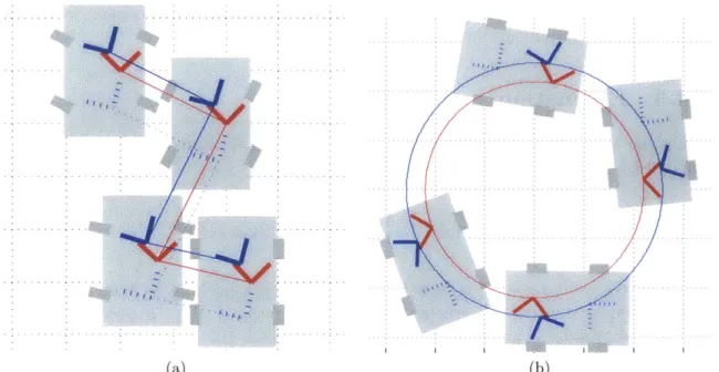
the robot travels. The observations are plotted on the right in x-y-O coordinates. The true calibration parameters will transform the red and blue observations into alignment. . . . . 29 2-6 Sensor movements without rotation, as for a translating holonomic

robot (which can move in any dimension regardless of state) (a), can prevent calibration. (The dotted blue lines show blue sensor poses corresponding to alternative calibration parameters.) The calibration of a non-holonomic robot (e.g., an automobile) cannot be recovered if the robot is driven in a straight line. Concentric, circular sensor motion (b) can also prevent calibration. . . . . 33 2-7 Resampling incremental poses (blue) at new time steps may make

in-terpolated observations (black) dependent. . . . . 36 2-8 A robot travels along a mean path (blue) starting from the bottom

and ending in the upper left. Gray lines show the sigma points, Xi, each representing a path. Points associated with each sample time are shown as block dots. . . . . 39 2-9 The sigma points are resampled to produce the Yi paths (gray lines)

(8)

2-10 The original mean path (blue) at times A and resampled mean path

(red) at tim es B . . . . 40

2-11 Observations drawn from each paused interval can be compared to

estimate incremental pose covariances off-line. . . . . 43

2-12 A simulated travel path for sensor r (blue), with calibration k =

[-0.3 m, -0.4 m, 300] applied to sensor s (red). Two example sensor

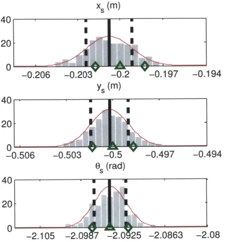
frames are shown at pi and P2. . . . . 43 2-13 Histograms (gray) of calibration estimates from 200 simulations of the

path in Figure 2-12 match well with truth (triangles) and the CRLB (diamonds). Vertical lines indicate mean (solid) and one standard

de-viation (dashed). . . . . 44

2-14 For 30 different simulated calibration runs, the parameter standard de-viation (left, green) and CRLB (left, yellow) match well. Additionally,

the Box bias is relatively small compared to the CRLB. . . . . 45

2-15 The CRLB increases with observation noise. . . . . 46

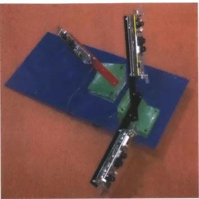
2-16 The robot test platform with configurable hardware, provides ground

truth calibrations. . . . . 47

2-17 Paths of r and s when k = [-0.2m, -0.5m, -120'] are shown. ... 47

2-18 Estimates from 200 trials using real path of Figure 2-17 are shown. 48

2-19 We recovered the closed calibration chain between the two LIDARs

{r,

s} and the robot frame (u, combined IMU and odometry). .... 49

2-20 The incremental motions of the r (red) and s (blue) sensors are used

to recover the calibration between the sensors as the robot moves. The dotted lines suggest the incremental motions, vri and vsi, for sensors r

and s, respectively. . . . . 50

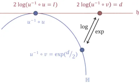
2-21 The mapping between the Lie group, H, and the Lie algebra, j, is

performed at the identity, i.e., u-1 o u. . . . . 53

2-22 Three different methods for interpolating between the cyan and ma-genta poses are depicted. The DQ SLERP is used in (a), the quaternion SLERP is used in (b), and a linear interpolation in Euler angles is used

in (c). The right column shows the linear and angular velocities. . . . 57

2-23 Visualization of the matrix JGU shows that only the first six columns

can be reduced. Blank entries are zero, orange are unity, and red are

more complex quantities. . . . . 62

2-24 Two robots driven along the suggested paths experience rotation about only one axis (green). As a result, the true calibration relating the two true sensor frames (red/blue) cannot be determined. The magenta

(9)

2-25 Motion is simulated such that the red and blue sensors traveled the paths as shown. (The path is always non-degenerate.) In this image

k = [0., 0.05, 0.01 0, 0, ]... . . . ... 67

2-26 _{Histograms (gray) of calibration estimates from 400 simulations of the}

path in Figure 2-25 match well with the true calibration (green trian-gles) and constrained CRLB (green diamonds). Black lines indicate the sample mean (solid) and one standard deviation (dashed); the red lines show a fitted Gaussian. . . . . 69 2-27 The error between the known calibration and the mean estimate was

less than ±0.01 for each DQ parameter. Parameter qo-q4 are shown here. 70

2-28 The error between the known calibration and the mean estimate was less than ±0.01 for each DQ parameter. Parameter q5-q7 are shown here. 71

2-29 We assess the method's consistency by recovering the loop of calibra-tions relating three RGB-D sensors. . . . . 72 3-1 In this motivating construction site example, the two excavators must

be tracked and avoided by an autonomous system. Yellow lines shows a notional kinematic chain provided as input to our tracking system. . 74 3-2 A robot non-rigidly gripping a pipe and a dishwasher with a door and

shelves are examples of articulated systems we consider . . . . 76 3-3 A stream of observations and a static kinematic model are inputs to

the Articulated Object Tracker. The tracker estimates the object's base pose and joint values (i.e., the object's configuration). . . . . 76 3-4 The goal of the articulated object tracker is to estimate the joint values

and base pose of an articulated object, such as the excavator shown here. Observations might be image detections. . . . . 77 3-5 The current observation, Zk (black dotted line), intersects the possible

configurations (red line) at four places which indicates four possible configurations that explain the observation. For each cycle of the par-ticle filter algorithm, the previous generation of parpar-ticles (a) is used to sample from a proposal distribution (M is f(x), the observation manifold). In (a), particles are represented by their position along the x-axis; their weight is their height. Particles are colored consistently from (a)-(d). Here, the state transition model P(XlXk-1) is used to predict the particle evolution (b). The weights are updated via the observation density, P(zlx), in (c) and the next generation of particles result (d). Resampling (not shown) may then be necessary. . . . . 87 3-6 Each row shows a sample scenario from different views (columns). The

gray rendering is the true pose, shown alone in the first column and in the background in other columns. The magenta renderings show alternative configurations which also explain the observations (rays). In all these examples, multiple modes explain the observations. .... 96

(10)

3-7 In situations where the observation model is more accurate than the

state transition model, many samples must be drawn from P(Xklzk-1)

to capture the peak of P(zk Xk). . . . . 97

3-8 An example planar articulated system with four rigid links and three

revolute joints. . . . . 97

3-9 The dots show the link positions of the particles proposed from P(Xk XI 1)

for links 1-4 (respectively blue, red, green, and magenta). The

under-lying contours (black) illustrate the Gaussian P (ZkIXk). Notice that

for link 4, for example, many particles are unlikely according to the observation model. An example configuration for the linkage is also

show n . . . . 99

3-10 In the baseline method, altering the state parametrization also affects

the proposed particles (c.f., Figure 3-9) . . . . 99

3-11 Different state parametrizations result in different sigma points for the UKF (a), (b). The sigma points for links 1-4 are shown here in blue,

green, red, and cyan, respectively. In this situation, different tracking

error (c) results. Error bars indicate one standard deviation. . . . . . 101

3-12 The method updates the previous particle, xi, with the observations,

Zk, using the Taylor approximation and subsequent projection. .... 105

3-13 A Taylor approximation and a projection relate noise in observation

space to noise in state space. . . . . 105

3-14 Proposing particles at singularities . . . . 108

3-15 An observation (dotted line) is obtained in (a); intersections with M

(red) are likely configurations (black squares). The particles (Xk_1)

are then optimized (b) toward the likely configurations (Mk, color

as-terisks). Random perturbations are added in the observation space (c). For each particle, XW in (d) approximates the QIF. XW is then

sampled to select the next generation of particles (e). . . . . 110

3-16 Examples of singular observations along rays associated with image

observations are shown. . . . . 113

3-17 Qualitative comparison of optimization, UKF, baseline PF, and our

method. Red indicates not supported; yellow indicates supported

un-der additional conditions; and green, indicates fully supported. . . . 117

3-18 The Naive method of calculating the pseudo-inverse (dashed line)

suf-fers from a singularity when an eigenvalue is zero, i.e., - = 0. Several

heuristics exist for handling this situation in practice. . . . . 120

3-19 Results for the kinematic chain. Error bars show one standard

devia-tion about the m ean. . . . . 121

3-20 Different state parametrizations do not significantly affect the RMSE

for the four-link kinematic chain. The error bars indicate one standard

(11)

3-21 The dishwasher consists of two articulated drawers and one door. Joint limits prevent configurations in which the door and drawers would overlap or extend beyond physical limits. Yupper and ylower are static parts of the kinematic model. . . . . 122 3-22 Results for the dishwasher simulation are shown. . . . . 123 3-23 The true motion of a 4-link chain (blue) is shown in the middle column

for several sample frames. Observations are shown as black squares. For each frame (row), the configurations associated with the particles are shown on the right (black). Note that until frame 24, when the motion of the chain is unambiguous, two clusters are maintained by the particles. . . . . 124 3-24 Particle weights are divided between two clusters explaining the

ob-servations until the system moves to disambiguate the configuration. With noise-free observations, the weights would be nearly equal until frame 24; the results from noisy observations shown here cause the particle weights to deviate from exactly 50%. . . . . 125 3-25 Sigma points for UKF simulations. . . . . 126 3-26 The same parametrization is used for two different simulations,

result-ing in different UKF performance, relative to our method (see Fig-ure 3-27). . . . . 127 3-27 The RMSE performance of our method and the UKF is similar for

Simulation #1, where the parametrization produces favorable sigma points. This is not always the case, however, as illustrated by Simu-lation #2. The x-axis location of the UKF results corresponds to the number of sigma points. . . . . 128 3-28 Sample configurations for this 5-DOF toy example were constructed

with "stop-frame" style animation. . . . . 128 3-29 For the kinematic chain, proposing noise in the observation space

(green) yields RMSE improvement over the baseline approach (blue). RMSE is further reduced (red) by centering proposals around the ob-servations. . . . . 129 3-30 A TLD tracker provided positions of the dishwasher's articulated links

as input. A vertical was also extracted. . . . . 130 3-31 In addition to lower RMSE, our method demonstrated less variation in

accuracy while tracking the dishwasher, because it quickly recovered when missing observations resumed. . . . . 130 3-32 The baseline and our method are affected similarly by model noise.

Dotted lines show one standard deviation. . . . . 131 3-33 The PR2's grip on the pipe is not rigid, but still constrains some

(12)

3-34 In this sequence, the PR2 rotates the pipe. (a) shows the pipe poses color coded by time; the pipe proceeds through red-yellow-blue poses. The two large velocity spikes in (b) correspond to times when the pipe

underwent significant slip in the gripper. . . . . 133

3-35 In this sequence, the PR2 moved its gripper so as to rotate the pipe

approximately along its long axis (here, nearly vertical). . . . . 133

3-36 RMSE and number of effective particle performance for the pipe-swing

sequence in Figure 3-34 are shown. . . . . 134

3-37 RMSE and number of effective particle performance for the axis-rotate

sequence in Figure 3-35 are shown. . . . . 134

3-38 At HCA in Brentwood, NH, operators train on several different types

of equipment in parallel. . . . . 135

3-39 We captured operation of an excavator with a PointGrey camera (mounted

left) and 3D LIDAR (mounted right). . . . . 136

3-40 The CATERPILLAR 322BL excavator was modeled in SolidWorks

us-ing specifications available online [62]. . . . . 136

3-41 The excavator loads a dump truck three times. Viewed from above, this graphic shows the entire 1645-frame sequence, color coded by time.

The three loads correspond to blue, yellow, and red, in that order. . . 137

3-42 These plots show errors, failures, and number of effective particles for the excavator example. The top row shows the sample RMSE plot at

different zoom scales. . . . . 139

3-43 Comparison of the UKF and our method for a frame of the excavator

experim ent . . . . 141

3-44 We simulated errors in the excavator model by adding random noise to all kinematic parameters. Each point represents a different simulation. The solid lines show a best fit; the dotted lines show one standard

deviation. . . . . 142

3-45 The excavator climbs the hill by sinking the bucket into the ground

and pulling itself up. . . . . 143

3-46 The excavator's estimated position is projected into the camera frame (red) for three methods. Each column shows one frame from the se-ries. Ideally, the red/darkened virtual excavator should just cover the excavator in the image. For example, the middle frame for the UKF

shows a mismatch for the stick and bucket. . . . . 144

3-47 The improved particle generation in our method resulted in a factor of 4-8 speed up over the baseline method. Results were generated on a

(13)

A-1 The matrix Af (JH)T, depicted here for N = 2, reveals 4N DOF's

corresponding to the constraints of the 2N DQ's in z. Blank entries are zero; orange are unity. . . . . 151

(14)

List of Tables

2.1 Calibration outline . . . . 21

2.2 Calibrations recovered from real 2D data . . . . 49

2.3 Ground truth calibrations recovered from real 3D data . . . . 69

2.4 Difference between mean of the estimates and the true calibrations in

(15)

Chapter 1 Introduction

Many simple mechanical systems can be described as a set of rigid, discrete segments, connected by joints. Such articulated structures can be found in the kitchen (e.g., cabinet drawers, appliance doors, faucet handles, toaster levers), the factory (e.g., pli-ers, screwdrivpli-ers, clamps), and the office (e.g., box lids, folding tables, swivel chairs). At a construction site, for example, a backhoe is a tractor chassis with an attached, articulated arm. Even the relative poses of sensors on an autonomous forklift can be considered as a single segment, joint-less linkage.

Figure chain. several

1-1: The sensors on a robotic platform (left) form a simple, rigid mechanical

The arm of a backhoe (right) forms a more complex mechanical chain with joints.

Robots in many domains must model and interact with articulated structures.

A robot attempting to safely navigate a construction site would need to model the

configurations of construction equipment. In an office environment, the robot might need to manipulate hinged drawers or open boxes. At the same time, the robot may need to model its internal articulated systems. Robot arms are articulated chains, and forward kinematics may have errors as a result of poor physical models and mechanical

(16)

deformations due to wear-and-tear. Merging observations from joint telemetry and image sensors, for example, can help reduce these errors.

Another special case of interest is that of a rigid chain with no joints. For example, precise models of sensor reference frames are required for data fusion. These reference frames form simple, rigid kinematic chains. (For convenience of notation, we consider articulated structures as rigid links connected by any number of joints, including the special case where there are no joints.)

In this thesis, we focus on two specific aspects of such "articulated" structures. First, we consider the case where two reference frames are connected via a single, rigid segment. The goal is to recover the 3D rigid body transform between two reference frames. This problem is especially common in robotics, where it presents itself as the extrinsic sensor calibration problem. As a result, we focus on the case where we desire the rigid body pose between pairs of sensors. Our method automatically recovers the calibration parameters, regardless of the sensor type, given incremental egomotion observations from each sensor. Neither knowledge of absolute sensor pose nor synchronous sensors is required.

Second, we consider the case where reference frames are linked by a series of segments, connected by multiple joints. Here, our task will be to estimate the most likely configuration of the structure, given some observations and a description of the mechanical chain of segments and joints. This ability is useful when a robot must interact with a moving, articulated object, or for tracking the robot's own manipulators. Our technique is not specific to any particular structure and we focus on the common situation where the observations are more accurate than the predictive model. The method is shown to achieve higher tracking accuracy than competing techniques.

When working with articulated structures, both in the context of extrinsic sensor calibration and tracking, we find that building a successful system depends on effective system parametrization. Throughout this work, we refer to "parametrization" to mean the choice of the quantities used to express the relevant specification of either the extrinsic calibration or the configuration of the articulated object. We often find that over-parametrization, or the use of more quantities than strictly required to express the relevant specification, is useful to avoid degeneracies and express noise. In the extrinsic sensor calibration algorithm, we use dual quaternions, an 8-element expression of a 6-DOF value, to avoid degeneracies. In the articulated object tracking algorithm, we diffuse particles in the observation space. In many situations, the observations contain more than enough information to recover the state and, thus, form an over-parametrization of the state space.

Over-parametrizations are often avoided in practice because the redundant quan-tities require additional constraints which complicate many algorithms. We employ several tools, building on Lie algebra and constrained information theory, to address these complications. We specifically address the representation of uncertainty when using over-parametrizations. Uncertainty is expressed as noise in a local tangent plane which can be projected to and from the over-parametrized space.

(17)

In Chapter 2, we address the topic of the rigid, single-segment mechanical chain in the context of extrinsic sensor calibration. The sensor calibration procedure accepts as input incremental pose observations from two sensors, along with uncertainties, and outputs an estimate of the calibration parameters and covariance matrix. In the planar case, we recover calibration parameters to within millimeters and milliradians of truth. For the 6-DOF case, the recovered parameters are accurate to within 1 cm and 1 degree of truth. Additionally, the 6-DOF parameters are consistent (when measured as a closed kinematic chain) to within millimeters and milliradians. We also demonstrate that the calibration uncertainty based on the CRLB closely matches the experimental uncertainty.

Then, in Chapter 3, we present a method to track a multi-segment linkage. The tracking method accepts a fixed model of the chain and observations as input and produces an estimate for the configuration of the chain (base pose and joint angles). We demonstrate the algorithm on several simulated and real examples. We demon-strate an order of magnitude reduction in the number of particles/hypotheses, while maintaining the same error performance.

(18)

Chapter 2 Extrinsic Calibration

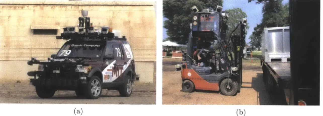
The autonomous vehicle and the forklift shown in Figure 2-1 are robotic vehicles recently developed by the RVSN (Robotics, Vision, Sensor Networks) group at MIT.

A common requirement for each of these vehicles is a map of nearby obstacles to

enable safe navigation. Since different sensors have different perception capabilities and limited fields of view (FOV), each platform has an array of sensors. The Urban Grand Challenge [47] vehicle (Figure 2-1a) has five cameras, 12 planar LIDARs, a 3D Velodyne, and 16 radar sensors. The Agile Forklift [69] (Figure 2-1b) has 4 cameras and 15 planar LIDARs. When combined, the heterogeneous sensors provide a sensing network encompassing the vehicle and work to ameliorate the consequences of any one sensor's failure mode.

The sensors can be considered as a simple kinematic chain, with rigid segments connecting pairs of sensors. In order to combine the information from the various sensors into a single, fused obstacle map, the relative poses of the sensors (i.e., the parameters of each segment) must be known. Thus, we consider the problem of recovering the calibration parameters describing the rigid body transform between sensors.

The 6-DOF calibration task is a common problem (see Section 2.3). Previous approaches typically require manual measurements, establishing a global reference frame, or augmenting the environment with known structure. Instead, we develop a sensor-agnostic calibration process which accepts incremental pose observations and uncertainties as input and produces an estimate of the calibration parameters, along with an uncertainty, as output. Essentially, the estimate is produced by finding the calibration parameters most consistent with the rigid body motion of all the sensors. The technique does not require a special calibration rig, an augmented environment, sensors with overlapping field of views, or synchronous incremental pose observations. Simultaneous Localization and Mapping (SLAM) is not used and no global reference frame must be established.

(19)

(a) _(b)

Figure 2-1: Both these autonomous vehicles require extrinsic sensor calibration to fuse data from multiple sensors.

2.1 Overview

A natural question is whether incremental pose observations alone contain sufficient

information to recover relative sensor calibration. Intuition suggests that such ob-servations are indeed sufficient (Figure 2-2) because the pose difference between two sensors causes them to experience different incremental motion (Figure 2-2b and Fig-ure 2-2c). The calibration that best transforms the motion of the first sensor to align with that of the second sensor will be the desired rigid-body transformation.

We formalize this intuitive argument and develop a procedure to estimate the calibration. We show that the calibration is observable (i.e., that there exists sufficient information in the input observations to estimate the calibration), so long as certain degenerate motion paths are avoided. We explain the Cramer-Rao Lower Bound

(CRLB)

[71]

_{and show how to compute it for the calibration estimate. As we will see,}

the CRLB provides a best-case minimum error (covariance matrix) for the estimate, enabling the accuracy of the calibration to be assessed. The CRLB covariance can also be incorporated, as a source of uncertainty, into subsequent processing.

Our method is applicable to any sensor, or sensor combination, that permits observation of its own incremental motion. The process can also be applied to find the pose of sensors relative to a robot frame, if the relative motion of the robot body can be observed (e.g., using inertial and odometry data). The calibration procedure can be summarized as follows:

1. Move the robot along a non-degenerate path.

2. Recover per-sensor incremental poses and covariances.

3. Resample asynchronous sensor data to correct for different sample times.

4. Use least squares to recover relative sensor calibration.

(20)

p, P2 -P1 p3 P3 -P2 P2 - P1 P3 -P2 (a) (b) (c)

Figure 2-2: As the robot moves from pi to P3, two sensors (positioned as in (a)) will

experience different translational ((b) and (c)) and rotational (not shown) incremental motion. The calibration relating the sensors is the transformation that best brings the disparate observed motions into agreement.

2.1.1 Structure

As suggested in Table 2.1, we separate the discussion between 3-DOF (x, y, 6)

cal-ibration and 6-DOF (X, y, z, p 7, ) calibration. Although 3-DOF calibrations can

be handled by 6-DOF approaches, the 3-DOF case is easier to understand. In the sections describing the 3-DOF calibration, we develop the problem, analyze its observ-ability, and demonstrate our calibration techniques. Subsequent sections discussing the 6-DOF calibration rely on the same underlying theory for parameter recovery, but require a significantly different parametrization. This parametrization, the unit

dual quaternion (DQ), is developed in Sections 2.5.1, 2.5.2, and 2.5.3.

Pseudo-code for the algorithm is initially presented in Section 2.4.6 and developed further thereafter. Additionally, our algorithm can make use of observation uncer-tainties, but these can be difficult to obtain in practice. Therefore, we provide a method to estimate uncertainties in Section 2.4.7. Section 2.4.4 discusses bias in the calibration process.

In the 3-DOF and 6-DOF discussions, we rely on an understanding of estimation and information theory, especially as related to the maximum a posteriori estimator and the CRLB. We review these preliminary concepts in Section 2.2. Previous work on the calibration problem is reviewed in Section 2.3.

(21)

Table 2.1: Calibration outline

3-DOF Calibration 6-DOF Calibration

Problem statement §2.4.1 §2.5.4, §2.5.5 Observability & CRLB §2.4.2 §2.5.6 Estimation §2.4.3 §2.5.7 Interpolation §2.4.5 @2.5.8 Results §2.4.8 §2.5.9

2.1.2 Contributions

1. Sensor-agnostic calibration. Our research is distinct from its predecessors in that we consider the recovery of extrinsic calibration parameters, independent of the type of sensor. We require only that each sensor produce time-stamped data from which its 6-DOF (or planar 3-DOF) incremental motion can be estimated. This incremental motion could be recovered, for example, from image, laser, or

IMU+odometry.

If an uncertainty covariance for these motions is available, it can be incorporated into our estimation procedure. The resulting ability to recover the rigid body transforms between different types of sensors is important because many robotic systems employ a variety of sensors.

2. Automatic parameter recovery. No specific augmentation of the environ-ment or manual measureenviron-ment is required or assumed. Many calibration tech-niques rely on target objects with known characteristics in the sensor's field of view (e.g., fiducials or fixtures). Our calibration procedure, on the other hand, uses only per-sensor ego-motion observations which can often be esti-mated without targets. For example, scan-matching can be used to provide incremental poses without relying on a prepared environment. The result is a greatly simplified and user-independent calibration process.

3. Global reference frame not required. The most common form of calibra-tion proceeds by establishing a global reference frame for each sensor, typically through some form of SLAM or the use of an external network (e.g., GPS). With each sensor localized in a global frame, the rigid body transform best aligning the two frames is the extrinsic calibration. Unfortunately, this method requires either solving the complex SLAM problem before calibration or relying on an external network (which is not always available). Our solution uses only incremental motion and does not require SLAM or an external network. 4. Asynchronous sensor data supported. Sensors are rarely synchronized

(i.e., they do not have the same sampling frequency or phase). Our estima-tor, however, requires incremental motions observed over a common period. Although we can trivially interpolate between observations, we want to do so

(22)

according to the uncertainties of the observations. As a result, we use the Scaled Unscented Transform (SUT) [40] to interpolate sensor data and produce corresponding, resampled noise estimates.

5. Principled noise handling. Most calibration techniques assume all data is

equally accurate, and produce a single set of calibration parameters. A distinct aspect of our calibration algorithm is that it not only accepts both observations and their covariances, but also generates a best-case uncertainty estimate for the calibration parameters. This is an important feature, as degeneracies in the observations have the potential to generate inaccurate calibration parameters if ignored. This inaccuracy can be unbounded due to the degeneracies. By examining the output covariance matrix for singularities, such situations can be avoided.

Furthermore, the calibration is an often ignored source of uncertainty in the system. Small errors in the calibration rotations, for example, can produce significant errors for re-projected sensor data (especially at large distances). By providing an accurate uncertainty estimate, these ambiguities can be accounted for during sensor fusion in a principled way.

2.2 Estimation and Information Theory

In an estimation process, we desire to recover some notion of a true value having made some observations. Estimation theory provides many frameworks enabling estimates to be recovered from observations. Parameter estimation theory, for example, deals with the recovery of values which do not change over time. State estimation theory, on the other hand, enables time-varying values to be recovered. Our sensor calibration task is to estimate a time-invariant, rigid body transform. Accordingly, we focus here only on parameter estimation. (By contrast, the articulated object tracking work in the next chapter performs state estimation.) As we design an algorithm to produce an estimate, we can rely on techniques from information theory to assess the quality of our estimator. Information theory provides tools to answer questions such as:

1. Is it even possible to construct an estimator? We might wish to recover

calibra-tion parameters, but if, for example, our observacalibra-tions are of unrelated quantities (e.g., the weather conditions), we have little hope of success.

2. When will our estimator fail? Even if observations have the potential to enable estimation, there may be special alignments that do not allow it.

3. How good is the output estimate? Assuming it is possible to recover the

(23)

2.2.1 Maximum Likelihood & Maximum a posteriori

Suppose we wish to recover some estimate of parameters, x, given some set of ob-servations, z. For the calibration task, x and z are vectors encoding a series of rigid body transformations. Classically, this problem has been approached from two van-tage points: Bayesian and Non-Bayesian. In the Bayesian approach, the parameters are considered to be random values drawn from some probability distribution, P (x). In the Non-Bayesian approach, an unknown true value of the parameters, xO, is con-sidered to exist.

In the Bayesian approach, we wish to produce an estimate, , , of the parameters which is most likely given the observations. This is known as maximum a posteriori estimation (MAP):

AP (z) = argmax P (x I z) (2.1)

The probability of the parameters given the data, P (x I z), is often difficult to compute because it requires solving an inverse problem (computing parameters from observations). Fortunately, Bayes' rule can be employed:

iMA (Z) = argmax P ZIX ()(2.2) P(z)

= argmax P (z I x) P(x) (2.3)

X

The forward model, P (z I x), represents the probability of some observations given the parameters. Notice that P(z), the probability of a particular set of observations, does not affect the maximization. The probability of some parameters, P(r), on the other hand, requires more careful consideration. From a non-Bayesian approach, P(x) can be considered uniform and removed from the optimization - essentially, every parameter x is considered equally likely. This is known as the maximum likelihood estimator:

±ML (z) argmaxP(zlx) (2.4)

In the MAP, P(x) is modeled explicitly. For example, a Gaussian distribution might be used to calculate the probability of a particular set of calibration parameters. Thus, the MAP and ML estimators differ only in the assumption they make regarding the uniformity of P(x).

2.2.2 The Cramer-Rao Lower Bound

As we might expect, noise at the inputs of the estimator will cause noise at the output. The CRLB describes a lower limit on the noise at the output. That is, if the covariance on the output of an estimator reaches the CRLB, the estimator has

(24)

extracted all available information from the input data. The remaining noise is a function only of the noise on the inputs and cannot be reduced further.

The derivation of the CRLB depends on an assumption that the estimate is un-biased (for our calibration problem, we address the unun-biased nature of our estimator in Section 2.4.4). If the estimator is unbiased, then

E [i (z) - x] = (i (z) - x) P (zlx) dz = 0 (2.5)

Building on this fact, we follow the derivation of the CRLB in [71] for scalar states and observations (later, we extend to the vector case). Taking the derivative of both sides and assuming the derivative of the integrand is integrable, yields:

J(9

(z) - x) P (zlx) dz = 0 (2.6)

((i (z) - x) P (zlx)) dz = 0 (2.7)

-P (zx) + (l (z) - X) P (zlx) dz = 0 (2.8)

Since P (zlx) is a distribution which must integrate to unity, f P (zlx) dz 1, and

(f (z) - x) P (zlx) dz = 1 (2.9)

Noting the definition for the derivative involving a natural logarithm,

am1ny _ lay ay Ylny 8 ,P(z x) = an P (zl)

ax ya ax =anx(z ~x) (2.10)

Then, plugging in to Equation 2.9:

( - X) P (Z) alnP(zx) dz = 1 (2.11)

The Schwarz inequality,

(f

f

(z) g(z) dz)2

< f f(z) 2 _{dz f} g(z) 2 dz can be applied if we factor P (zIx): (((z) - X) VP (z ) (n (zX)aInP zx) dz = 1 (2.12) =f W) zg(z)

f

(z) g (z) dz) = 1 (2.13) (Z) - X) VP (zx)) dz. P (z) n P z

I)

dz (2.14)

(25)

The first term to the right of the inequality is the variance of the estimate:

J

(

(z) - x) /P (z x)) dz =f (j (z) - X)2P (zIx) dz = E

[(i

(z) - X)2] (2.15) And, similarly, for the second term to the right of the inequality:

]/

P(z) In P Ox ax

)

dz =n(' 1( Oz P (zlx) dz (2.16)

=E [(OnP(zlx) 2 (2.17)

Substituting,

1 < E [(j (Z) - X)2] -E On zj (2.18)

var (f (z)) = E [(, (z) - X)2] > E alnP(zlx) (2.19)

We see then that the uncertainty of the estimate, var (ii (z)) , can be no less than:

J= E [(9nPzx

)21

When x and z are vector quantities, the Fisher Information Matrix (FIM), J, is written as:

J = E [(Vx In P (zIx)) (Vx ln P (zIX))T (2.20)

and var (i (z)) > J. Here, as in [2], we abuse notation slightly: A > B is interpreted

as A - B > 0, meaning that the matrix A - B is positive semi-definite. The Vx

operator calculates the gradient of the operand along the direction of x.

We see immediately that if the FIM is non-invertible, then the variance on one or more of our parameters will be unbounded. As a somewhat oversimplified analogy, consider J as a scalar; if J = 2, then the variance must be greater than 1/2. If

J= 0 (corresponding to a rank deficient matrix J), then the variance is infinite. An

infinite variance means that nothing is known about the parameter. Thus - at least intuitively - we can see that if J is rank deficient, we will not be able to estimate x. Throughout the following sections, we will use several terms. First, a system is said to be observable if the corresponding FIM is full rank. This means that a system is observable only if all the output parameters can be determined from the inputs. Later, we will show that, in our setting, the calibration parameters are observable from incremental pose inputs.

An estimator is efficient if it achieves the CRLB. It is not generally possible to show that non-linear transforms (e.g., such as our rigid body transformations) result in estimators which are efficient [71, p71]. However, as demonstrated in Section 2.4.2, our estimator comes close to the CRLB.

(26)

2.3 Background

Ideally, it would be easy to determine the transformation relating any pair of sensors. One could use a ruler to measure the translational offset, and a protractor to measure the orientation offset. In practice, it is rarely so easy. A sensor's coordinate origin typically lies inside the body of the sensor, inaccessible to direct measurement. Curved and textured sensor housings, and obstructions due to the robot itself, usually make direct measurements of sensor offsets difficult or impossible.

Alternatively, one could design and fabricate precision sensor mounts and elimi-nate the calibration problem. While this approach may be practical for small, closely-spaced sensors such as stereo rigs, it would be cumbersome and costly for larger systems. Moreover, the need for machined mounts would hinder field adjustment of sensor configurations.

Figure 2-3: Calibration solutions requiring SLAM attempt to establish a common reference frame for the sensors (blue and red) using landmarks (green).

In light of these practical considerations, we desire a software-only algorithm to estimate calibration using only data easy to collect in the field. One approach would be to establish a common global reference frame, then estimate the absolute pose of each sensor at every sample time relative to that frame. The calibration would then be the transformation that best aligns these poses. For example, in the setting of Figure 2-3, the task would be to find the calibration that aligns the paths of the blue and red sensors, having been estimated from some set of landmarks (green). In practice, however, recovering accurate absolute sensor pose is difficult, either because of the effort required to establish a common frame (e.g., through SLAM), or the error that accumulates (e.g., from odometry or inertial drift) when expressing all robot motions in a common frame.

Any calibration method employing global, metrical reconstruction will necessar-ily invoke SLAM as a subroutine, thus introducing all the well-known challenges of solving SLAM robustly (including data association, covariance estimation, filter con-sistency, and loop closure).

(27)

Researchers have, nevertheless, attempted to recover absolute pose through vari-ous localization methods. Jones [39] and Kelly [45] added calibration parameters to the state of an Extended Kalman Filter and an Unscented Kalman Filter (UKF), respectively. Although the calibration parameters are static, they are expressed as part of a dynamic state. Recognizing this, the authors fix the values after some initial period and prevent further updates. Jones [39] also shows observability; a comparison with our work is provided in Section 2.4.2.4.

Gao [28] proposed a Kalman filter incorporating GPS, IMU, and odometry to estimate a robot's pose. They place pairs of reflective tape, separated by known distances, throughout the environment. These reflectors are easily identified in the LIDAR returns and they optimize over the 6-DOF sensor pose to align the reflector returns. To account for GPS drift, they add DOFs to the optimization allowing the robot to translate at several points during its travel.

Levinson [48] recovered calibration through alignment of sensed 3D surfaces gen-erated from a multi-beam (e.g., Velodyne) LIDAR. Here, the robot's pose is required (e.g., via SLAM) to accumulate sufficiently large surfaces. They extended their work in [49] to calibrate 3D LIDARs and cameras. They do so by correlating depth dis-continuities in the 3D LIDAR data to pixel edges in the images.

Maddern [51] recovers the calibration parameters by minimizing the entropy of point cloud distributions. The authors compute a Gaussian Mixture Model for 3D LIDAR and 2D LIDAR points, then attempt to minimize the Renyi entropy measure for the point cloud. The technique requires a global estimate of the robot's position (e.g., via GPS), but they minimize long-term drift by performing the optimization on subsets of the data.

When it is possible to augment or prepare the environment, absolute pose can also be established with known, calibrated landmarks. For example, Blanco [4] provides sensor datasets with known calibrations to the community. The calibrations for the GPS, LIDARs, and cameras are recovered automatically. For the GPS and LIDAR data, they use SLAM for each sensor and then optimize for the calibrations. For the camera, they rely on known, hand-selected 3D landmarks in the environment. Simi-larly, Ceriani [15] used GPS and calibrated rigs to establish a global sensor reference frame.

As in our work, others have also used incremental poses for calibration. Censi [14] optimizes for several intrinsic parameters (e.g., robot wheel base) and a 3-DOF cali-bration. The authors use scan-matching to determine an incremental pose, then op-timize for the robot's wheel base and a 3-DOF 2D LIDAR calibration. Our method, however, is distinct in that it accounts for observation noise in a principled way.

Boumal [6] investigates recovering incremental rotations. The authors use two Langevin distributions, a rotationally symmetric distribution designed for spherically constrained quantities: one for inliers and one for outliers. Using an initial guess based on the SVD, they show good robustness against outliers.

Incremental motions have also been used to recover "hand-eye calibration" param-eters. The authors in [34, 21, 17, 72] recover the calibration between an end-effector

(28)

and an adjacent camera by commanding the end-effector to move with some known velocity and estimating the camera motion. The degenerate conditions in [17, 72] are established through geometric arguments. We confirm their results via information theory and the CRLB. Further, the use of the CRLB allows our algorithm to identify a set of observations as degenerate, or nearly degenerate (resulting in a large vari-ance), in practice. Dual quaternions have been used elsewhere [21]. We extend this notion and explicitly model the system noise via a projected Gaussian.

2.4 3-DOF Calibration

This section considers the problem of recovering 2D (3-DOF) calibration parame-ters. After formally stating the calibration problem (Section 2.4.1), we show that calibration is observable (Section 2.4.2). We describe the estimation process and bias computation in Section 2.4.3 and Section 2.4.4, respectively. In practice, one typically must (1) interpolate incremental poses (Section 2.4.5) and their associated covariances for asynchronous sensor data and (2) reliably estimate the covariances for relative pose observations for common sensors such as LIDARs (Section 2.4.7). Using simulated and real data from commodity LIDAR and inertial sensors, we demonstrate calibrations accurate to millimeters and milliradians (Section 2.4.8).

Later, in Section 2.5, we consider the full 3D (6-DOF) calibration process. We present the 2D process first, however, because the mathematical analysis, optimiza-tion techniques, and noise model are significantly easier to understand in the 2D case. This section ignores the non-Euclidean nature of SE(2) for simplicity. Later, when we address such issues for SE(3), we realize that similar adjustments are required for

SE(2).

2.4.1 Problem Statement

Our task is to estimate the static calibration parameter vector k =

[x,

YS, Os]

repre-senting the translational and rotational offsets from one sensor, r, to a second sensor, s. Figure 2-4 shows the graphical model [46] relating the variables of interest, with

Vri the latent, true incremental poses of sensor r at time i and zi and zs the

cor-responding observed incremental poses of the sensors. As indicated in the graphical model, the observed incremental poses of both sensors depend only on the calibration and the true motion of one of the sensors. As a result, the true motion of the other

sensor, vsi, need not be estimated.

Figure 2-5 illustrates the system input. In this example, the r and s sensors travel

with the planar robot (left), producing N = 3 incremental pose observations (right).

We define g(-) to relate the true motion of sensor s, vsi, to Vri and the rigid body

transform k:

(29)

Vr1 Vr2

Zrl Zs1 Zr2 Zs2

k

Figure 2-4: Graphical model of calibration and incremental poses is shown.

e Z13 z l rZr3 Zr2 Zs3 zs₁ zs 2

Figure 2-5: Incremental poses for the r (red) and s (blue) sensors are observed as the robot travels. The observations are plotted on the right in x-y-6 coordinates. The true calibration parameters will transform the red and blue observations into alignment.

Again, the true motion of sensor s need not be estimated because it can be

cal-culated from the other estimated quantities. Further, let z, = [zn1, Zr2, -- , ZrN], zS = [zsi, Zs2, * , ZsN], and z = [zr, z,].

Each measurement for the r sensor, Zri, is a direct observation of the latent variable

Vri. Each measurement for the s sensor, zi, is an observation based on its true motion, voi. If the o operator is used to compound rigid body transformations, then:

VSi = g (Vri, k) = k-1 Vri o k (2.22)

Essentially, the g(.) function transforms the incremental motion from the r frame into the s via rotations.

Although we are interested only in the calibration parameters k, the true

incre-mental poses Vr = [Vr, Vr2, * -, VrN] at every sample time are also unknown variables.

The parameters to estimate are x = [Vr, k] = [Vri, Vr2, - - , VrN, Xs, Ys, Os]. This state

(30)

each observation. However, as we demonstrate with real data in Section 2.4.8, the

estimates converge quickly with manageable N; our experiments used N = 88 and

N = 400.

Finally, we define the equations relating the expected observations and true values as:

G(vr,k) = [vr I VrN g(vr1,k) g(vrN,k)] (2.23)

Note that G has dimension 6N x 1.

2.4.2 Observability & the Cramer-Rao Lower Bound

Before attempting to recover the calibration from the observed incremental pose data, we must first show that there exists sufficient information in the observed data to determine the calibration parameters. As described in Section 2.2, such observability is guaranteed when the the CRLB is full rank.

2.4.2.1 The FIM and the Jacobian

If we assume an additive Gaussian noise model, then:

z = G(x) + 6 (2.24)

where 6 ~ N(0, EZ). Alternatively, we can write that P(zlx) - N (G(x), Ez) and

apply Equation 2.20 in order to determine the FlM for the calibration parameters. We assume that the observation covariance, Ez, is full rank. That is, we assume that

all dimensions of the observations are actually measured.

Let y= z - G (x), then Vxy = -JG, where JG is the Jacobian of G. Note that

JG is a function of x, but we eliminate the parameter for simplicity. Then

V, In P (z I x) = V,,ln c exp

(yT

zly)

(2.25)

-1 (T

= V, In (c) + ln exp ( y2 Ez Y) (2.26)

= V ₂1 (yTE-1y) (2.27)

(31)

Substituting into Equation 2.20 and proceeding as in

[75]:

J = E [(V In P (z I X)) (Vx lnP(z x))T] (2.29) = E

[(JrE

ly ) (jT EZly )T (2.30) =

E

J Z lyyT (Z1)T J] _(2.31) = JGj 1E yyT] ( G1)TJ (2.32) jT Z I1x(Z 1)TjG _(2.33) jT (Z)Tj G (2.34) = J -1 JG (2.35)

In Equation 2.32, the expectation is over the observations z, so all the terms except

yyT factor. In Equation 2.33, we make use of the fact that E [yyT] = Ez by definition. As we examine the degenerate conditions, we will be interested in the rank(J). If we factor Ez using, for example, the Cholesky factorization, such that E; LLT,

then:

rank(J) = rank(J E;1 JG) (2.36)

= rank (JGTLLT JG) (2.37)

= rank((LT JG)T (L JG)) (2.38)

= rank (L T

JG) (2.39)

= rank(JG) (2.40)

We can restate Equation 2.35 as follows: if the observation noise has a Gaussian distribution, then the FIM can be calculated as a function of the observation Jacobian and observation covariance. This has two important implications:

1. Given the covariance and having computed the Jacobian, we have the quantities needed to calculate a lower bound on the noise of our estimate (Equation 2.35). 2. As shown in Equation 2.40, J has full rank if and only if JG has full column rank. Thus, by analyzing the column rank of JG, we can determine whether the calibration is observable.

2.4.2.2 The FIM Rank

First, consider the case where there is one incremental pose observation for each

sensor, i.e., z = [Zi, ZsI] = [Z,1r, zri, , zsix, zsiy, zsi]. _{The parameter vector is}

then x = [vr, k] = [vrix, Vrly, VrlO, xs, ys, 0,]. The resulting 6 x 6 Jacobian matrix of Equation 2.23 has the form below. This matrix is clearly rank-deficient because rows

Articulated pose estimation via over-parametrization and noise projection