HAL Id: hal-00401752
https://hal.archives-ouvertes.fr/hal-00401752
Submitted on 6 Jul 2009
HAL is a multi-disciplinary open access
archive for the deposit and dissemination of
sci-entific research documents, whether they are
pub-lished or not. The documents may come from
teaching and research institutions in France or
abroad, or from public or private research centers.
L’archive ouverte pluridisciplinaire HAL, est
destinée au dépôt et à la diffusion de documents
scientifiques de niveau recherche, publiés ou non,
émanant des établissements d’enseignement et de
recherche français ou étrangers, des laboratoires
publics ou privés.
Identifiable parameters for parallel robots kinematic
calibration
Sébastian Besnard, Wisama Khalil
To cite this version:
Sébastian Besnard, Wisama Khalil. Identifiable parameters for parallel robots kinematic calibration.
ICRA-IEEE Robotics and Automation Conference, 2001, Seoul, South Korea. pp.2859-2866.
�hal-00401752�
Identifiable Parameters for Parallel Robots Kinematic Calibration
S. BESNARD, W. KHALIL
Institut de Recherche en Communications et Cybernétique de Nantes, U.M.R. CNRS 6597 1, rue de la Noë, B.P. 92101 F-44321 Nantes Cedex 3, France
Abstract
This paper presents a numerical method for the determination of the identifiable parameters of parallel robots. The special case of Stewart-Gough 6 degrees-of-freedom parallel robots is studied for classical and self calibration methods, but this method can be generalized to any kind of parallel robot. The method is based on QR decomposition of the observation matrix of the calibration system. Numerical relations between the identifiable and non identifiable parameters can be obtained.
1. Introduction
The classical methods for parallel robot calibration need external sensors to measure the position and orientation of the mobile platform [1] [2] [3] [4] [5]. The calibration problem is formulated in terms of minimizing the difference between the measured and computed motorized joint variables, it uses the inverse kinematic model which is easy to calculate for parallel robots. Self calibration methods using extra sensors on the passive joints have been also proposed for parallel robots [6] [7] [8] [9]. These methods are based on the use of redundant sensors on the passive joints and to adjust the values of the kinematic parameters in order to minimize a residual between the measured and the calculated values of the angles of these joints. As many parallel robots don’t have redundant sensors on the passive joint, mechanical constraints on the leg can also be used [10] [11].
For some calibration methods, all the geometric parameters cannot be identified. In previous work, the identifiable parameters of parallel robots are derived by intuition. In the case of serial robots, the identifiable parameters are computed from a QR decomposition of the analytical observation matrix [12]. We propose to extend this method for parallel robots even in the case where the Jacobian matrix cannot be obtained analytically.
2. Description of the robot
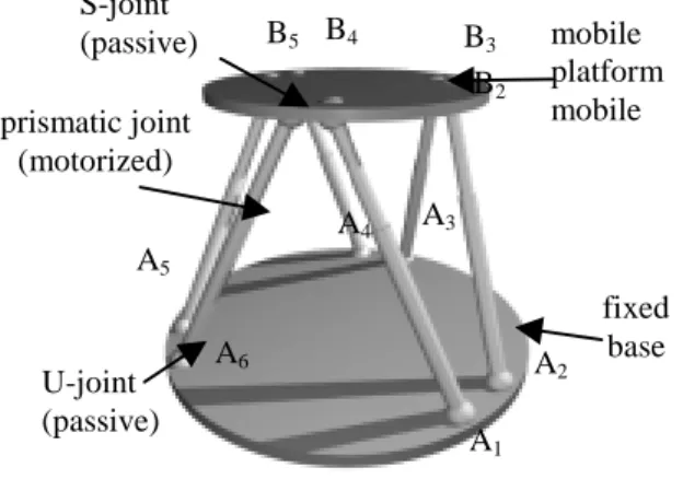
The parallel robot studied here is the Stewart-Gough 6 degrees of freedom robot (Figure 1). The base
connections are composed of Universal joints (U-joints) and the platform connections are composed of Spherical joints (S-joints). The centers of the U-joints and S-joints are denoted by Ai and Bi (i = 1 to 6) respectively. The
configuration of the parallel robot is given by the (6x1) vector L representing the leg lengths AiBi for i=1,…,6:
L = [ l1 l2 l3 l4 l5 l6 ]T (1-a)
Typically each variable is given as:
i off i
i q q
l = + , (1-b)
where qi is the prismatic position sensor reading and qoff,i
is a fixed offset value.
A1 A2 A3 A4 A5 A6 B2 B3 B4 B5 mobile platform mobile fixed base prismatic joint (motorized) S-joint (passive) U-joint (passive)
Figure 1: Stewart-Gough parallel robot
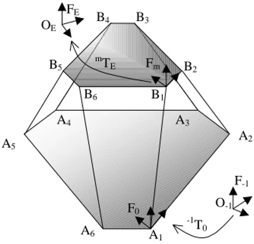
Let the frame F0 be fixed with respect to the base and
frame Fm fixed to the movable platform, such [7]:
- A1 is the origin of frame F0, while the x0 axis is
determined by (A1A2) and x0y0 plane is determined by the
points A1, A2 and A6.
- similarly, B1 is the origin of frame Fm, while B1B2
represents its xm axis and B1B2B6 its xmym plane.
With this definition of F0 and Fm we have: 0Px
mPx
B1 = mPyB1 = mPzB1 = mPyB2 = mPzB2 = mPzB6 = 0
Where jPPi denotes the coordinates of the point Pi with
respect to coordinate system Fj and: jP
Pi = [ jPxPi jPyPi jPzPi ]T
Thus, the robot is described by 24 constant parameters which may be not equal to zero.
A1 A6 A5 A4 A3 A2 B1 B6 B5 B4 B3 B2 Fm F0 FE F-1 -1 T0 m TE OE O-1
Figure 2: Definition of the frames
The (4x4) transformation matrix between frames F0 and
Fm giving the location (position and orientation) of the
platform with respect to the base is denoted by:
0T m = 1 0 0 0 P A m 0 m 0 (2)
The location of frame F0 with respect to the world
reference frame F-1 of the environment is given by a
transformation matrix Z. In addition, the matrix E denotes the location of the end-effector frame FE in frame Fm (cf.
Figure 2). The location of the end- effector frame relative to the world reference frame is:
E T Z T m 0 E 1 = ⋅ ⋅ − (3)
Thus, the coordinates of Ai relative to frame F-1 are:
⋅ = ⋅ = − − 1 P Z 1 P T 1 P i i i A 0 A 0 0 1 A 1 (4)
The coordinates of point Bi relative to frame FE are:
⋅ = ⋅ = 1 P E 1 P T 1 P i i i B m B m m E B E (5)
The matrices Z and E can be defined using 6 independent parameters. Thus, we can describe the geometry of the robot using 36 constant parameters: either by –1PAi and EP
Bi, or by 0PAi, mPBi and the matrices E and Z. The total
number of parameters is thus equal to 42, after taking into account the 6 joint variables.
For the calibration, we propose to use the coordinates of points Ai and Bi in frames F-1 and FE respectively in order
to have homogeneous parameters to identify (only lengths). From these coordinates, it is easy to find the transformations Z and E, and the coordinates of the points of the base and the platform in frames F0 and Fm.
2.1 Kinematic modeling
The inverse kinematic model (IKM) which computes the leg lengths vector for a desired -1TE is unique and easy to
obtain [13]. While, the direct kinematic model (DKM), which gives the matrix -1TE as a function of a given leg
lengths vector, is difficult to obtain analytically and up to 40 solutions may exist [14]. A numerical iterative method based on the inverse Jacobian matrix is used to find a local solution for the DKM.
3. General calibration models
The aim of the kinematic calibration is to estimate accurately the geometric parameters. All the calibration methods are based on calculating a function, for sufficient number of configurations, in terms of the robot parameters and some external variables. The model parameters are estimated by minimizing this function by solving a nonlinear system of equations. The general form of the calibration equation is:
1 1 1 e e e f ( , , ) F( , , ) 0 f ( , , ) q x Q X q x η η η = = ! (6)
where η denotes the geometric parameters, Q={ q1,…, qe }T contains the prismatic positions of the robot for e different configurations, and X = { x1,…, xe }T are the corresponding external measured variables such as the Cartesian coordinates. This nonlinear optimization problem can be solved by the leastsq function of Matlab based on the Levenberg-Marquardt method.
Supposing that the U- and S-joints are perfect, we have to identify the error ∆-1PAi, ∆
E
PBi, ∆qoff,i (with i = 1,…,6).
They will be collected in the vector ∆η. Before solving the calibration equation, it is important to define the identifiable parameters, because only these parameters can
be identified without ambiguity. We propose to determine these parameters using QR decomposition of the observation matrix of the linearized model of randomly e configurations satisfying the constraints of the calibration procedure. The outlines of this algorithm is given references[12,15]. The linearized equations corresponding to the nonlinear equation (6) can be written as:
) W(Q, ) , (Q, η = η ⋅∆η+ρ ∆Y X (7)
where ∆Y is the difference between the model and the real
robot, W is the (r , np) observation matrix of the system, with np the number of geometric parameters and r >> np, The vector ρ indicates the residual errors owing to noise or modeling errors.
For parallel robots, the observation matrix W can be obtained analytically for the calibration method which is based on the IKM. For all the other methods we have to calculate W numerically by supposing small variations ε on each geometric parameter and calculating the corresponding ∆Yi. The jth column of W corresponding to that parameter will be computed as ∆Yj/ε . Good results
are obtained with ε = 10-6 meter for each parameter. The number of the identifiable parameters denoted by b. The QR decomposition will provide as a set of identifiable parameters those corresponding to the first b independent columns of W. We assign a priority number to each parameter, the parameters with higher priority will be placed at first in η. We place at first the offsets qoff,i
(priority 3), and we place at the end the 12 coordinates of the points defining frames F0 and Fm (-1PxA1, -1PyA1, -1 PyA2, -1 PzA1, -1 PzA2, -1 PzA6, E PxB1, E PyB1, E PyB2, E PzB1, EPz
B2, EPzB6) (priority 1), the other parameters will get
priority 2 and will be placed after the offset parameters in the following order:
-1Px
A2,…, -1PxA6, -1PyA3,…, -1PyA6, -1PzA3,…, -1PzA6, then EPx
B2,…, EPxB6, EPyB3,…, EPyB6, EPzB3,…, EPzB6.
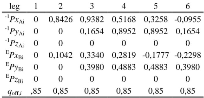
4. Application to calibration methods
We compute the identifiable parameters for several calibration methods for the parallel robot whose nominal parameters are given in Table 1. The obtained identifiable parameters are valid for any robot of the Stewart-Gough type. The grouping relations of the non identifiable parameters are functions of the numerical values of the geometric parameters. leg 1 2 3 4 5 6 -1Px Ai 0 0,8426 0,9382 0,5168 0,3258 -0,0955 -1Py Ai 0 0 0,1654 0,8952 0,8952 0,1654 -1Pz Ai 0 0 0 0 0 0 EPx Bi 0 0,1042 0,3340 0,2819 -0,1777 -0,2298 E PyBi 0 0 0,3980 0,4883 0,4883 0,3980 EPz Bi 0 0 0 0 0 0 qoff,i ,85 0,85 0,85 0,85 0,85 0,85
Table 1: Nominal values of the geometric parameters
4.1 Calibration using the IKM
Measuring the location of the platform, the inverse kinematic model (IKM) can be used to compute the 6 leg lengths of the robot. The calibration method consists in minimizing the residual between the computed and the measured prismatic variables [2].
The equation for each leg and each configuration is:
(
)
(
)
∆ ∆ ∆ − − − − − − = ∆ − − − − − − − − i i i i q L L q , off B E A 1 T E 1 T E 1 B E E 1 A 1 T E 1 B E E 1 A 1 i i i i i i P P . A . P P . A P P P . A P 1 (8) Applying this equation for the 6 legs of the robot and e configurations, we have the relation:η
η ∆
=
∆Q W( X, ). (9)
where ∆Q is the difference between the measured
prismatic joint values and those computed by the IKM. Note that the observation matrix W can be computed analytically. Using (9) for e random configurations, with
e >> 7 such that the number of rows of W is greater than
the number of the parameters. The rank of the matrix W is 42. Thus, all the parameters can be identified. The condition number of W can be used as a measure of the excitation of the parameters by the calibration method. Using e configurations such that the number of equations is 4 times the number of parameters we find that The condition number of W is about 350.
4.2 Calibration with measurement of the position of the platform
Measuring only the position of the platform, we cannot use the IKM of the robot since we have only 3 equations to solve a system of 6 unknowns (the 6 leg lengths of the
robot). Nevertheless, using the direct kinematic model (DKM), if we consider a configuration q of the robot and
pE the measured position of the effector in frame F-1, we
can write the nonlinear model of calibration as:
1
E E
P ( , )qη p 0
− − = (10)
The corresponding linear differential model is:
η
η ∆
Ψ =
∆pE (q, ). (11)
The Jacobian matrix Ψ is obtained numerically by supposing small variation on each parameter and calculating the corresponding variation on ∆pE.
Measuring the position of the end-effector for a sufficient number e of random configurations (minimum 14 configurations), we have: η η η η η ∆ = ∆ Ψ Ψ = ∆ ∆ = ∆ . W( , ). ) , ( ) , ( 1 1 1 E E Q q q p p P e e e ! ! ΕΕΕΕ (12)
The rank of the matrix W is obtained as 39. The identifiable parameters of the system are obtained by the
QR decomposition of this matrix. Applying the rules of
priority described in section 3, the errors ∆EPyB2, ∆EPzB2
and ∆EPzB6 are not identifiable and their effect are
grouped on the other parameters which defines the positions of the S-joints on the mobile platform. We propose to fixe these parameters such that:
0 6 2 2 B E B E B E = = = Pz Pz Py (13)
This makes that the orientation of frame E, which cannot be determined, is such that the x axis is along the measured point and the point B2 while the xy plane is
along the measured point and the points B2 and B6. The
condition number of the observation matrix W for this calibration method using a number of equations which is equal to 4 times the number of parameters is about 2000.
4.3 Calibration using two inclinometers
In this calibration method the rotation angles of the platform of the robot about xm and ym axis are measured
by two inclinometers fixed on the platform [5]. For a given configuration q, the theoretical values α1 and α2 of the inclinometers can be computed using the DKM. These values are functions of some elements of the orientation matrix –1AE and of the angle γ between the inclinometers
axes. The linear differential model can be written as:
η γ η
Φ =Ψ ∆
∆ (q, , ). (14)
where ∆Φ is the difference between the inclinometers measured values Φm and those computed by the model Φ, and Ψ is the numerical Jacobian matrix (cf. section 3). Using a sufficient number e of configurations:
η γ η Φ Φ ∆ ⋅ = ∆ ∆ ) , , W( 1 Q e (15)
The rank of W is 36, there are 4 non identifiable parameters concerning the U-joints (∆-1PxA1, ∆-1PyA1, ∆-1
PzA1 and ∆ -1
PyA2) and 3 on the position of the S-joints
(∆EPxB1, ∆EPyB1 and ∆EPzB1). The effect of these
parameters are grouped on the other parameters of the base (U-joints) and the platform (S-joints) respectively. These results are confirmed by the study of the geometry of the system. The position coordinates of the inclinometers on the platform have no effect. Consequently, we can consider that the origin OE, which
cannot be determined by this method, is aligned with the origin of frame Fm. Then we have by convention:
0 1 1 1 B E B E B EPx = Py = Pz = (16)
Similarly, the position of the base of the robot with respect to F-1 has no influence on the inclinometers
measurement, as well as its orientation around the vertical axis. We can define arbitrarily the origin of frame F-1 as
A1 and the axis x-1 and z-1 such that A2 is in the plane
(A1x-1z-1). Then we have by definition:
0 2 1 1 1 A -1 A -1 A -1 A -1 = = = = Py Pz Py Px (17)
The condition number of the linear observation matrix W for this method using a number of equations which is equal to 4 times the number of parameters is about 2000.
4.4 Calibration with mechanical constraints on the orientation of the legs
This method uses the variables of the motorized prismatic joints corresponding to configurations where either one U-joint or one S-U-joint is fixed by mechanical lock, thus the leg direction is constant with respect to the base or with the movable platform [11].
Each U-joint i is described by 2 angles θ1,i and θ2,i, while each S-joint i is defined using three angles θ3,i, θ4,i and θ5,i.
For a given configuration q, these angles can be computed by a generalized direct kinematic model [11]:
) , ( , 2 , 1 η θ θ q g y i i ui = = (18), ( , ) , 5 , 4 , 3 η θ θ θ q h y i i i si = = (19)
4.4.1 Fixing the U-joint of a leg
Supposing 2 configurations qa and qb for which the ith U-joint has been locked. The nonlinear error function between them is given as yua(qa,η)−ybu (qb,η)=0
i i
The differential equation is given as:
η η ⋅∆ Ψ = − = ∆yu yua yub (q, ) i i i (20)
With a sufficient number e of configurations:
η η ⋅∆ = − − = ∆ ∆ = − − ) , ( W 1 2 1 1 1 Q y y y y y y C e u e u u u e u u u i i i i i i i ! ! (21)
The rank of W is 29, giving 7 non identifiable parameters of the base and 6 non identifiable parameters for the platform. The interpretation of this result is given in section 4.4.4. The condition number of the observation matrix for this method using a number of equations 4 times the number of parameters is about 2500.
4.4.2 Fixing the S-joint of a leg
Using a set of configurations Q = { q1,…,qe } for which the ith S-joint has been locked, we can write a differential linear system of equations by the use of relation (19):
η η ⋅∆ = − − = ∆ ∆ = − − ) , ( W 1 2 1 1 1 Q y y y y y y C e s e s s s e s s s i i i i i i i ! ! (22)
The rank of W (which is computed numerically) is 29, this gives 6 non identifiable parameters for the base and 7 non identifiable parameters for the platform. The condition number of the linear observation matrix W for this calibration method using a number of equations which is equal to 4 times the number of parameters is about 7500.
4.4.3 Mixing the data of locking different joints
If two or more sets of configurations are used, where in
each set either an U-joint or a S-joint has been fixed, the rank of the numerical observation matrix W of the calibration system is 30. The QR decomposition of this matrix shows that 6 parameters of the base and 6 parameters of the platform are not identifiable. With the priority rules, defined in section 3, these parameters correspond to those which define the base and the end-effector transformation matrices Z and E. In practice we put them equal to zero:
0 6 2 2 1 1 1 A -1 A -1 A -1 A -1 A -1 A -1 = = = = = = Pz Pz Py Pz Py Px (23) 0 6 2 2 1 1 1 B E B E B E B E B E B E = = = = = = Pz Pz Py Pz Py Px (24)
This gives: frame F-1 = F0 and Fm = FE.
The condition number of the observation matrix W for this method using a number of equations which is equal to 4 times the number of parameters is about (with one U-joint and one S-U-joint locked) using four time the number of equations that are necessary is about 700.
4.4.4 Comments
This autonomous method cannot identify the Z and E elements because they have no effect on the angles of the legs with respect to the base or the platform. Thus, the maximum number of identifiable parameters by such autonomous calibration method is 30.
When only one set of configurations is used with one U-joint (respectively one S-U-joint) locked, a 7th geometric parameter of the base (respectively of the platform) cannot be identified. In fact, placing the center of the locked joint along its leg direction will satisfy the locking constraint (cf. figure 3). That is why we have a non identifiable parameter more. This situation has not been mentionned in reference [11], but it has been shown that two different joints must be locked to get good results.
4.5 Calibration with sensors on Universal joints
Zhuang [9] has presented autonomous methods based on the use of extra sensors on some passive U-joints. Knowing a set of e random configuration Q and the real (measured) values of θ1,i and θ2,i of U-joint i for each configuration, the following linear differential system can be written from (18):
( )
( )
= η ⋅∆η − − ) , ( W r 1 r 1 Q y y y y e u e u u u i i i i ! (25)where
( )
r 1i u
y is the vector of the values measured for the ith U-joint and 1
i u
y is computed from the DKM.
constrained leg
2 positions for the U-jo int
Figure 3: Two different robots with the same orientation of one leg for a given configuration q
The QR decomposition of W shows that using only one sensor reading is sufficient to identify 30 parameters which is the maximum for a self calibration method. In this case, the condition number of W is about 1500. This means that the increase of the number of measured angles increases the observability of the system, using 6 sensors on 3 passive U-joint gives reduces the condition number to about 350.
5. Conclusion
This paper presents a generalized method which gives the identifiable and non identifiable geometric parameters for the calibration methods of parallel robots. This method is based on the QR decomposition of a numerical observation matrix of the calibration system which is obtained numerically by supposing small variations on each geometric parameter of the model. Results are given for several methods, the physical interpretation of the non identifiable parameters has been given. The observability measure of each method is given by the condition number of the observation matrix of the linearized model.
References
[1] O. Masory, J. Wang and H. Zhuang, "On the accuracy of a Stewart platform - Part II, Kinematic calibration and compensation,” in Proc. IEEE Int.
Conf. on Rob. and Aut., 1993, pp.725-731.
[2] H. Zhuang, O. Masory and J. Yan, "Kinematic
calibration of Stewart platforms using pose measurements obtained by a single theodolite,” in
Proc. of IROS 1995, pp.329-335.
[3] H. Zhuang, J. Yan and O. Masory, "Calibration of Stewart platforms and other parallel manipulators by minimizing kinematic residuals,” J. of Rob. Systems,
15, 7, pp.395-405, 1998.
[4] P. Vischer and R. Clavel, "Kinematic calibration of the parallel Delta robot," Robotica, 16, pp.207-218, 1998.
[5] S. Besnard and W. Khalil, "Calibration of parallel robots using two inclinometers", in Proc. IEEE Int.
Conf. on Rob. and Aut., 1999, pp.1758-1753.
[6] C.W. Wampler, J.M. Hollerbach and T. Arai, "An implicit loop method for kinematic calibration and its application to closed-chain mechanisms," IEEE
Trans. on Rob. and Aut., 11, 5, pp.710-724, 1995.
[7] H. Zhuang and L. Liu, "Self calibration of a class of parallel manipulators," in Proc. IEEE Int. Conf. on
Rob. and Aut., 1996, pp.994-999.
[8] A. Nahvi, J.M. Hollerbach and V. Hayward, "Calibration of a parallel robot using multiple kinematic closed loops," in Proc. IEEE Int. Conf. on
Rob. and Aut., 1994, pp.407-412.
[9] H. Zhuang, "Self calibration of parallel mechanisms with a case study on Stewart platforms," IEEE
transaction on Rob. and Aut.,13,3, pp.387-397, 1997.
[10] P. Maurine, K. Abe and M. Uchiyama, "Towards more accurate parallel robots," in IMEKO-XV, 15th
World Congress of Int. Measurement Confederation,
Osaka, Japan, 10, 1999, pp.73-80.
[11] W. Khalil and S. Besnard, "Self calibration of Stewart-Gough parallel robots without extra sensors,"
IEEE transaction on Rob. and Aut., 15, 6,
pp.1116-1121, 1999.
[12] W. Khalil, S. Besnard, Ph. Lemoine, "Comparison study of the geometric parameters calibration methods ", Int. Journal of robotics and Automation, ", Vol. 15, No. 2, pp. 56- 67, 2000,
[13] J.P. Merlet, "Les robots parallèles," Traité des
Technologies Nouvelles, Série Robotique, Hermès
Ed., Paris, 1997.
[14] M.L. Husty, "An Algorithm for solving the direct kinematic of Stewart-Gough-type platforms," in Proc
ARK, Ljubljana, Slovania, 1994, pp.449-458.
[15] W. Khalil, S. Besnard, Ph. Lemoine,, "Gecaro: A system for the geometric calibration of robots", APII-Jesa, Vol.33, n°5-6 juillet, 1999, pp.717-739.