HAL Id: hal-00007594
https://hal.archives-ouvertes.fr/hal-00007594
Submitted on 20 Jul 2005
HAL is a multi-disciplinary open access
archive for the deposit and dissemination of
sci-entific research documents, whether they are
pub-lished or not. The documents may come from
teaching and research institutions in France or
abroad, or from public or private research centers.
L’archive ouverte pluridisciplinaire HAL, est
destinée au dépôt et à la diffusion de documents
scientifiques de niveau recherche, publiés ou non,
émanant des établissements d’enseignement et de
recherche français ou étrangers, des laboratoires
publics ou privés.
Site testing in summer at Dome C, Antarctica
Eric Aristidi, Abdelkrim Agabi, Eric Fossat, Max Azouit, Francois Martin,
Tatiana Sadibekova, Tony Travouillon, Jean Vernin, Aziz Ziad
To cite this version:
Eric Aristidi, Abdelkrim Agabi, Eric Fossat, Max Azouit, Francois Martin, et al.. Site testing in
summer at Dome C, Antarctica. Astronomy and Astrophysics - A&A, EDP Sciences, 2005, 444,
pp.651. �10.1051/0004-6361:20053529�. �hal-00007594�
ccsd-00007594, version 1 - 20 Jul 2005
(DOI: will be inserted by hand later)
Site testing in summer at Dome C, Antarctica
E. Aristidi
1, A. Agabi
1, E. Fossat
1, M. Azouit
1, F. Martin
1, T. Sadibekova
1, T. Travouillon
2, J. Vernin
1, and A. Ziad
11 Laboratoire Universitaire d’Astrophysique de Nice, Universit´e de Nice Sophia Antipolis, Parc Valrose, 06108 Nice Cedex 2,
France
2 School of Physics,University of New South Wales, Sydney, NSW 2052, Australia
Received: May 2005 / Accepted:
Abstract.We present summer site testing results based on DIMM data obtained at Dome C, Antarctica. These data have been collected on the bright star Canopus during two 3-months summer campaigns in 2003-2004 and 2004-2005. We performed
continuous monitoring of the seeing and the isoplanatic angle in the visible. We found a median seeing of 0.54′′and a median
isoplanatic angle of 6.8′′. The seeing appears to have a deep minimum around 0.4′′almost every day in late afternoon.
Key words.Site Testing, Antarctica
1. Introduction
The French (IPEV) and Italian (ENEA) polar Institutes are constructing the Concordia base on the Dome C site of the Antarctic plateau (75S, 123E), at an elevation of 3250 m, that corresponds, given the cold air temperatures, to an air pressure encountered around 3800 m at more standard latitudes. The Concordia construction is now completed, the first winterover has started in 2005. Astronomy is obviously near the top of the list of the scientific programmes that will benefit of this unique site: the extremely cold and dry air is complemented by very low winds, both at ground level and at higher altitude, so that an exceptionally good seeing is expected.
In the late 90’s a site testing program based on balloon-borne microthermal sensors has been conducted by J. Vernin and R. Marks at South Pole (Marks et al. 1999). As katabatic winds are present at South Pole, these authors found poor see-ing from the ground (recent measurements by Travouillon et al. (2003) confirmed a value of 1.7′′in the visible range). An
amazing result is that the seeing drops down to 0.3′′at 200 m
height above the surface, i.e. at an altitude of 3050 m above the sea level. Therefore Dome C with its 3250 m altitude and located in a low wind area, appeared as an excellent candidate for astronomy.
These promising qualities encouraged our group to initi-ate a detailed analysis of the astronomical site properties. In 1995, a Franco-Italian group directed by J. Vernin made a pio-neering prospective campaign at Dome C and launched a few meteorological balloons. A systematic site testing program was then initiated, under the name of Concordiastro, first funded by IPEV in 2000. Proposed site testing was based upon two kinds of measurements. First, a monitoring of the turbulence
param-Send offprint requests to: E. Aristidi, e-mail: [email protected]
eters in the visible (seeing r0, isoplanatic angle θ0, outer scale
L0 and coherence time τ0) with a GSM experiment (Ziad et
al. 2000) specially designed to work in polar winter conditions. In addition to this monitoring, it was proposed to launch bal-loons equipped with microthermal sensors to measure the ver-tical profile of the refractive index structure constant C2
n(h)
(Barletti et al. 1977). 50 to 60 balloons were foreseen to be regularly launched during the polar winter.
On-site campaigns began in summer 2000-2001 and were performed every year until 2004-2005 with a double aim. It was first necessary to test the behaviour of all instruments in the “intermediate” cold temperature of the summer season, ranging between -20 and -50◦C. This first step was also used to
antic-ipate the more difficult winter conditions, with -50 to -80◦C,
for being technically confident with the first winterover equip-ment. On the other hand, the summertime sky quality is inter-esting in itself as solar observations were started in 1979-1980 at the South Pole. At Dome C the long uninterrupted sequences of coronal sky (far longer than at South Pole) and the expected occurrence of excellent seeing make it a very promising site for high resolution solar imaging and specially solar coronography. So far 6 summer campaigns have been performed totalling 80 man-week of presence on the site. The first winterover has also begun this year. 197 meteorological balloons have been successfully launched, corresponding results have been pub-lished in Aristidi et al. (2005). Major conclusions are that the wind speed profiles in Dome C appears as the most stable among all the astronomical sites ever tested, and that the ma-jor part of the atmospheric turbulence is probably generated in the first 100 m above the snow surface, where the temperature gradients are the steepest (around 0.1◦C/m).
In this paper we present the results of daytime turbulence measurements (seeing and isoplanatic angle) made with
vari-2 E. Aristidi et al.: Site testing in summer at Dome C, Antarctica
ous techniques. The paper is organised as follows: in Sect. 2 we briefly review the theory of the turbulence parameters we mea-sured. Section 3 presents the instrumental setup at Dome C. Section 4 describes the observations, the various calibration procedures and the online and offline data processing. The
re-sults of the monitoring are in Sect. 5. A final discussion is presented in Sect. 6 and an appendix on error analysis ends the paper.
2. Theory
2.1. Seeing
Atmospheric turbulence is responsible for the degradation of image resolution when observing astronomical objects. The full width at half maximum (FWHM) of the long-exposure point-spread function broadens to a value ǫ called seeing, usu-ally expressed in arcseconds, this parameter represents the an-gular resolution of images for given atmospheric conditions. In the visible ǫ is around 1′′for standard sites.
Fried (1966) introduced a so-called parameter r0 that can
be regarded as the diameter of a telescope whose Airy disc has the same size than the seeing. He derived the following relation ǫ =0.98 λ
r0 (1)
The seeing is one of the most important parameters that de-scribes atmospherical turbulence. Seeing monitors have been installed in major observatories such as ESO Paranal and pro-duce constant data that are used to optimize the observations. Seeing estimation can be made by various methods (Vernin & Munoz 1995); seeing monitors that allows continuous mea-surements are traditionally based on differential image motion such as the DIMM (Differential Image Motion Monitor) used at Dome C. It is extensively described in the literature (Sarazin & Roddier 1990, Vernin & Munoz 1995, Tokovinin 2002) and has become very popular because of its simplicity.
A DIMM is a telescope with an entrance pupil made of 2 diffraction-limited circular sub-apertures of diameter D < r0,
separated by a distance B > D. A tilt is given to the light propagating through one of the two apertures to produce twin images that move according to the turbulence. Fried param-eter is computed from longitudinal (σ2l) and transversal (σ2t)
variances of the image motions using equations 5 and 8 of
Tokovinin (2002).
2.2. Isoplanatic angle
The isoplanatic angle is a fundamental parameter for adaptive optics (AO). It is the correlation angle of the turbulence, i.e. the maximum angular distance between two point-sources affected by the same wavefront distortions. In AO systems, these dis-tortions are usually estimated on a nearby bright reference star. This reference star must be in the isoplanatic domain, which in most cases reduces dramatically the observable piece of sky.
As for the seeing, the isoplanatic angle θ0 is a scalar
ran-dom variable, usually expressed in arcseconds, resulting from an integral over the C2
n profile (Ziad et al. 2000, Avila et al.
Fig. 1. Concordiastro observatory in November 2004. One can
see the two platforms and the wooden igloo between. The DIMM is on the top of one platform.
1998). Loos & Hogge (1979) proposed an approximate estima-tion based on the scintillaestima-tion of a point-source star through a 10 cm pupil. Estimation is even better if one uses a 4 cm diame-ter central obstruction. As for the DIMM, this technique allows a continuous monitoring of the isoplanatic angle as well as the scintillation data. It is used routinely by the GSM instrument (Ziad et al. 2000) for site qualification.
3. Instrumentation
3.1. The Concordiastro observatory
The Concordiastro observatory is based on two wooden plat-forms designed by J. Dubourg (Observatoire de la Cˆote d’Azur) and built by the “Ateliers Perrault Fr`eres”, a factory of west-ern France. The design of these platforms recalls the first floor of the Eiffel Tower (see Fig. 1). These platforms are 5 m high and equipped with massive supports for the telescopes. The height has been chosen for site-testing purpose to avoid the surface layer turbulence. They are located 300 m away of the Concordia station, in South-West direction to avoid pollu-tion (wind comes from South or South-West most of the time (Aristidi et al. 2005)). The first one was erected in December 2002, the second one in January 2004. All the installation is built onto a 2 m high pavement of compacted snow for stability (the same kind of pavement that supports the Concordia build-ings).
Between the two platforms, a wooden container nicknamed “igloo” hosts the electronics and the control systems. It was installed at the very end of the 2003-2004 summer campaign. It is cabled to the telescopes, and a fiber optic link is foreseen for remote control from Concordia towers during the winter.
Additional telescopes have been installed at 1.50 m above the ground during the campaign 2004-2005 for estimating the surface layer contribution in the seeing.
Table 1. Technical specifications of the CCD camera
Number of pixels: 640× 480
Pixel size: 9.9× 9.9µm
Binning modes: horizontal: 1,2
vertical: 1,2, 4
Dynamic range: 12 bits
Exposure time: 10µs to 10 s
Frame rate 40 fps without binning
76 fps in binning 2× 2 Maximum QE 40% at 350 and 500 nm Bandwith (FWHM) 320 – 630 nm ADU 7 e−/count Readout noise: 16 e− 3.2. Telescopes
We use Schmidt-Cassegrain Celestron C11 telescopes (diam-eter 280 mm) with a×2 Barlow lens (equivalent focal length 5600 mm). Optical tubes have been rebuilt in INVAR to reduce thermal dilatations (these dilatations cause defocus since they change the distance between the primary and secondary mir-rors). Several technical improvements have been made on the primary mirror support, and the grease of the focus system have been replaced by a cold-resistant one (up to -90◦C).
These telescopes are placed on equatorial mounts Astro-Physics 900. Here again, some customization has been per-formed: grease was changed and heating systems were placed in the motor carters. Tracking has worked successfully during the entire polar summers. The mounts are placed on massive wooden feet fixed to the platform. Polar alignment is made by Bigourdan’s method on solar spots (fortunately we were close to a solar maximum and finding spots had never been a prob-lem), then on Venus, and fine tuning was made on Canopus itself during the observations.
3.3. Cameras
At the focus of all our telescopes we use a digital CCD cam-era (PCO Pixelfly) connected to a PCI board via a high speed transfer cable. Technical specifications are given in Table 1. The camera was placed into an insulated and thermally con-trolled box, insulation being inherited from spatial technology. Typical temperature inside the box was around -15◦C, and over
0◦C on the CCD chip thanks to dissipation. The×2 Barlow lens
was placed at the box entrance.
4. Observations and data processing
4.1. Seeing measurements with the DIMM
Dome C DIMM is based on a Celestron 11 telescope equipped with a 2 holes mask at its entrance pupil. Each sub-aperture has a diameter of 6 cm and are separated with 20 cm. One is equipped with a glass prism giving a small deviation angle (1 arcmin) to the incident light. The other is simply closed with a glass parallel plate. The size of the Airy disc is λ/D = 40 µm at the operating wavelength (visible) that is compatible with Shannon sampling in 2× 2 binning mode (effective pixel size
0 5 10 15 20 25 2 4 6 8 10 Local Time Star intensity/background
Fig. 2. Plot of the star image peak intensity Imto the sky back-ground level modelhB(t)i. From images taken in the period Dec 1-15, 2003.
is 20 µm. The separation of the two images in the focal plane is 1.6 mm (80 pixels).
After different trials, we selected the star Canopus (α Car, V=-0.7) for seeing monitoring. It is circumpolar at Dome C, with zenithal angles z ranging between 22◦and 52◦. At the end
of December, Canopus and the Sun have 12 hour difference in right ascension so that Canopus is at its maximum (resp. min-imum) elevation when the Sun is at its minimum (resp. max-imum). The angular distance between the two bodies remains around 100◦during the whole summer season.
Three DIMM campaigns have been performed so far. The first one, in 2002-2003 (Aristidi et al., 2003a, 2003b) led to see-ing values that appeared since to be over-estimated. The tele-scope used was black and heated by the Sun: we had strong local turbulence that destroyed sometimes the Airy discs of the star images into speckle patterns. We noticed evidence of this
local turbulence by a posteriori comparison between data taken simultaneously from white and black telescopes. The
2002-2003 data we will not be taken into account in this paper.
The seeing values presented here have been collected during the periods of Nov. 21, 2003– Feb. 2, 2004 and Dec. 4, 2004– Feb. 28, 2005. Data are also available beyond March 2005 but this paper deals with summer conditions and we limited the data sample to the daytime. Autumn and winter seeing will be discussed in forthcoming papers.
4.1.1. Sky Background
The sky background level is a strong limitation in daytime stel-lar observations. We decided to quantify this background in
the first half of December 2003. From each image taken in that period we measured the sky background B(t) as a func-tion of local time t. We then performed a sinusoidal fit giv-ing an empirical model for the mean sky backgroundhB(t)i as a function of local time. We also measured and averaged the peak intensity of the star images Im. Figure 2 plots the ratio Im/hB(t)i as a function of the local time. Background
level is always between 10% and 30% of the stellar flux, that is low enough to apply a threshold and still keep enough stellar flux to make measurements. We were then able to perform, to our knowledge, the first DIMM measurements ever in daytime, which can be credited to the exceptional quality of the Dome C sky appearing to be coronal a large fraction of the time.
4 E. Aristidi et al.: Site testing in summer at Dome C, Antarctica
4.1.2. Exposure time
The Fried’s parameter must be ideally expressed for instanta-neous images. As a finite exposure time is used by the camera, there is an exposure bias that must be removed. The technique, described by Tokovinin (2002), consists in making successive poses using alternate exposure times τ, τ/2, τ, τ/2, . . . and per-forming a modified exponential extrapolation to attain instan-taneous values:
ǫ(0) = ǫ(τ)1.75ǫ(τ/2)−0.75 (2)
where ǫ(x) is the seeing estimated with exposure time x. We chose τ = 10 ms, that had the double advantage of exploit-ing the entire CCD dynamics and to be a standard for seeexploit-ing monitors. We observed that the correction depends on the
turbulence conditions; it is close to zero when the seeing is good and can grew up to 20% when ǫ > 1.5′′. A few percent
difference between transverse and longitudinal seeing val-ues has also been noticed ; it is a well-known effect (Martin 1987) related to the wind speed and direction and to the exposure time.
4.1.3. Seeing estimations
Times series were divided in 2 minutes intervals in which around 9000 short-exposure frames were acquired using the 2× 2 binning mode of the CCD. 2 minutes is a time interval large enough to saturate the structure function of the motion of DIMM images. A software was developed to perform real time data processing. Each short exposure frame was flat-fielded to eliminate the background, then the two stellar images were eas-ily detected in two small 20× 20 pixels windows and their pho-tocentre coordinates computed by means of a simple barycenter formula. Note that with the flat-fielding, the effective illumi-nated pixels correspond roughly to the surface of the Airy disc of the sub-apertures. Every two minutes, the variances of longi-tudinal and transverse distances between the two images were computed in units of pixel square, then converted into arcsec using the scale calibration described below. This leads to two independent estimates of the Fried parameter, namely r0l
(lon-gitudinal) and r0t (transverse) which are stored in a file. Then
the two 20×20 pixels windows are moved so that their center is placed on the previous photocentres of the two stars images for the following seeing estimation. This allows a gain of time in the barycenter calculation, and to follow the stars if they move in the field of view (guiding problems for example).
Three corrections are then made in post-processing to ob-tain actual seeing values:
– Transversal and longitudinal seeings are computed and
cor-rected from exposure time as described above.
– As the seeing is a scalar parameter, both transverse and
lon-gitudinal estimations should give the same value. We kept only pairs verifying 0.7 < ǫt/ǫl <1.3 (around 90% of the
data sample). Longitudinal and transverse values are then averaged.
– Finally we made compensation from zenithal distance z (Tokovinin 2002).
4.1.4. Scale calibration
The differential variances are obtained in unit of pixel square and require a calibration of the pixel size. This was done by making image sequences of the star α Centauri. It is an orbital
bright binary star whose angular separation (around 10′′)
was computed from its last orbit (Pourbaix et al. 2002).
Average autocorrelation of the images of the binary were computed to reduce noise (one image sequence is around 600 images). This kind of processing is well known in speckle in-terferometry to measure double star separation. This function exhibits 3 peaks whose distance is the separation of the bi-nary stars in pixels. This gave a pixel scale of ξ = 0.684± 0.004′′(with binning 2× 2).
4.1.5. Strehl ratio of DIMM images
The Strehl ratio is an estimator of the quality of the two stellar images produced by the DIMM. It is the ratio of the star’s im-age intensity at its maximum to the intensity of the theoretical Airy disc that would have been obtained in perfect conditions. The Strehl ratio is affected by fixed aberrations as well as op-tical turbulence. It is generally assumed that image quality is good when the Strehl ratio is over 30%.
Monitoring the Strehl ratio of the two stellar images pro-duced by a DIMM can provide an image selection criterion. A simple calculation formula has been proposed by Tokovinin (2002). Though continuous monitoring of the Strehl is not im-plemented in the data acquisition software, we performed an
a posteriori estimation of the Strehl ratio of our DIMM
im-ages in typical conditions. From data taken in the 6 days period of 10-15 December 2004, we estimated the Strehl ratio of the two stellar images for each short-exposure frame. We collected around 3 400 000 values and found average Strehl ratios hSli = 0.56±0.11 for image on the left and hSri = 0.53±0.11 for the one on the right. These values indicate good image
quality. Indeed, Airy rings around the twin images were indeed often observed at the DIMM’s eyepiece.
4.2. Isoplanatic angle measurements
The isoplanatic angle was monitored during the month of January 2004. As for the DIMM, the telescope used for mon-itoring the isoplanatic angle is a Celestron C11. A mask with a 10 cm aperture and 4 cm central obstruction was placed at the entrance pupil. Monitoring was performed from Jan 5 to
Feb 2, 2004.
The observing procedure was similar to the DIMM. The same star Canopus was used. Exposure times from τ = 8 to 12 ms were used. To compensate from exposure bias, we alter-nated frames with exposure times τ and τ/2. Time series were divided into 2 mn intervals. Each short-exposure frame was ap-plied the following operations:
– Background mean level ¯b was estimated on the whole
im-age then subtracted
– Low level values were set to zeros. Threshold was chosen
– After these operations, star image was spreads over NI ≃
100 pixels in 2× 2 binning mode and NI ≃ 250 pixels
with-out binning. Total stellar flux I was estimated by integration over these illuminated pixels.
– Values of I, ¯b, σband NIwere logged in a file
A 2 minutes sequence corresponds to N ≃ 3300 images in 2× 2 binning mode, and to N ≃ 1400 images without bin-ning. One sequence leaded to one value of the isoplanatic angle, computed as post-processing following the algorithm described hereafter:
– Separation of the values corresponding to exposure times τ
and τ/2 in two subsets
– On each subset, computation of ¯I, σI and scintillation
in-dexes sτand sτ/2.
– Compensation from exposure time by linear extrapolation
(Ziad et al. 2000)
– Calculation of θ0for λ = 0.5 µm.
5. Results
5.1. Seeing monitoring
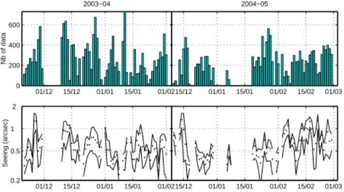
A total amount of 31597 2-minute seeing values have been estimated during the campaigns 2003-2004 and 2004-2005. Thanks to the presence of two observers, several long time se-ries have been made possible, making the monitoring as con-tinuous as possible. As the polar alignment was progressively improved, we could then leave the telescope alone almost 8 hours without losing the star. Figure 4 (top) shows the number of seeing values obtained every day during the two campaigns (maximum possible value is 720). Several periods of lack of measurements were due to bad weather (as in December 2003 where we had 10 successive days of covered sky) or logistics (this is the case in mid-January 2005 where part of the equip-ment was transferred into the Concordia buildings and some work was done to set up the remote control).
Amazingly low seeing values were observed during the first days of the 2003-04 campaign. November 21 corresponds to spring in southern hemisphere; temperature was then close to -50◦C. These temperature conditions are the closest to winter
values we had on the 3 campaigns. First 2 days seeing times series are shown on Fig. 3. Exceptional seeing as low as 0.1′′ has been observed, and we had a continuous period of 10 hours of seeing below 0.6′′. Daily median values are plotted on Fig. 4. Seeing statistics are summarized in Table 2. As mentioned above, all measurements are computed at λ = 500 nm in day-time. Seeing values are in arcsec.
Seeing histograms are displayed on Fig. 5. Scale has been set to logarithmic (base 10) on the seeing axis to emphasize the log-normal distribution of the values. The 50% percentile (the median) is at ǫ = 0.55′′: seeing is then better than 0.55′′half
of the time.
These values are exceptionally good for daytime seeing, when the Sun is present in the sky and heats the surface. It can compare with night-time seeing of the best observatories. Table 3 shows a comparison with other sites.
00:000 03:00 06:00 09:00 0.2 0.4 0.6 0.8 1 1.2 Seeing on 22/11/2003 Local time Transverse Longitudinal 18:000 21:00 00:00 0.2 0.4 0.6 0.8 1 1.2 Seeing on 21/11/2003 Local time Transverse Longitudinal
Fig. 3. First seeing curves obtained during the campaign
2003-2004 on November 21 and 22, 2003. We show here the longi-tudinal (+) and transverse (o) time series.
01/12 15/12 01/01 15/01 01/02 0 200 400 600 2003−04 Nb of data 15/12 01/01 15/01 01/02 15/02 01/03 2004−05 01/12 15/12 01/01 15/01 01/02 0.2 0.5 1 2 Seeing (arcsec) 15/12 01/01 15/01 01/02 15/02 01/03
Fig. 4. Top: Number of seeing data per day. Bottom: points are
daily median seeing values and interval containing 50% of val-ues is delimited by lines. Data collected during the last two summer campaigns. Seeing axis is logarithmic
Table 2. Seeing statistics for the two summer campaigns. These number stand for the DIMM at h = 8.5 m.
Campaign 2003-04 2004-05 Total Number of measurements 17128 14469 31597 Median seeing (′′) 0.54 0.55 0.55 Mean seeing (′′) 0.65 0.67 0.66 Standard deviation (′′) 0.39 0.38 0.39 Max seeing (′′) 5.22 3.33 5.22 Min seeing (′′) 0.10 0.08 0.08 0.15 0.3 0.6 1 2 4 0 2 4 6 8
Seeing (log scale)
Frequency (%) Cumulative Counts (%) 0 20 40 60 80 100
Fig. 5. Histogram (stairs) and cumulative histogram
(continu-ous line) of seeing values for the campaigns 2003-2004 and 2004-2005. Seeing axis is in logarithmic scale.
6 E. Aristidi et al.: Site testing in summer at Dome C, Antarctica
Table 3. Comparison of Dome C daytime seeing with daytime and night-time seeing in other observatories.
Daytime values Night-time values
Site Seeing reference Site Seeing reference
White Sands 2.24 Walters et al. 1979 Paranal 0.66 Sarazin (www.eso.org/∼msarazin)
Sac Peak 1.68 Ricort et al. 1979 Mauna Kea 0.63 Tokovinin et al. 2005
Roque de Muchachos 1.91 Borgnino & Brandt 1982 Roque de Muchachos 0.64 Mu˜noz et al. 1997
Sac Peak 1.16 Brandt et al 1987 Cerro Pachon 0.89 Ziad et al. 2000
Calern 2.5 Irbah et al. 1994 Maidanak 0.69 Eghamberdiev et al. 2000
Fuxian Lake 1.20 Beckers & Zhong 1994 South Pole 1.74 Travouillon et al 2003
Dome C 0.54 this paper Dome C (day) 0.54 this paper
0 10 20 0.3 0.4 0.5 0.6 0.7 0.8 1 seeing (arcsec) Local time 0 5 10 15 20 0.5 0.6 0.7 0.8 1.0 1.2 Seeing (arcsec)
Local time (UT+8) h=3m h=8m
Fig. 6. Left: seeing versus time, averaged over the campaigns
2003-04 and 2004-05. Seeing values, obtained from the DIMM at elevation h = 8 m, have been binned into 30 min intervals. Right: seeing versus time in 2004-2005 for the two DIMMs.
Another interesting result is the behaviour of the seeing with time. Figure 6 has been calculated by binning all see-ing values into 30 min intervals. Best seesee-ing values, like 0.4
′′or better, are generally obtained in mid local afternoon. It is
extremely encouraging for solar imaging at high angular reso-lution. Indeed, a discontinuity of the temperature gradient be-tween 200 and 400 m has often been noted in the middle of the day, and disappears in the evening to be replaced by a standard surface inversion layer of 20 or 30 m (Aristidi et al. 2005). During the afternoon transition, there is a moment with an isothermal temperature profile. The generally excellent seeing obtained during this transition indicates that the contribution of all the rest of the atmosphere is indeed very small. At night with a telescope standing above the ground inversion layer, a really excellent seeing could then be expected almost continuously. The height of this inversion layer is an open question that will be answered after the winterover.
5.1.1. Contribution of the surface layer
During the 2004-05 summer campaign, the presence of two DIMMs observing simultaneously at two different heights (3 m and 8 m over the plateau snow surface) allowed an investi-gation of the contribution of the surface layer to the seeing. Radiosoundings had already shown that the strongest thermal gradients are observed close to the surface (Aristidi et al. 2005) and an important part of the turbulence is expected to be gen-erated in the first tens of meters.
All the telescopes were installed in the first days of December 2004, and the seeing monitoring started for
tele-0 5 10 15 20 0 0.2 0.4 0.6 0.8 1 TER Local time 0 0.5 1 0 50 100 150 200 TER Counts
Fig. 7. Left : surface layer turbulent energy ratio (T ER) as a
function of time. Error bars are the standard deviation of the samples distribution. Right : T ER histogram.
scope 1 (on the ground) and 3 (on the platform) on December 10. Median/mean seeings are 0.55/0.67′′for telescope at 8 m and 0.93/1.03′′for telescope at 3 m (statistics over 15 000
val-ues obtained in December 2004, January and February 2005). There is an important difference which appears to be time-dependent. Figure 6 shows the behaviour of the seeing mea-sured at the two heights, as a function of local time. Both curves exhibit a noticeable minimum in mid-afternoon, though less pronounced for the 3 m curve.
We can describe the surface layer contribution with a tur-bulent energy ratio (TER), following Martin et al. (2000):
T ER = R8m 3m C 2 n(h) dh R∞ 3mC 2 n(h) dh (3)
This T ER gives the ratio of the turbulent energy in the 5 m surface layer to the total turbulent energy (integrated from 3 m to infinity). These integral can be estimated from the seeing through the Fried’s parameter (Roddier 1981). The T ER is then given by
T ER = r0(3m)
−5/3− r
0(8m)−5/3
r0(3m)−5/3 (4)
The T ER was calculated every time the two telescopes were operated simultaneously. Its histogram and time-dependence are shown on Fig. 7. Mean value of 48% indicates that almost half of the ground turbulence is concentrated into the first 5 m above the surface.
Table 4. Isoplanatic angle (θ0) and scintillation index statistics
during the month of January 2004.
θ0(′′) s(%) # of measurements 6368 6368 Mean value 6.8 0.88 Median value 6.8 0.63 standard deviation 2.4 0.90 Min value 0.7 Max value 17.1 0 5 10 15 0 1 2 3 4 5 6 7 θ0 (arcsec) Frequency (%) Cumulative Counts (%) 0 20 40 60 80 100
Fig. 8. Histogram (stairs) and cumulative histogram (line) of
isoplanatic angle values for the campaign 2003-2004.
5.2. Isoplanatic angle and scintillation
More than 6000 values of the isoplanatic angle have been col-lected during the month of January, 2004. Statistics of both θ0 and the scintillation index s summarised in Table 4 show
a median value θ0 = 6.8′′at wavelength λ = 0.5µm, which
is far better than values obtained in any astronomical site (see Table 5 for a comparison). Good values are found also at the South Pole where the atmosphere above the first 220 m is calm (Marks et al. 1999); the isoplanatic angle is indeed more sensi-tive to high altitude turbulence. Winter estimates given by the MASS in the AASTINO station (Lawrence et al. 2004) indi-cates values similar to ours, despite the presence in winter of high-altitude winds of the order of 40 m/s (Aristidi et al. 2005 and references therein).
The histogram and cumulative histogram are shown in Fig. 8, time series on figure 9. The daily median values plot in the top of Fig. 9 shows a small degradation of ¯θ0 between
the beginning and the end of January.
The large value of isoplanatic angle, roughly 3 times larger than in classical sites, is a good news for adaptive optics. This corresponds to a gain of a factor 10 in the field usable to find calibrator stars, and therefore increases the observable piece of sky, as discussed by Coud´e du Foresto (Coud´e du Foresto et al. 2004). Another advantage of a large isoplanatic domain is the uselessness of multi-conjugate adaptive optics for high-resolution wide field imaging (Lawrence 2004).
6. Discussion and conclusion
We have presented the results of optical turbulence measure-ments during two summer campaigns at Dome C. The main
5 10 15 20 25 30 2 4 6 8 10 12 5 10 15 20 25 30 0 200 400 600 N data Date (Jan 2004)
Fig. 9. Isoplanatic angle as a function of day. Top: daily median
values. Error bars corresponds to the 1σ dispersion of the daily values. Bottom: number of data per day.
Table 5. Comparison of Dome C isoplanatic angle with values
observed in other sites.
Site θ0 reference
Paranal 1.91 Ziad et al. 2000
La Silla 1.25 Ziad et al. 2000
Cerro Pachon (Chile) 2.71 Ziad et al. 2000
Maidanak 2.47 Ziad et al. 2000
Oukaimeden (Morocco) 1.58 Ziad et al. 2000
South Pole 3.23 Marks et al. 1999
Dome C 6.8 this paper
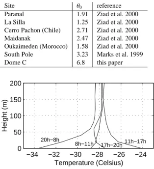
−34 −32 −30 −28 −26 −24 0 50 100 150 200 Temperature (Celsius) Height (m) 20h−8h 11h−17h 8h−11h 17h−20h
Fig. 10. Mean temperature profiles above the ground (from
Aristidi et al. 2005), based on in-situ radiosoundings. On the vertical axis, height is counted from the snow (altitude 3260m). The four curves correspond to measurements performed at four different times of the day
result is the exceptional seeing quality in the daytime, allowing image resolution better than 0.5′′during a few hours every day,
and the large value of the isoplanatic angle, three times larger than Mt Paranal in night-time. Combining this with large peri-ods of clear and coronal sky makes Dome C probably one of the best sites on earth for solar visible and infrared astronomy. We recently published (Aristidi et al. 2005) a study based on balloon-borne meteo radio-sondes launched during 4 sum-mer seasons, allowing us to make statistics on wind speed and temperature profiles in the atmosphere above Dome C. Among the numerous results presented in that paper, we found that the temperature profile exhibit strong gradient in the boundary layer (the first 100 m above the snow). Corresponding curve is shown in Fig. 10. This gradient, positive at midnight(ice is
8 E. Aristidi et al.: Site testing in summer at Dome C, Antarctica 0.1 0.3 0.6 1.0 2.0 0 2 4 6 8 10 Seeing Isoplanatic angle
Fig. 11. Plot of the isoplanatic angle versus seeing (data
col-lected in January 2004).
cooler that the air above) and negative at noon (ice is heated by the Sun radiation), vanishes twice a day: in the morning and near 5pm. Seeing appears indeed to be the best during the af-ternoon near 5pm. The other expected seeing minimum in
the morning has been sometimes observed, especially in the 2003-2004 campaign. But it does not appear in the daily av-eraged curves displayed in Fig. 6 and at this time we have no convincing explanation for that.
This behaviour of the boundary layer temperature profile and of the seeing-versus-time curve suggests that the turbu-lence is dominated by the first tens of meters above the ground. This is the same at the South Pole, where the height of this very turbulent boundary layer is 220 m (Marks et al. 1999). Indeed, another indicator is the correlation between the seeing and the isoplanatic angle. Both result from an integral over the whole atmosphere, but the isoplanatic angle is more sensitive to high turbulent layers (ponderation by h5/3 in the integral definition of θ0(Ziad et al. 2000)). Figure 11 displays a plot of the
isopla-natic angle versus seeing showing no dependence between the two parameters. Quantitative estimations of the surface layer contribution have been made possible in 2004-2005 with the presence of two DIMMs. 50% of the ground seeing is gener-ated in the first 5 m.
Now, the winter measurements are awaited with a lot of excitement, to know how much residual turbulence will exist above this ground layer during the winter night, how thick will be this layer, and how much turbulence will exist below. The last summer campaign was the first one to be immediately fol-lowed by the historical first winter-over, and Agabi has volun-teered to spend one year at Concordia to conduct the observa-tions. Seeing and isoplanatic angle monitoring are in progress. In-situ soundings of the vertical profile of C2nby means of
bal-loon borne microthermal sensors are also at the menu for the winter. They will give access to parameters such as the outer scale and coherence time. Finally a monitoring of C2
n in the
boundary layer is also foreseen, using a ground version of the balloon experiment which takes advantage of the 32 m high American tower.
At the time of writing this paper, the night is getting longer and longer every day and these questions will receive firm an-swers quite soon.
Acknowledgements. We wish to acknowledge both Polar Institutes, IPEV and ENEA for funding the program and for the logistics sup-port. Thanks to all the Concordia staff at Dome C for their friendly and efficient help in setting up the Concordiastro platforms. We are also grateful to our industrial partners “Optique et Vision” and “Astro-Physics” for the technical improvement done on the telescopes and their mounts to make them work in polar conditions. Finally we thank Jean-Michel Clausse and Jean-Louis Dubourg who were present on site during the campaings 2000-2001 and 2001-2002.
References
Aristidi E., Agabi A., Vernin J., Azouit M., Martin F., Ziad A., Fossat E., 2003a, A&A 406, L19
Aristidi E., Agabi A., Vernin J., Azouit M., Martin F., Ziad A., Fossat E., 2003b, Memorie della Societa’ Astronomica Italiana Suppl. vol. 2, p 146
Aristidi E., Agabi A., Azouit M., Fossat E., Vernin J., Travouillon T., Lawrence J., Meyer C., Storey JW., Halter B., Roth W.L., Walden V., 2005, A&A 430, 739
Avila R., Vernin J., Cuevas S., 1998, PASP 110, 1106
Barletti R., Ceppatelli G., Patern`o L., Righini A., Speroni N., A&A 1977, 54, 649
Beckers J.M., Zhong L., 2002, BAAS 34, 735 Borgnino J., Brandt P.N., 1982, JOSO ann. rep., p. 9 Brandt P.N., Mauter H.A., Smartt R., 1987 A&A 188, 163
Coud´e du Foresto V., Swain M., Schneider J., , 2004, EAS eds., proc. of the “Dome C Astronomy-Astrophysics meeting”, Toulouse, June 28 – July 1st, 2004
Ehgamberdiev S., Baijumanov A., Ilyasov S., Sarazin M., Tillayev Y., Tokovinin A., Ziad A., 2000, A&AS 145, 293
Fried D.L., 1966, J. Opt. Soc. Am. 56, 1372
Frieden B.R., 1983, Probability, statistical optics and data testing, Springer, Berlin, p. 248
Heintz W.D., 1960, Veroff. Sternw. Munchen, 5, 100
Irbah A., Laclare F., Borgnino J., Merlin G., 1994, Sol. Phys. 149, 213 Lawrence J., 2004, Appl. Opt. 43, 1435
Lawrence J., Ashley M., Tokovinin A.A., Travouillon T., 2004, Nature 431, 278
Loos G., Hogge C., 1979, Appl. Opt. 18, 2654
Marks R., Vernin J., Azouit M., Manigault J.F., Clevelin C., 1999, A&AS134, 161
Martin H.M., 1987, PASP 99, 1360
Martin F., Conan R., Tokovinin A.A., Ziad A., Trinquet H., Borgnino J., Agabi A., Sarazin M., 2000, A&AS 144, 39
Mu˜noz-Tu˜n`on C., Vernin J., Varela A.M., 1997, A&AS 125, 183
Pourbaix D., Niveder D., McCarthy C. et al. , 2002, A&A 386, 280
Ricort G., Aime C., 1979, A&A 76, 324 Roddier F., 1981, Progress in optics XIX, 281 Sarazin M., Roddier F., 1990, A&A 227, 294 Tokovinin A. 2002, PASP 114, 1156
Tokovinin A., Vernin J., Ziad A., Chun M., 2005, PASP 117, 395 Travouillon T., Ashley M., Burton M., Storey J.W., Conroy P., Hovey
G., Jarnyk M., Sutherland M., Loewenstein R., 2003, A&A 400, 1163
Vernin J, Mu˜noz-Tu˜n`on C, 1995, PASP 107, 265
Walters D.L., Favier D., Hines J.R., 1979 J. Opt. Soc. Am. 69, 828 Ziad A., Conan R., Tokovinin A., Martin F., Borgnino J., 2000,
Appendix A: Error analysis
A.1. Seeing
Statistical error. Variance of image motion is computed from a sample of N ≃ 9000 individual frames: it is then affected by statistical noise due to the finite size of the sample. Assuming statistical independence between the frames, the statistical er-ror on the variance σ2 is given by (Frieden, 1983, Sarazin &
Roddier, 1990) δsσ2 σ2 = r 2 N− 1 (A.1)
that propagates onto the seeing an error contribution δǫ. With
9000 independent frames we haveδsσ2
σ2 = 1.4% and
δsǫ
ǫ = 0.9%.
Frames are not independent at our sampling rate and this is only a lower boundary.
Scale error. Image motion is converted from pixels to arcsec using the factor ξ introduced before. The uncertainty on ξ prop-agates into the differential variances when the conversion from pixels into arcsec is performed. With actual valueδξξ = 0.006
that gives a relative contribution on the differential vari-ancesδpσ2
σ2 = 1.2% and on the seeing
δpǫ
ǫ = 0.7%.
Readout noise Influence of the CCD readout noise on DIMM data is discussed in Tokovinin, 2002. The readout noise is a random independent contribution to the measured flux. It biases the computed differential variances by a term
σ2R = 2R 2 I2 X window x2i j (A.2)
where I is the total stellar flux, R is the readout noise (2.3 ADU for the Pixelfly) and xi j the coordinates of contributing pixels
(the number of illuminated pixels is of the order of 30 after flat fielding and that defines the “window” over which the summa-tion is made). The order of magnitude of this bias in our case is σ2
R ≃ 10−6square pixels. Comparing this value to our standard
differential variances (0.1 to 1 square pixel), we can see that the readout noise bias is extremely small and can be neglected.
Background noise. The sky background is an additive Poisson noise independent from the stellar signal. Therefore its effects on the differential centroid variance is the same as the readout noise: a bias term σ2
B. It can be computed using eq. A.2,
substituting R by B, the background standard deviation (square root of background flux per pixel). The background is a func-tion of time, as shown by Fig. 2; it can attain 30% of the stellar flux when the Sun is at its maximum (typical values in ADU for the highest background are B ≃ 1000). It leads to a bias term σ2B ≃ 10−4square pixels which is still negligible compared to the differential variance values.
A.2. Isoplanatic angle
Background Noise. The presence of a strong background on individual images causes uncertainties and biases on the
esti-mation of the mean stellar intensity ¯I (ensemble average over the image sample), its standard deviation σI and then on the
scintillation index s. As shown on Fig. 2, the background can be as high as 30% of the stellar flux when the Sun is at its max-imum. To perform a bias an SNR estimation, let us introduce the following variables:
– B, the background intensity collected over the NI pixels
il-luminated by the star after threshold application, ¯B and σ2
B
its mean and variance. B is a Poisson random variable, it must verify σB=
√
B, that was well verified on images.
– It the total intensity (background+stellar flux) collected
over the NI pixels.
The stellar flux is given by I = It− B, the measure being It.
The mean ¯I is biased by the term ¯B. This bias is estimated (we
assume stationarity so that the ensemble average ¯B is equal to
the average over one image) and removed as indicated above, but the background fluctuations lead to an error δI on the esti-mation of ¯I equal to δI = σB ≃
√
B.
The variance σ2I is equal to the difference σ2I = σ2It− σ2
B
assuming independence between the stellar flux and the back-ground. The variance estimation we make on images is σ2It, it is then biased by the term σ2
B. However we remarked that this
bias is less than 1% of σ2
Itand decided not to debias the
vari-ances. In addition to this bias, there is an error term δσ2
B due
to the uncertainty of the estimation of σ2
B. Hence the total error
on σ2
I is σ
2
B+ δσ
2
Bif we do not debias the variances.
The scintillation index is the ratio s = σ2
I/ ¯I 2; its error δs can be estimated by δs s = δσ2 I σ2 I + 2δ ¯I ¯I = σ2 B+ δσ 2 B σ2 I + 2σB ¯I (A.3)
Typical values corresponding to the worst case (strongest back-ground at Sun’s maximum elevation) are, in ADU units: σB ≃
400, ¯I ≃ 40000, σI ≃ 5000 and δσ2B ≃ 70000. That gives a
background error contribution δs s = 3%
Readout noise. The readout noise can be considered as a Gaussian random variable with mean r (per pixel) and standard deviation σr = 2.3 ADU (from Pixelfly documentation). As
the star is spread over NIpixels, we will consider the variables
R = NIr (mean over the NI pixels) and its standard deviation
σR =
√
NIσr. The mean value R is automatically removed by
the background substraction. The same reasoning as above can be applied to the readout noise. From Eq. A.3 the contribution
δrs
s of the readout noise is then given by
δrs s ≃ σ2R σ2I + 2 σR ¯I (A.4)
in which we have neglected the term δσ2
R. Taking the same
val-ues than for the background noise we have δps
s ≃ 10−3that is
one order of magnitude below the background noise and can be neglected.