Association and prediction of phenotypic traits from neuroimaging data using a multi-component mixed model excluding the target vertex

HAL Id: hal-03174495

https://hal.archives-ouvertes.fr/hal-03174495

Submitted on 19 Mar 2021

HAL is a multi-disciplinary open access

archive for the deposit and dissemination of

sci-entific research documents, whether they are

pub-lished or not. The documents may come from

teaching and research institutions in France or

abroad, or from public or private research centers.

L’archive ouverte pluridisciplinaire HAL, est

destinée au dépôt et à la diffusion de documents

scientifiques de niveau recherche, publiés ou non,

émanant des établissements d’enseignement et de

recherche français ou étrangers, des laboratoires

publics ou privés.

Association and prediction of phenotypic traits from

neuroimaging data using a multi-component mixed

model excluding the target vertex

Baptiste Couvy-Duchesne, Futao Zhang, Kathryn Kemper, Julia Sidorenko,

Naomi Wray, Peter Visscher, Jian Yang, Olivier Colliot

To cite this version:

Baptiste Couvy-Duchesne, Futao Zhang, Kathryn Kemper, Julia Sidorenko, Naomi Wray, et al..

As-sociation and prediction of phenotypic traits from neuroimaging data using a multi-component mixed

model excluding the target vertex. SPIE Medical Imaging 2021, Feb 2021, Virtual, United States.

pp.10, �10.1117/12.2581022�. �hal-03174495�

Association and prediction of phenotypic traits from neuroimaging

data using a multi-component mixed model excluding the target vertex

Baptiste Couvy-Duchesne

, Futao Zhang

, Kathryn E. Kemper

, Julia Sidorenko

, Naomi R.

Wray

*, Peter M. Visscher

*, Jian Yang

*, Olivier Colliot

*

a

_{:Institute for Molecular Bioscience, the University of Queensland, St Lucia, QLD, Australia;}

_{:Institute for Advanced Research, Wenzhou Medical University, Wenzhou, Zhejiang 325027,}

China;

:Paris Brain Institute (ICM), Inserm U1127, CNRS UMR 7225, Sorbonne University, Inria,

Aramis project-team, F-75013, Paris, France; * these authors contributed equally.

1. INTRODUCTION

The increasing sample sizes from neuroimaging studies should allow detection of image measures are associated with phenotypic traits with smaller effect sizes, which will advance progress in the mapping of the brain regions associated with traits and diseases [1]. The UK Biobank (UKB) is one of the best example of this new generation of samples [2]. Multimodal Brain MRI collection is currently ongoing, with tens of thousands of individuals already imaged out of a target of 100,000 [2]. The large sample size, together with the breadth of phenotyping (incl. self-reports, in lab assessments, prescription and medical history), should allow new insights into the factors contributing to brain differences between older adults.

The current approach to map brain regions associated with a trait of interest, consists in mass-univariate analyses, where one tests the association between the trait of interest and each vertex/voxel in turn. The state of the art approach, implemented in most neuroimaging pipelines, uses a general linear model (GLM), which controls for covariates (often age, sex and head size).

The structure of correlation present in neuroimaging data (here, cortical and subcortical thickness and surface area) introduces additional complexity in association testing. It implies that association at a vertex also tags association from other vertices (with which it is correlated) causing an inflation of false positives rate. We previously demonstrated this concern [3], and showed that state of the art GLM could result in more than 60% of the significant clusters being false positives. Instead, we proposed a Linear Mixed Model approach (LMM), which allows controlling for all vertices by fitting them as random effects in the model. We found that LMMs can limit the contamination of signal due to correlation between features, leading to increased mapping precision (smaller true positive clusters) and a greatly reduced probability to observe false positive clusters [3].

However, LMMs exhibited false positive clusters in about 16% of the time, which is still above the 5% mark that one usually considers acceptable. In addition, LMMs may suffer from a slightly reduced power compared to GLM, though it is difficult to compare power when the methods exhibit such different rates of false positive associations [3].

In the present paper, we attempted to overcome these problems, by considering a more complex mixed model, called MOMENT (Multi-cOmponent Mixed model ExcludiNg the Target), which has been used to solve similar issues in omics association studies [4]. MOMENT excludes the target vertex (vertex being tested and those locally correlated with it) from the random effects which avoids the reduction of power seen in LMMs due to “double fitting” [5]. In addition, MOMENT partitions the vertices into two groups (null and associated vertices) in a data driven manner. This allows relaxing the hypothesis of a single normal distribution of effect sizes in the random effect, for example allowing for strongly associated vertices. We evaluated the performance of MOMENT using phenotypes simulated from real MRI images. This allows comparison of false positive and true positive rates of the competing methods.

2. DATA

Our final sample for the analyses comprised 8,662 volunteers imaged as part of the UK Biobank imaging study [2]. Participants were 62.5 years old on average (SD=7.5, range 44-79), and 52.4% were females. The individuals in our

sample had i) a T1w image labelled “usable” by the biobank; ii) a complete FreeSurfer 6.0 + ENIGMA-shape processing; iii) non-outlying brain as per our automated quality control. All aspects of image processing and quality control have been described previously [3, 6].

We used an additional 4,160 UKB participants (63.1 years old, SD=7.46, range 46.1-80.3, with 52.1% of females) as an independent sample to evaluate prediction accuracy achieved from significant grey-matter regions. The data from these participants was from the second release of data from the UKB and were processed in the same way.

2.2. MRI image processing

Our brain MRI processing relied on T1w and T2 FLAIR images (T1w only when T2 was not usable, <3% of participants [3, 6]). We performed the FreeSurfer 6.0 “recon-all” pipeline to extract fine grained cortical thickness and surface area (“fsaverage” mesh, ~600,000 measurements per individual). In addition, we used the ENIGMA-Shape package [7, 8] to extract subcortical thickness and surface area of seven subcortical structures (~50,000 additional measurements). We did not smooth the cortical grey-matter maps, because we previously observed that smoothing reduced the amount of information contained in the processed images, for a wide range of UKB traits [6].

3. METHODOLOGY

We simulated phenotypes from the processed MRI images, varying the number of associated brain regions and the strength of these associations. In the first scenario, we simulated phenotypes associated with 10 grey-matter regions, each accounting for 2% of the trait variance (i.e. brain-morphometricity of R2=0.2 in total). Then, we simulated traits associated with 100 grey-matter regions each accounting for 0.5% of the variance (morphometricity of R2_{=0.5). Finally,}

we used 1000 associated brain regions, each accounting for 0.04% of the trait variance (morphometricity of R2_{=0.4). We}

selected the associated brain regions at random, and simulated 100 phenotypes for each scenario (see [3] for more details).

3.2. Mass-univariate association models

The different models may be written as:

GLM controlling for age, sex and ICV: phenotype = u + b1*age + b2*sex + b3*ICV + b*vertex + 𝜀 (1)

LMM – (global BRM): phenotype = u + b*vertex + 𝛽 + 𝜀 ; with 𝛽 ~ N(0, BRM * 𝜎2_{) (2)}

𝛽 is a vector of random effects, which accounts for the effects of all vertices Z (Nxp matrix, p>N)

[3]

MOMENT: phenotype = u + b*vertex + 𝛽0 + 𝛽1 + 𝜀 (3)

𝛽0 ~ N(0, BRM0 * 𝜎02) the random effect corresponding to “non-associated” vertices. 𝛽1 ~ N(0, BRM1 * 𝜎12) the

random effect of “associated” vertices (excluding target and correlated region).

We used an efficient approximation of the MOMENT model, in order to avoid re-estimating the BRMs and the variance components (𝜎02 and 𝜎12) for each vertex tested, which requires a huge computational cost [5, 9]. First, we selected the

vertices that did not reach significance (after Bonferroni correction) using a GLM, to be fitted in 𝛽0. For each “target

vertex” not included in 𝛽0, we adapted 𝛽1 to include vertices not in 𝛽0 with the exception of the target vertex and its

“flanking region” (vertices strongly correlated with target vertex). This approach prevents from a loss of power because of fitting the vertex of interest twice in the model (once as fixed and again as a random effect) [5, 9]. Our approximated MOMENT is computationally efficient if the number of vertices included in 𝛽1 remains limited. However, MOMENT

requires to define a “flanking region”, for which we used a cut-off based on the coefficient of determination (R2 _or

correlation squared) with the target vertex. Thus, the “flanking region” should contain the surrounding vertices in strong correlation with the target but could also include distal vertices. In the following, we considered eight different R2

We tested the association with each vertex using a

χ

correction. We used the OSCA software [4] for phenotype simulation and mass-univariate analyses, and R (3.6.2) [10] for plots and interpretation of the associations.

3.3. Comparison of the model performances

As in a previous study[3], we first quantified the inflation of test-statistics observed on non-associated (null) vertices. We used the inflation factor, which is the ratio of observed/expected median test statistic of the null vertices. Next, we measured statistical power using the True Positive Rate (proportion of truly associated vertices reaching significance, after Bonferroni correction). Regarding false positives, we reported the Family-Wise Error Rate (FWER, proportion of replicates with at least one false positive vertex), the cluster FWER (proportion of replicates with at least one positive cluster) and the cluster False Discovery Rate (FDR) defined as the proportion of significant clusters that are false positives. We expect the FWER to be greater than 5% in presence of strong local correlation between neighboring vertices, which leads to clusters of associations comprising several contiguous vertices. The cluster FWER is thus our main metric of false positive, as it quantifies the probability of observing an association in a non-associated brain region. We further reported mapping precision as median size of the true positive clusters, and prediction accuracy achieved from significant grey-matter regions.

4. RESULTS

First, we studied the distribution of test-statistics across null vertices. We found that using GLMs resulted in an inflation of the null test statistics, while using the LMM or MOMENT appropriately controlled the inflation (Figure 1). As for statistical power (measured using the true positive rate), we found MOMENT to be as powerful as the GLM, while the LMM “global BRM” exhibited a slight reduction in number of true associations reaching significance (most notable for scenario 2, see Figure 1).

For scenarios 2 and 3, MOMENT failed to reduce the probability of detecting a false positive vertex (FWER) or cluster (cluster FWER, Figure 1), compared to the LMM. The proportion of false positive clusters (cluster FDR) was also greater using MOMENT than when using LMM, even if it was much lower than that seen using GLM. Of note, MOMENT did outperform the LMM in the simplest scenario (10 associated vertices), which may be due to the presence of large(r) associations, though we cannot rule out it may be influenced by the location of those associations in the brain.

The cut-off value used to define the flanking region in MOMENT, had little effect on the metrics presented in

Figure 1. The most notable effect was observed on cluster FDR in scenario 3, where lowering the cut-off led to an

increased proportion of false positive clusters (Figure 1).

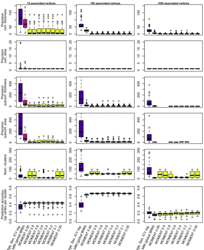
Beyond power and false positives, using MOMENT offered an increased mapping precision, which superseded the best performing LMM, within each type of measurement (Figure 2). Finally, we evaluated how the differences in power, false positives and estimates could impact precision accuracy, which we use as a global metric of model performance. We found that MOMENT tended to yield the best prediction accuracy, on par or greater than the other models (Figure 2). We also observed that the number of significant clusters (hence number of vertices included in the predictor) was lower, and less variable, when using R2 values between 0.2 and 0.8 to define the flanking region. This suggests that values in this range should be preferred in order to be conservative, even though the greater number of significant clusters does not seem to worsen the cluster FWER and FDR.

Figure 1: Test inflation, statistical power and false positives of the different models

Here, we compare the performances of GLM, LMM and MOMENT in three different simulation scenarios (columns). Depending on the metric, we report the distribution (boxplots) or estimates and SE (point plots) over the 100 phenotypes simulated. The numbers following the MOMENT label correspond to the R2 _{used to define the flanking region.}

Figure 2: Mapping precision and prediction accuracy from significant clusters using the different models

Here, we compare the performances of GLM, LMM and MOMENT in three different simulation scenarios (columns). We report the metrics distribution (boxplots) over the 100 phenotypes simulated. The numbers following the MOMENT label correspond to the R2 _{used to define the flanking region.}

5. CONCLUSION

We evaluated MOMENT, a multi-component mixed model which has been proposed for MWAS, in order to minimize the probability of false positives. We used MOMENT on traits simulated from grey-matter vertex-wise data and compared its performance against that of traditional GLM and more parsimonious LMM.

In terms of association, we found somewhat mixed results for MOMENT. On the plus side, MOMENT did not show any inflation of the null test statistic, which is a characteristic of mixed models [5]. MOMENT also had the highest true positive rate, on par with that of GLM, and greater than that of LMM (Figure 1). Finally, MOMENT maximized mapping precision, out of all models considered, with a median true positive cluster size of less than 30 vertices (Figure

2). However, MOMENT performed worse than LMM at controlling the probability of false positive clusters and their

proportion (in particular for simulations with >100 associated brain regions, Figure 1). For the simplest phenotypes (10 associated brain regions), MOMENT did seem to minimize the cluster FWER and cluster FDR, which may be due to the presence of large(r) brain-trait associations. Indeed, MOMENT allows for large(r) associations to be present, which is the main advantage of the multi-component approach.

For prediction, MOMENT maximized the out of sample prediction, from significant clusters, suggesting that the power increase could compensate the worsening of false positive rate. The different hyper-parameters we evaluated for MOMENT had little effect on the results and model performances, even if some of the extreme values considered (>0.8 and <0.2) may lead to more variable results (Figure 2). The OSCA default definition of the flanking region (R2_{>0.6) appears appropriate for analyzing the grey-matter data.}

Our results contrast with those reported for MWAS, where MOMENT was showed to minimize false positive rate but to result in a lower power than LMM [4]. More work is needed to identify the factors that influence the performances of MOMENT. Such factors might include the presence of large associations (see scenario 1), more generally the pattern of correlation between features (including the correlation induced by confounders), or the definition of the flanking region. Indeed, unlike in the original MOMENT paper [4], we defined the flanking regions based on the R2_{, rather than on the physical distance between features. This is because distance is difficult to define within a folded}

mesh, and even more between meshes.

In conclusion, we evaluated a new model for mass-univariate association studies of grey-matter structure. In association studies, its mixed performances may limit its use for situations where discoverability is the main objective of the study. For conservative inference, our data suggest that LMM should be preferred, even though MOMENT may be more appropriate in presence of large effect sizes. On the other hand, MOMENT led to the highest out-of-sample prediction accuracy which suggests that it could be the method of choice in this setting.

REFERENCES

[1]

[2] K. L. Miller, F. Alfaro-Almagro, N. K. Bangerter et al., “Multimodal population brain imaging in the UK Biobank prospective epidemiological study,” Nat Neurosci, 19(11), 1523-1536 (2016).

[3] B. Couvy-Duchesne, F. Zhang, K. E. Kemper et al., "Linear Mixed Models Minimise False Positive Rate and Enhance Precision of Mass Univariate Vertex-Wise Analyses of Grey-Matter." 404-407.

[4] F. Zhang, W. Chen, Z. Zhu et al., “OSCA: a tool for omic-data-based complex trait analysis,” Genome Biol, 20(1), 107 (2019).

[5] J. Yang, N. A. Zaitlen, M. E. Goddard et al., “Advantages and pitfalls in the application of mixed-model association methods,” Nat Genet, 46(2), 100-6 (2014).

[6] B. Couvy-Duchesne, L. T. Strike, F. Zhang et al., “A unified framework for association and prediction from vertex-wise grey-matter structure,” Human Brain Mapping, n/a(n/a), (2020).

[7] B. A. Gutman, S. K. Madsen, A. W. Toga et al., [A Family of Fast Spherical Registration Algorithms for Cortical Shapes] Springer International Publishing, Cham(2013).

[8] B. A. Gutman, Y. L. Wang, P. Rajagopalan et al., “Shape Matching with Medial Curves and 1-D Group-Wise Registration,” 2012 9th Ieee International Symposium on Biomedical Imaging (Isbi), 716-719 (2012).

[9] J. Listgarten, C. Lippert, C. M. Kadie et al., “Improved linear mixed models for genome-wide association studies,” Nat Methods, 9(6), 525-6 (2012).

[10] R Development Core Team, [R: A Language and Environment for Statistical Computing] R Foundation for Statistical Computing, Vienna, Austria(2012).