Developing environmental indices using fuzzy numbers ordered weighted averaging (FN-OWA) operators

Publisher’s version / Version de l'éditeur:

Stochastic Environmental Research & Risk Assessment, 22, January 1, pp. 495-505, 2008-01-01

READ THESE TERMS AND CONDITIONS CAREFULLY BEFORE USING THIS WEBSITE. https://nrc-publications.canada.ca/eng/copyright

Vous avez des questions? Nous pouvons vous aider. Pour communiquer directement avec un auteur, consultez la

première page de la revue dans laquelle son article a été publié afin de trouver ses coordonnées. Si vous n’arrivez pas à les repérer, communiquez avec nous à PublicationsArchive-ArchivesPublications@nrc-cnrc.gc.ca.

Questions? Contact the NRC Publications Archive team at

PublicationsArchive-ArchivesPublications@nrc-cnrc.gc.ca. If you wish to email the authors directly, please see the first page of the publication for their contact information.

NRC Publications Archive

Archives des publications du CNRC

This publication could be one of several versions: author’s original, accepted manuscript or the publisher’s version. / La version de cette publication peut être l’une des suivantes : la version prépublication de l’auteur, la version acceptée du manuscrit ou la version de l’éditeur.

For the publisher’s version, please access the DOI link below./ Pour consulter la version de l’éditeur, utilisez le lien DOI ci-dessous.

https://doi.org/10.1007/s00477-007-0151-0

Access and use of this website and the material on it are subject to the Terms and Conditions set forth at Developing environmental indices using fuzzy numbers ordered weighted averaging (FN-OWA) operators

Sadiq, R.; Tesfamariam, S.

https://publications-cnrc.canada.ca/fra/droits

L’accès à ce site Web et l’utilisation de son contenu sont assujettis aux conditions présentées dans le site LISEZ CES CONDITIONS ATTENTIVEMENT AVANT D’UTILISER CE SITE WEB.

NRC Publications Record / Notice d'Archives des publications de CNRC: https://nrc-publications.canada.ca/eng/view/object/?id=c61522a0-966e-432a-9d78-3c4ed96aa4ca https://publications-cnrc.canada.ca/fra/voir/objet/?id=c61522a0-966e-432a-9d78-3c4ed96aa4ca

http://irc.nrc-cnrc.gc.ca

D e v e l o p i n g e n v i r o n m e n t a l i n d i c e s u s i n g f u z z y

n u m b e r s o r d e r e d w e i g h t e d a v e r a g i n g ( F N

-O W A ) o p e r a t o r s

N R C C - 5 0 4 4 7

S a d i q , R . ; T e s f a m a r i a m , S .

A version of this document is published in / Une version de ce document se trouve dans: Stochastic Environmental Research & Risk Assessment, v. 22, no. 1, Jan. 2008, pp. 494-505 doi: 10.1007/s00477-007-0151-0

The material in this document is covered by the provisions of the Copyright Act, by Canadian laws, policies, regulations and international agreements. Such provisions serve to identify the information source and, in specific instances, to prohibit reproduction of materials without written permission. For more information visit http://laws.justice.gc.ca/en/showtdm/cs/C-42

Les renseignements dans ce document sont protégés par la Loi sur le droit d'auteur, par les lois, les politiques et les règlements du Canada et des accords internationaux. Ces dispositions permettent d'identifier la source de l'information et, dans certains cas, d'interdire la copie de documents sans permission écrite. Pour obtenir de plus amples renseignements : http://lois.justice.gc.ca/fr/showtdm/cs/C-42

Developing Environmental Indices using Fuzzy Numbers Ordered

Weighted Averaging (FN-OWA) Operators

Rehan Sadiq1 and Solomon Tesfamariam

Urban Infrastructure Program, Institute for Research in Construction, National Research Council Canada (NRC-IRC), Ottawa, ON, Canada K1A 0R6

Abstract: Environmental indices (EI) are common communication tool used to describe the overall status of environmental systems (e.g. air, water, soil). Development of EI entails the use of

mathematical operators to aggregate various non-commensurate input parameters in a logical manner. Ordered weighted averaging (OWA) operator is a general mean type operator that provides flexibility in the aggregation process such that the aggregated value is bounded between minimum and maximum values of the input parameters. This flexibility of OWA operator is realized through the concept of orness, which is a surrogate for decision maker’s attitude.

For the development of environmental indices, the type of input parameters also affects the choice of aggregation operators. If the input parameters are linguistic or fuzzy, the aggregation through OWA operators is not possible, and the use of fuzzy arithmetic is warranted. To develop EI, the concept of FN-OWA (fuzzy number OWA) operators is explored to handle the situations when one ore more input parameter has fuzzy (or linguistic) values. The proposed approach is demonstrated using data provided in an earlier study by Swamee and Tyagi (2000) for establishing water quality indices. Multiple hypothetical scenarios are also generated to highlight the utility and the sensitivity of the proposed approach.

Keywords: Environmental indices, fuzzy number ordered weight averaging (FN-OWA), similarity measures, and fuzzy arithmetic.

INTRODUCTION

Environmental indices (EI) are used as a communication tool to describe overall status of the

environmental systems (including land, air, water etc.). EI can be used to summarize a large numbers of environmental indicators in a meaningful way (Ott 1978). EI can also help in selecting

appropriate decision actions for the improvement of environmental quality by considering various conflicting factors. Significant literature is available on the use of statistical and mathematical aggregation methods to develop indices for air, water and sediment quality. These data aggregation methods generally include logical operators (and, or), averaging or compromising operators

(arithmetic average, weighted average, geometric mean, weighted product), and other methods such as simple addition, root sum power, root sum-square, and multiplicative forms (Somlikova and Wachowiak 2001; Silvert 2000; Ott 1978). Swamee and Tyagi (2000) have discussed the advantages and shortcomings of different aggregation techniques to develop EI. Detailed discussions on the selection of appropriate aggregation operators can be found in Klir and Yuan (1995), and Smolikova and Wachowiak (2001).

Recognition of two potential pitfalls, namely exaggeration and eclipsing is very important in the aggregation process (Ott 1978). Exaggeration is a case when all environmental quality indicators individually posses lower value (i.e., acceptable range), yet the EI comes out unacceptably high. Eclipsing is the converse phenomenon, where one or more of the environmental quality indicators are of relatively high value (i.e., in an unacceptable range), yet the estimated EI comes out as

unacceptably low. These phenomena are typically affected by the method of aggregation, thus the

challenge is to determine the best aggregation method that can simultaneously reduce both

exaggeration and eclipsing.

To maintain ‘acceptable’ environmental quality, the guidelines and standards for certain

environmental indicators (including physico-chemical, microbiological, aesthetic) are established and consequently linked to the possible adverse health impacts on humans and ecological entities. Therefore, numerous environmental indicators can be linked to some sort of crisp ‘acceptability’ measure. Silvert (2000) argued that the concept of ‘acceptability’ itself is fuzzy because we may measure ‘health’ effects more accurately than we can evaluate their ‘importance’. Recently, a large number of water and air quality indices have been reported in the literature using fuzzy synthetic evaluation (including techniques like fuzzy classification, fuzzy similarity method and fuzzy

comprehensive assessment) and fuzzy rule-based modelling (Sadiq et al. 2007; Sadiq and Rodriguez 2004; Lu and Lo 2002;Chang et al. 2001; Lu et al. 1999; Tao and Xinmiao 1998).

To simultaneously reduce both exaggeration and eclipsing, in this paper ordered weighted

averaging (OWA) operators (Yager 1988) is used. The OWA operator provides flexible aggregation

that is bounded between the minimum and maximum operators. The OWA weight generation incorporates decision maker’s attitude or tolerance, which can also be related to perceived

importance of the environmental system under study. There are numerous reported applications of OWA operators in the disciplines of Civil and Environmental Engineering (Sadiq and Tesfamariam 2007; Makropoulos and Butler 2006; Smith 2006). However, to incorporate the fuzzy ‘acceptability’ measures, a fuzzy number OWA (FN-OWA) is further proposed so that it can handle fuzzy or linguistic values and deal with uncertainty by specifying ‘acceptable’ environmental quality. The outline of the paper is as following. Section 2 will explore the concept of fuzzy number OWA and a primer on fuzzy arithmetic operations. Section 3 shows application of the proposed method using an example from Swamee and Tyagi (2000) for establishing water quality indices. Sections 4 and 5 provide discussions and conclusions, respectively.

FUZZY NUMBER OWA (FN-OWA)

The OWA operators are used for aggregating crisp numbers (or fuzzy singletons). In this paper, the use of OWA operator is extended to fuzzy numbers, which is also called FN-OWA operator.

Recently, many attempts have been made in this direction, which include Ahn (2006); and Chang et

al. (2006); Chen and Chen (2005, 2003a); Xu and Da (2002); Carlsson and Fullér (2000); Mitchell

and Estrakh (1998). To help understand the concept of FN-OWA, first fuzzy arithmetic and later OWA operators are discussed.

Fuzzy arithmetic

Fuzzy arithmetic is a generalized form of interval analysis, which is used to address uncertain and/or vague information. A fuzzy number describes the relationship between an uncertain quantity x and a membership function μx, which ranges between 0 and 1. A fuzzy set is an extension of the classical

set theory (in which x is either a member of set A or not) in that an x can be a member of set with a certain membership function μ

A

bell, triangular, trapezoidal, Gaussian). In this paper, trapezoidal fuzzy numbers (ZFN) are used for the analysis. Trapezoidal fuzzy number can be represented by four vertices (a, b, c, d) on the

universe of discourse (scale X on which a criterion is defined), representing the minimum, most likely

interval, and maximum values, respectively. Triangular fuzzy number (TFN) is a special case of

ZFN, where b = c.

One important feature of fuzzy numbers (sets) is the concept of α-cuts. The α-cut of a fuzzy set is a crisp set (interval) A

A

α

that contains all the elements of the universal set X whose membership

grades in are greater than or equal to the specified value of an α, i.e., . Fuzzy

arithmetic is performed based on two properties (Klir and Yuan 1995): a) each fuzzy number, can fully and uniquely be represented by its α-cut; and b) α-cuts of each fuzzy number are closed intervals of real numbers for all . Hence, once the interval is defined, traditional interval analysis can be used (Ferson and Hajagos 2004). Some commonly used interval analysis operations are listed in Table 1, which can be used to carry out fuzzy arithmetic at various predefined α-cut levels, e.g., (0, 0.1, 0.2,…, 1). A Aα =

{

x|μ_x ≥α

}

] 1 , 0 ( ∈ α

Ordered weighted averaging (OWA) operators

Most multi-criteria decision analysis problems neither require strict “anding” (minimum) nor require strict “oring” of the s-norm (maximum). For example, these two extremes for mutually exclusive probabilities correspond to multiplication (and-gate) and summation (or-gate) of a fault tree analysis. To generalize this idea, Yager (1988) introduced a new family of aggregation techniques called the ordered weighted averaging (OWA) operators, which form a general mean type operator. The OWA operator provides a flexibility to utilize the range of “anding” (or “oring”) to include the attitude of a decision maker in the aggregation process. The OWA operation involves three steps – (1) reorder the input arguments, (2) determine weights associated with the OWA operators, and (3) aggregate.

The OWA operator of dimension n is a mapping of , which has an associated weighting

vector , where R Rn → n T n w w w , , , ) (

w= _{1 2} L w_j∈[0,1] and . Hence, for a given n-input

parameters vector ( ∑nj=1wj =1 n x x x ,~ ,...,~ ~ 2

( )

= =∑ = n j j j n w y x x x OWA EI Index tal Environmen 1 2 1,~ ,...,~ ) ~ ~ ( ₍₁₎ where yj ~ _{is the j}th

largest number in the vector (x~₁,x~₂,...,x~_n), and ~y₁≥~y₂ ≥...≥~y_n. Therefore, the weights w_j of OWA are not associated with any particular value x~ , rather they are associated to _j

the ‘ordinal’ position of ~ . The linear form of OWA equation aggregates n-input parameters vector y_j

(~x₁,x~₂,...,~x_n), and provides a nonlinear solution (Yager and Filev 1994).

The range between minimum and maximum values can be determined through the concept of orness (β), which is defined as (Yager 1988):

∑ − − = = n i i i n w n 1 ) ( 1 1 β , and β∈[0,1] (2)

The orness characterizes the degree to which the aggregation is like an or operator. The β = 0, refers to a scenario that vector w becomes (0, 0, …, 1), i.e., an input parameter with the minimum value in the n-input parameters vector (x~₁,~x₂,...,x~_n) is assigned the full weight, which implies that

the OWA becomes a minimum operator. When β = 1, the OWA vector w becomes (1, 0, …, 0), i.e., an input parameter with a maximum value in the n-input parameters vector (x~₁,~x₂,...,x~_n) is assigned

complete weight, which implies that the OWA collapses to maximum operator. Similarly, when β = 0.5, the OWA vector w becomes (1/n, 1/n, …, 1/n), i.e., an arithmetic mean of the input parameter vector (x~₁,x~₂,...,~x_n).

Determining OWA weights

One of the major challenges in OWA method is to generate weights. Different methods of OWA weights generation are reported in the literature. A class of function used to generate OWA weights, called regularly increasing monotone (RIM) quantifier, was first proposed by Yager (1988). The RIM functions are bounded by two linguistic quantifiers “there exists” (OR) and “for all”,

(AND). Thus, for any RIM quantifier , the limit holds true (Yager

and Filev 1994). The OWA weights can be generated using a RIM quantifier as follows: ) (r Q∗ ) (r Q_∗ Q(r) Q_∗(r)≤Q(r)≤Q∗(r) ) (r Q

⎟ ⎠ ⎞ ⎜ ⎝ ⎛ − − ⎟ ⎠ ⎞ ⎜ ⎝ ⎛ = n i Q n i Q w_i 1 i=1,2,...,n (3)

Yager (1996) defined a parameterized class of fuzzy subsets, which provide families of RIM quantifiers that change continuously between Q_∗(r) and Q∗(r):

δ

r r

Q( )= r ≥0 (4)

(1) For δ =1; Q(r) = r (a linear function) called the unitor quantifier (2) Forδ →∞; Q_∗(r), the universal quantifier (and-type)

(3) Forδ →0; , the existential quantifier (or-type) Q∗(r) Therefore Equation (3) can be generalized as

δ δ ⎟ ⎠ ⎞ ⎜ ⎝ ⎛ − − ⎟ ⎠ ⎞ ⎜ ⎝ ⎛ = n i n i w_i 1 i=1,2,...,n (5)

where δ is a degree of a polynomial function. For δ = 1, the RIM function is like a uniform distribution, i.e., equal weights are assigned to ~x₁,x~₂,...,~x_n and becomes an arithmetic mean, i.e., wi

= 1/n. For > 1, the RIM function leans towards right, i.e., “and-type” operators manifesting negatively skewed OWA weight distributions. Similarly, for

δ

δ < 1, the RIM function leans towards left, i.e., “or-type” operators manifesting positively skewed OWA weight distributions. Discussion on the selection of an appropriate value is provided in later sections. δ

Reordering (ranking) of fuzzy numbers using defuzzification

The OWA operators defined in previous sections can be transformed into FN-OWA, for the n-fuzzy input parameters, i.e., described as a set of fuzzy numbers (~x₁,~x₂,...,x~_n). Three steps required for

OWA operators are also valid for FN-OWA operators. The only difference is the reordering and ranking of an n-fuzzy input parameters vector (x~₁,x~₂,...,x~_n), which is not trivial.

Defuzzification is an important step in fuzzy modelling and fuzzy multi-criteria decision-making. The defuzzification entails converting the fuzzy value into a crisp value, and determining the ordinal

positions of n-fuzzy input parameters vector (~x₁,~x₂,...,~x_n). Many defuzzification techniques are

available (Chen and Hwang 1992), but the common defuzzification methods include centre of area, first of maximums, last of maximums, and middle of maximums (MoM).

Different defuzzification techniques extract different levels of information, consequently are prone to rank reversal (Prodanovic and Simonovic 2002). In this paper, the MoM is proposed for

defuzzification to determine the ordering of fuzzy n-input parameters in a vector (x~₁,x~₂,...,~x_n). The

MoM method uses the arithmetic mean of the maximum memberships in a given fuzzy set. For example, in case of ZFN, it is the middle (mean) value xO_j of the most likely interval.

Interpreting FN-OWA results for decision-making

The estimated EI should be assigned a linguistic or a qualitative scale to guide informed decision-making. These linguistic constants or qualitative scales can also be defined as trapezoidal fuzzy numbers ZFNs (ak, bk, ck, dk). We proposed five linguistic constants (k = 1, 2,…,5) over the universe

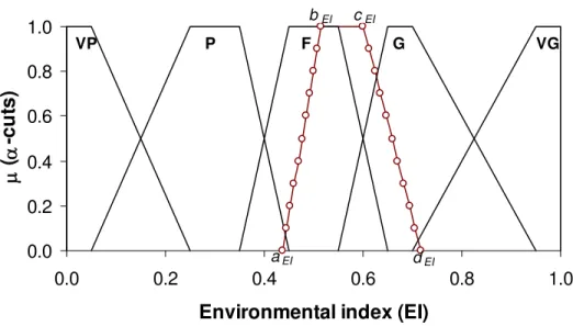
of discourse (a quantitative scale on which environmental indices are defined), namely, very poor (VP), poor (P), fair (F), good (G) to very good (VG) (Table 2). The estimated EI and linguistic constants are superimposed over the universe of discourse. Based on the maximum similarity between a linguistic constant and the estimated EI, a linguistic constant is assigned which can be related to a specific decision action. Smaller the distance between the estimated EI and a particular linguistic constant, higher will be the similarity measure and vice versa.

Various distance measures (DM) are proposed in the literature to compute similarity between two fuzzy sets, e.g. Hamming, Euclidean and Chebyshev (chessboard) distances. Each distance measure has its advantages and shortcomings. Chen (1996) proposed a simple technique to estimate similarity measure (SM) between two ‘normal’ ZFNs. Chen and Chen (2003b) generalized the Chen’s (1996) method by extending to subnormal fuzzy numbers. In this paper, we modified Chen’s (1996) method and used weighted mean instead of arithmetic mean. Larger importance weights ( ) are assigned to most likely values and smaller weights are assigned to minimum and maximum values. Therefore, a similarity between an estimated EI (a

SM l

w

EI, bEI, cEI, dEI), and a given linguistic constant k (ak, bk, ck,

[

]

[

5 1

]

4 3 2 1 1 1 ) , ( = = − − + − + − + − − = − = k k k EI SM k EI SM k EI SM k EI SM a d d d w c c w b b w a a w DM k EI SM (6)

where ( } ) are importance weights, which are assigned values of ,

, , and . Chen’s (1996) method becomes a special case, where equal

importance weights are specified, . The factor in the denominator is

introduced to normalize so that DM and SM∈ [0, 1]. In our case, the denominator is 1 (a maximum possible value EI can attain).

SM l w l={1,2,3,4 w₁SM =0.2 3 . 0 2 = SM w w₃SM =0.3 w₄SM =0.2 25 . 0 4 3 2 1 = = = = SM SM SM SM w w w w An illustrative example

A step-by-step procedure of implementing FN-OWA is illustrated using an example of a 3 input parameters vector. The input parameters in a vector (~x₁,~x₂,~x₃) are assumed trapezoidal fuzzy

numbers defined by four vertices (ai, bi, ci, di). Now further assume that each entry in a vector

(~x₁,~x₂,~x₃) has following values:

1 ~_{x = (0.15, 0.15, 0.20, 0.50);} 2 ~_{x = (0.40, 0.45, 0.50, 0.55); and} 3 ~_{x = (0.50, 0.60, 0.70, 0.80).}

Step 1) Reorder the input parameters

First perform defuzzification using MoM method

O x₁ = (0.15 + 0.20)/2 = 0.175 O x2 = (0.45 + 0.50)/2 = 0.475; and O x₃ = (0.60 + 0.70)/2 = 0.650

1 ~ y = (0.50, 0.60, 0.70, 0.80) 2 ~ y = (0.40, 0.45, 0.50, 0.55); and 3 ~ y = (0.15, 0.15, 0.20, 0.50);

Step 2) Determine the OWA weights (n = 3) using RIM function (let δ = 1/3)

For δ = 1/3, the OWA weights (Equation 5) and orness (Equation 2) are calculated to be

w = (0.69, 0.18, 0.13) and orness β = 0.78.

Step 3) Aggregate using FN-OWA and interpret results

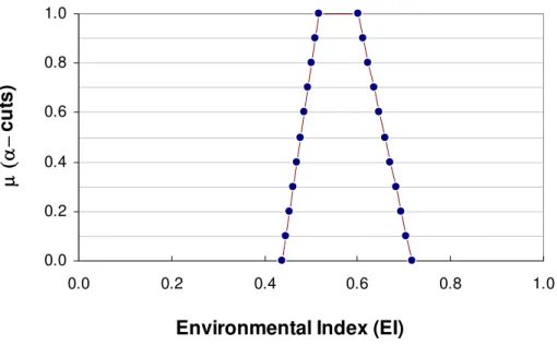
Aggregation process is carried out using interval analysis (Table 1) at predefined α-cut levels. Corresponding to each α-cut, the interval values of the EI are calculated. Results of the interval analysis are as follows:

α-cut 1 ~ y 2 ~_y 3 ~_y *EI 0.0 [0.50, 0.80] [0.40, 0.55] [0.15, 0.50] [0.44, 0.72] 0.1 [0.51, 0.79] [0.41, 0.55] [0.15, 0.47] [0.45, 0.72] 0.2 [0.52, 0.78] [0.44, 0.51] [0.15, 0.44] [0.45, 0.69] … … … … … 0.8 [0.58, 0.72] [0.44, 0.51] [0.15, 0.26] [0.50, 0.62] 0.9 [0.59, 0.71] [0.45, 0.51] [0.15, 0.23] [0.51, 0.61] 1.0 [0.60, 0.70] [0.45, 0.50] [0.15, 0.20] [0.52, 0.60]

*Performing interval analysis (Table 1) using Equation (1)

These EI interval values are stacked in a nested form and plotted in Figure 1. This nested plot of EI can be referred as possibility distribution (Dubois and Parade 1988). The estimated EI is superimposed over the five linguistic constants (Figure 2), and corresponding similarity measures (SM) are computed (Equation 6). The SM for the five linguistic constants, (VP, P, F, G, VG), are (0.50, 0.71, 0.93, 0.86, 0.64), respectively. Thus, from the results of the similarity measures (for δ = 1/3) the EI is rated as fair (F).

APPLICATION OF FN-OWA TO DEVELOP WATER QUALITY INDEX

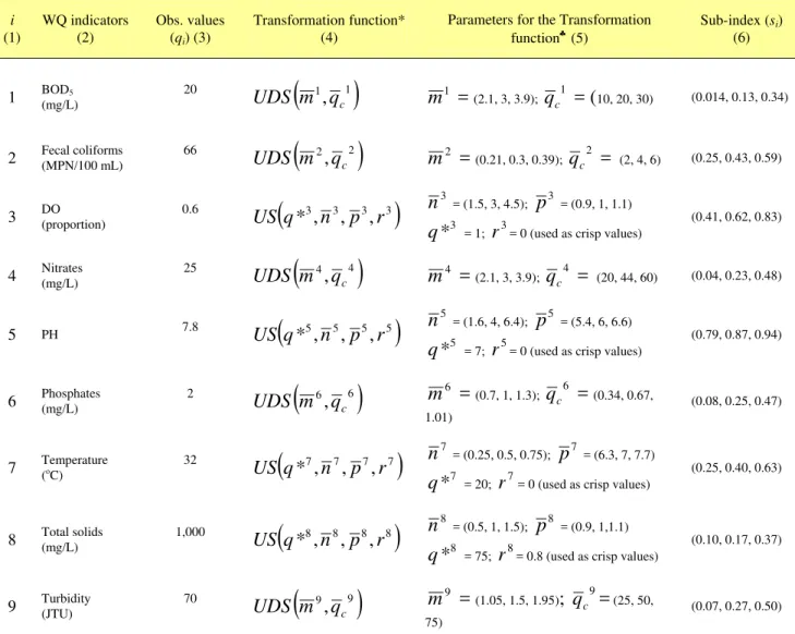
Water quality index (WQI) is a common tool used to classify lakes, streams and other fresh water sources, which translate a large amount of non-commensurate data into a single value (Ott 1978). For this purpose various regulated physico-chemical, microbiological and aesthetic water quality indicators are used. To demonstrate the use of proposed method raw water quality data are modified from Swamee and Tyagi (2000) and presented in Table 3.

The raw water quality data in Swamee and Tyagi (2000) consists of nine water quality indicators (sub-indices) including BOD5, fecal coliform, dissolved oxygen proportion with respect to saturation (DO), nitrates, pH, phosphates, temperature, total solids, and turbidity. As the units of various water quality indicators are non-commensurate, transformation functions are used to translate the actual values into an interval of [0, 1], where “0” corresponds to the worst value and “1” corresponds to the best value. For example for DO, ‘higher’ proportion means a ‘higher’ value of sub-index (i.e. a benefit criterion). Conversely, for fecal coliform, ‘higher’ concentration refers to a ‘lower’ value of sub-index and vice versa (i.e. a cost criterion). Therefore, an appropriate transformation function is required for each water quality indicator to map actual values over a normalized interval [0, 1]. Swamee and Tyagi (2000) proposed various transformation functions, including uniform deceasing sub-indices (UDS) and unimodal sub-indices (US). These transformation functions are defined deterministically, i.e., an actual value of a specific water quality indicator corresponds to a single transformed value over a normalized interval [0, 1]. The transformation functions are modified in this paper such as that an actual value of a specific water quality indicator corresponds to a

triangular fuzzy number (TFN). As it was argued in the introduction, this is more realistic because perception of the fuzzy ‘acceptability’ of quality even for a crisp value inputs of a water quality indicator.

The column 2 in Table 3 describes nine water quality indicators used in the analysis. Columns 4 and 5 provide the corresponding transformation functions and the associated parameters, respectively. To modify the transformation functions as fuzzy numbers, the associated parameters (Column 5) are defined as triangular fuzzy number using three vertices (a, b, c), which represent the minimum, most

likely and maximum values, respectively. To obtain fuzzy transformation function, fuzzy arithmetic

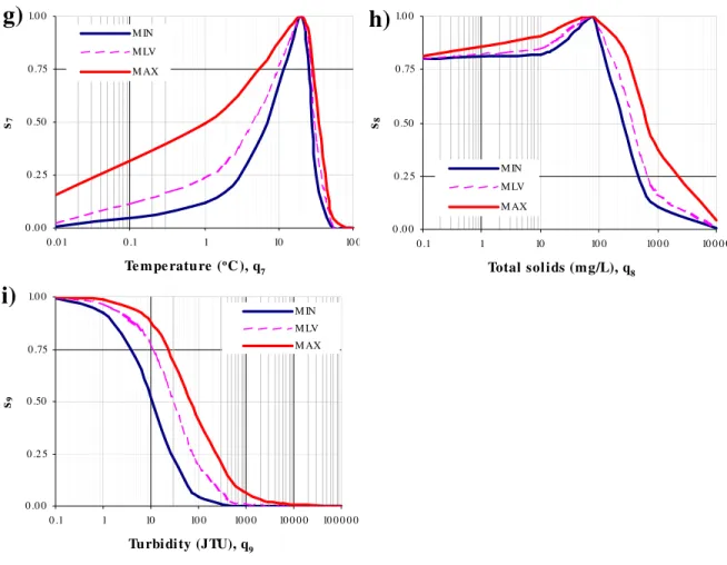
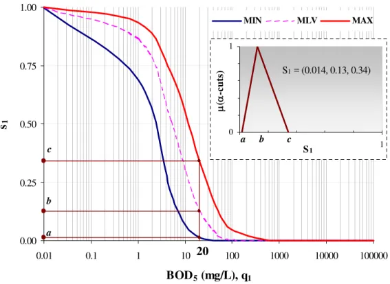
is employed as described earlier section. The fuzzy transformation functions for these nine water quality indicators are plotted in Figure 3. Therefore for crisp sub-index value, a transformed fuzzy

number is obtained. For example, for a BOD5 = 20 mg/L, after transformation, the corresponding S1 values becomes (0.014, 0.13, 0.34), which represent minimum, most likely, and maximum values respectively (Figure 4). For each of the nine water quality indicators, the input values qi given in

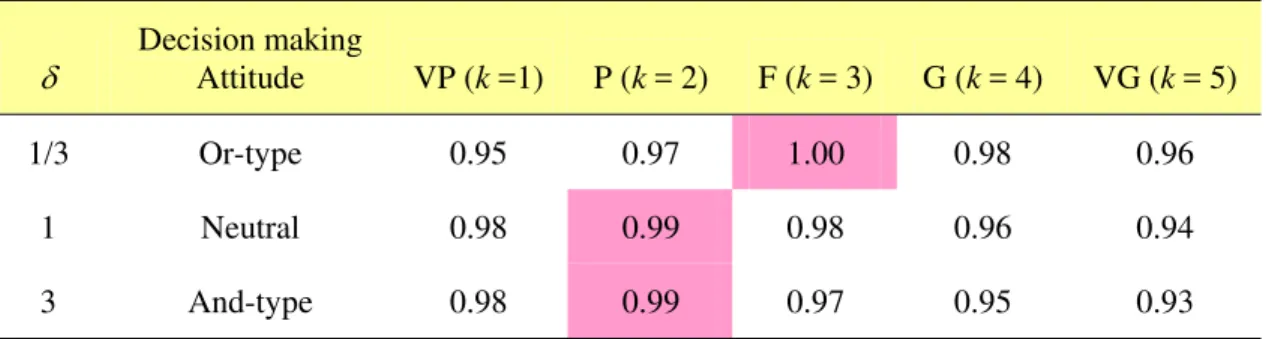
column 3 of Table 3 are transformed and also provided in column 6 of Table 3. These fuzzy numbers are now used for the proposed method FN-OWA to determine WQI (or an environmental index). The FN-OWA methodology is applied to three attitudinal scenarios; δ = 1/3 (or-type), δ = 1

(neutral) and δ = 3 (and-type). The corresponding orness values are computed as β = 0.76, 0.5, and 0.22, respectively. The results of water quality index are plotted in Figure 5, and the corresponding SMs are summarized in Table 4. It can be noticed that with an increase in δ value (or decrease in

orness β ), the EI values becomes smaller and vice versa (Figure 5). Therefore, the smaller orness values (β <0.5) accounts for an optimistic decision maker’s attitude and larger orness values (β >0.5) represents a pessimistic decision maker’s attitude. Table 4 shows that, with neutral and and-type decision attitude, the WQI is classified as poor, whereas, with or-type decision making attitude, the WQI is classified as fair.

These three scenarios may be a surrogate for the intended use of the water, e.g., recreational (fishing, swimming), irrigation, and drinking, respectively. Let’s assume a stream or a river that is used as a source of drinking water supply to a city, and its quality being monitored and evaluated for this purpose. The adverse consequences of even a marginal quality of source water for drinking water supply can be quite high, as a result, the decision maker will be conservative (or pessimistic) that necessitates selecting higher orness value (β >0.5). Conversely, if the primary use of source water is recreational, the smaller orness value (β <0.5) can be adopted.

DISCUSSION

Development of environmental indices is of paramount importance for engineers, managers and decision makers who deal with regulations and guidelines for environmental protection and

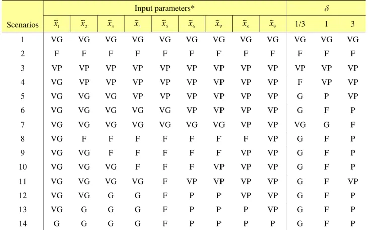
sustainable growth. The FN-OWA operator has ability to efficiently aggregate not only quantitative (crisp, interval, fuzzy) but also linguistic data. To illustrate the utility of the proposed approach, we

generated 14 scenarios in which each of the nine input parameters ( ) is defined

linguistically (Table 5) using ZFNs in Table 2. The nine input parameters are aggregated using three

9 2 1 ~ ,..., ~ , ~_{x x x}

estimated values of EI are converted into appropriate linguistic constant using similarity measure (SM) (Equation 6). The calculated SM for each linguistic constant is provided in Appendix.

For reliable decision-making, exaggeration and eclipsing are two major concerns encountered in the aggregation process. The 14 scenarios reported in Table 5 are used to illustrate the performance of the FN-OWA operator in terms of eclipsing and exaggeration. For the first three scenarios, same qualitative values (i.e., either VG, F, or VP) are selected for all nine input parameters. As was expected, the EI evaluated for nine input parameters for three different attitudes maintains the property of idempotency of FN-OWA operator. This implies that if all environmental quality indicators have same ‘state’, the overall environmental quality will retain that ‘state’.

Scenario 4 presents a case when only one indicator is VG and remaining 8 indicators are VP. The effect of this one environmental quality indicator is only captured, when δ = 1/3, which has shifted the EI to F. Now, as more environmental quality indicator were assigned better states (e.g., VG) in a step-by-step manner (from Scenarios 5 to 7), the EI for δ = 3, shifts from state VP to F, which means that the results are eclipsed by ‘poorer’ states of some of the environmental quality indicators. On the other hand, for δ = 1/3, the Scenario 5 represents a case in which only three indicators were in the VG state, but the EI hopped to state G, which is hinting an exaggeration. The compromising or risk neutral results were obtained when δ = 1 is selected.

In Scenarios 8 to 14, various states for environmental quality indicators are chosen. In Scenario 8, the δ = 1/3 provides an optimistic (i.e., EI is G) whereas δ = 3 provides a pessimistic picture (EI is P or VP). Similar observations can be made for the remaining Scenarios. However, it is interesting to note that the overall evaluation of EI does not change when δ = 1 due to symmetry of states for environmental quality indicators around middle input parameter ~x . ₅

By selecting δ = 1/3 (or-type), the decision-maker relies on those environmental quality indicators, which are performing ‘best’. Similarly, for δ = 3 (and-type), the decision-maker relies on the environmental quality indicators, which are performing ‘worst’. For δ = 1 (neutral), the decision-maker surmise a compromising attitude. Therefore, the FN-OWA operator provides flexibility in handling exaggeration and eclipsing in the computation of EI. The selection of appropriate value of risk attitude (δ) can also be linked to various levels of susceptibilities of environmental systems or to their intended beneficial use or to their importance.

The interpretation of environmental indices using OWA operators is context dependent. Throughout this paper, the input parameters were first transformed as “quality indicators” or “benefit criterion” before OWA aggregation. Therefore, larger orness values (β >0.5) lead to “optimistic”, whereas smaller orness values (β <0.5) lead to “pessimistic” decision-making attitudes. However, if all input parameters are transformed into “cost criterion” before OWA aggregation, the above logic reverses, which is the case of “environmental pollution” indices.

SUMMARY AND CONCLUSIONS

Environmental indices (EIs) are used as a communication tool to describe overall status of

environmental system. The computation of EI entails aggregation of different environmental quality indicators. In the final aggregation process, two potential pitfalls, exaggeration and eclipsing, are of paramount importance. The tolerance for these two pitfalls is often conflicting. However, using a flexible aggregation technique, the tolerance level for these two pitfalls can be incorporated into decision-making process.

The OWA operator is a generalized averaging operator that provides flexible aggregation ranging between the minimum and the maximum operators. The OWA operators allow incorporating decision maker’s attitude in the aggregation process. The availability of type of data and the interpretation of environmental indices are prone to vagueness. But, traditional OWA operators entail the use of crisp numbers (or fuzzy singletons), which is extended to fuzzy numbers also called FN-OWA. The utility of the proposed method to develop environmental indices are demonstrated using a vector of 9 input parameters.

Following observations and conclusions can be made:

• The FN-OWA operator provides a flexible aggregation ranging between the minimum and the

maximum operators for fuzzy (or qualitative) data.

• The FN-OWA operator has ability to aggregate not only the quantitative data, but can also handle linguistic as well as crisp data.

• The FN-OWA operator can help in explaining the fuzziness in meaning of ‘acceptability’ of quality for environmental indicators.

• The FN-OWA operator can also handle the missing information efficiently, i.e., a case of complete ignorance about the value of a given input parameter.

• The FN-OWA operator provides flexibility in handling exaggeration and eclipsing in the

aggregation process. For ‘benefit criteria’, by selecting δ < 1 (or-type), the decision-maker relies on those environmental quality indicators, which are performing ‘best’ and by selecting δ > 1 (and-type), the decision-maker relies on the environmental quality indicators, which are performing ‘worst’. For ‘cost criteria’ this argument is reversed.

• The aggregated value (estimated EI) obtained through FN-OWA operator retains the same linguistic state as if all input criteria have equal values, i.e., idempotency property of the FN-OWA operator.

REFERENCES

Ahn, B.S. (2006). The uncertain OWA aggregation with weighted functions having constant level of orness. International Journal of Intelligent System, 21: 469-483.

Carlsson, C. and Fullér, R. (2000). Benchmarking in linguistic importance weighted aggregation. Fuzzy Sets and Systems, 114: 35-41.

Chang, J.-R., Ho, T.-H. , Cheng, C.-H. and Chen, A.-P. (2006). Dynamic fuzzy OWA model for group multiple criteria decision making. Soft Computing - A Fusion of Foundations,

Methodologies and Applications, 10(7): 543 – 554.

Chang, N.B., Chen, H.W., and Ning, S.K. (2001). Identification of river water quality using the fuzzy synthetic evaluation approach. Journal of Environmental Management, 63: 293–305. Chen, S.-M. (1996). New methods for subjective mental workload assessment and fuzzy risk

analysis. Cybernetics and Systems: An International Journal, 27: 449-472.

Chen, S.-J. and Chen, S.-M. (2003a). A new method for handling multicriteria fuzzy decision-making problems using FN-IOWA operators. Cybernetic and Systems: An International Journal, 34: 109-137.

Chen, S.-J and Chen, S.-M. (2003b). Fuzzy risk analysis based on similarity measures of generalized fuzzy numbers. IEEE Transactions on Fuzzy Systems, 11(1): 45-56.

Chen, S.-J. and Chen, S.-M. (2005). Aggregating fuzzy opinions in the heterogonous group decision-making environment. Cybernetic and Systems: An International Journal, 36: 309-338.

Dubois, F., and Parade, H. (1988). Possibility theory: an approach to computerized processing of uncertainty. Plenum Press, New York.

Ferson, S. and Hajagos, J.G. (2004). Arithmetic with uncertain numbers: rigorous and (often) best possible answers. Reliability Engineering and Systems Safety, 85: 135-152.

Klir, G. J. and Yuan, B. (1995). Fuzzy Sets and Fuzzy Logic: Theory and Applications. Upper Saddle River, NJ: Prentice Hall International.

Lu, R.-S., and Lo, S.-L. (2002). Diagnosing reservoir water quality using self-organizing maps and fuzzy theory. Water Research, 36: 2265–2274.

Lu, R.-S., Lo, S.-L., Hu, J.-Y. (1999). Analysis of reservoir water quality using fuzzy synthetic evaluation. Stochastic Environmental Research on Risk Assessment, 13(5) : 327–36. Makropoulos, C.K. and Butler, D. (2006). Spatial ordered weighted averaging: Incorporating

spatially variable attitude towards risk in spatial multicriteria decision-making. Environmental Modelling & Software, 21(1): 69–84.

Mitchell, H.B. and Estrakh, D.D. (1998). OWA operator with fuzzy ranks. International Journal of Intelligent System, 13(1): 69-81.

Ott, W.R. (1978). Environmental Indices: Theory and Practice. Ann Arbor Science Publishers, Michigan, US.

Prodanovic, P. and Simonovic, S.P. (2002). Comparison of fuzzy set ranking methods for

implementation in water resources decision-making. Canadian Journal of Civil Engineering, 29: 692-701.

Sadiq, R., and Rodriguez, M.J. (2004). Fuzzy synthetic evaluation of disinfection by-products – a risk-based indexing system. Journal of Environmental Management, 73(1): 1-13.

Sadiq, R., Rodriguez, M.J., Imran, S.A., and Najjaran, H. (2007). Communicating human health risks associated with disinfection byproducts in drinking water supplies: a fuzzy-based approach. Stochastic Environmental Research and Risk Assessment, 21(4): 341-353.

Sadiq, R., and Tesfamariam, S. (2007) Ordered weighted averaging (OWA) operators for developing water quality indices using probabilistic density functions. Accepted in European Journal of Operational Research, 182(3): 1350-1368.

Silvert, W. (2000). Fuzzy indices of environmental conditions. Ecological Modeling, 130: 111-119. Smith, P.N. (2006). Flexible aggregation in multiple attribute decision making: application to the

Kuranda Range road upgrade. Cybernetics and Systems: An International Journal, 37: 1–22. Somlikova, R., and Wachowiak, M.P. (2001). Aggregation operators for selection problems. Fuzzy

Sets and Systems, 131: 23-34.

Swamee, P.K. and Tyagi, A. (2000). Describing water quality with aggregate index. ASCE Journal of Environmental Engineering, 126(5): 451-455.

Tao, Y., and Xinmiao, Y. (1998). Fuzzy comprehensive assessment, fuzzy clustering analysis and its application for urban traffic environment quality evaluation. Transportation Research, 3(1): 51– 57.

Xu, Z.S. and Da, Q.L. (2002). The uncertain OWA operator. International Journal of Intelligent Systems, 17: 569–575.

Yager, R.R. (1988). On ordered weighted averaging aggregation in multicriteria decision making. IEEE Transactions on Systems, Man and Cybernetics, 18: 183-190.

Yager R.R. (1996). Quantifier guided aggregation using OWA operators. International Journal of Intelligent Systems, 11: 49–73.

Yager, R.R. and Filev, D.P. (1994). Parameterized "andlike" and "orlike" OWA operators. International Journal of General Systems, 22: 297-316.

Table 1. Common arithmetic operations used in interval analysis

Operators ‡Formulae †Results

Summation A + B [a1 + b1, a2 + b2] = [5, 15] Subtraction A – B [a1 – b2, a2 – b1] = [1, 5] Multiplication A x B [a1 x b1, a2x b2] = [6, 50] Division A / B [a1/b2, a2/b1] = [0.6, 5] Scalar product Q · B [Q · b1, Q · b2] =[4, 10] a1 < a2; b1 < b2; ai andbi (i = 1 to 2) > 0; Q > 0 † A=[a1, a2] = [3, 10]; B=[b1, b2] = [2, 5]; Q = 2 ‡

Note: The values of A and B are positive, if negative numbers are used, the corresponding min and max values have to be selected.

Table 2. ZFNs defined to represent five linguistic constants (k) Linguistic constants (k) ak bk ck dk Very poor (VP) 0.0 0.0 0.05 0.25 Poor (P) 0.05 0.25 0.35 0.45 Fair (F) 0.35 0.45 0.55 0.65 Good (G) 0.55 0.65 0.70 0.95 Very good (VG) 0.70 0.95 1.00 1.00

Table 3 Transformation of raw water quality data into fuzzy sub-indices (modified after Swamee and Tyagi 2000)

i (1) WQ indicators (2) Obs. values (qi) (3) Transformation function* (4)

Parameters for the Transformation function♣ (5) Sub-index (si) (6) 1 BOD5 (mg/L) 20

(

1 1

)

,q_c m UDS m = 1 (2.1, 3, 3.9); q_c1 = (10, 20, 30) (0.014, 0.13, 0.34)

2 Fecal coliforms _{(MPN/100 mL)} 66 UDS

(

m2,q_c2

)

_{m =} 2

(0.21, 0.3, 0.39); q_c2 = (2, 4, 6) (0.25, 0.43, 0.59) 3 DO _(proportion) 0.6 US

(

q*3,n3,p3,r3

)

3 n = (1.5, 3, 4.5); p3 = (0.9, 1, 1.1) = 1; 3 *

q r3= 0 (used as crisp values)

(0.41, 0.62, 0.83) 4 Nitrates _(mg/L) 25 UDS

(

m4,q_c4

)

m = 4 (2.1, 3, 3.9); q_c4 = (20, 44, 60) (0.04, 0.23, 0.48) 5 PH 7.8 _US

(

_q*5_,n5_,p5_,r5

)

5 n = (1.6, 4, 6.4); p5 = (5.4, 6, 6.6) = 7; 5 *

q r5= 0 (used as crisp values)

(0.79, 0.87, 0.94) 6 Phosphates _(mg/L) 2 UDS

(

m6,q_c6

)

m = 6 (0.7, 1, 1.3); 6 c q = (0.34, 0.67, 1.01) (0.08, 0.25, 0.47) 7 Temperature ₍o_C) 32

(

7 7 7 7

)

, , , * n p r q US 7 n = (0.25, 0.5, 0.75); p7 = (6.3, 7, 7.7) = 20; 7 * q _r7

= 0 (used as crisp values)

(0.25, 0.40, 0.63) 8 Total solids _(mg/L) 1,000 US

(

q*8,n8,p8,r8

)

8 n = (0.5, 1, 1.5); p8 = (0.9, 1,1.1) = 75; 8 * q _r8

= 0.8 (used as crisp values)

(0.10, 0.17, 0.37)

9 Turbidity _(JTU) 70 UDS

(

m9,q_c9

)

m = 9 (1.05, 1.5, 1.95);

9

c

q = (25, 50, 75)

(0.07, 0.27, 0.50)

*Two types of transformation functions are used; UDS: uniform decreasing sub-indices; US: unimodal sub-indices

(

)

_i m c i i c i q q q m UDS − ⎟⎟ ⎠ ⎞ ⎜⎜ ⎝ ⎛ + = 1 , ;

(

)

(

)( )

(

)

i ni pi i i i i i n i i i i i i i i i i i q q r n p q q r p n r p r p n q US ₊ ⎟⎟ ⎠ ⎞ ⎜⎜ ⎝ ⎛ − + ⎟⎟ ⎠ ⎞ ⎜⎜ ⎝ ⎛ − + + = * 1 * 1 , , , *

Table 4. Assigning linguistic constants to WQI using similarity measures (SM)

δ Decision making Attitude VP (k =1) P (k = 2) F (k = 3) G (k = 4) VG (k = 5)

1/3 Or-type 0.95 0.97 1.00 0.98 0.96

1 Neutral 0.98 0.99 0.98 0.96 0.94

3 And-type 0.98 0.99 0.97 0.95 0.93

Table 5. Scenario analyses Input parameters* δ Scenarios 1 ~ x 2 ~ x 3 ~_x 4 ~ x 5 ~ x 6 ~_x 7 ~ x 8 ~ x 9 ~_{x 1/3 1 3} 1 VG VG VG VG VG VG VG VG VG VG VG VG 2 F F F F F F F F F F F F 3 VP VP VP VP VP VP VP VP VP VP VP VP 4 VG VP VP VP VP VP VP VP VP F VP VP 5 VG VG VG VP VP VP VP VP VP G P VP 6 VG VG VG VG VG VP VP VP VP G F P 7 VG VG VG VG VG VG VG VP VP VG G F 8 VG F F F F F F F VP G F P 9 VG VG F F F F F VP VP G F P 10 VG VG VG F F F VP VP VP G F P 11 VG VG VG VG F VP VP VP VP G F VP 12 VG VG G G F P P VP VP G F P 13 VG G G G F P P P VP G F P 14 G G G G F P P P P G F P

0.0 0.2 0.4 0.6 0.8 1.0 0.0 0.2 0.4 0.6 0.8 1.0

Environmental Index (EI)

μ ( α − cu ts)

0.0 0.2 0.4 0.6 0.8 1.0 0.0 0.2 0.4 0.6 0.8 1.0

Environmental index (EI)

μ (α -c u ts ) VP P F G VG aEI b_EI c_EI d_EI

0 .0 0 0 .2 5 0 .50 0 .75 1.0 0 0 .0 1 0 .1 1 10 10 0

Dissolve d oxyge n (proportion), q₃

s3 M IN M LV M AX 0 .0 0 0 .2 5 0 .50 0 .75 1.0 0 0 .1 1 10 10 0 pH, q5 s5 M IN M LV M AX 0 .0 0 0 .2 5 0 .50 0 .75 1.0 0 0 .0 0 1 0 .0 1 0 .1 1 10 10 0 10 0 0 Phosphate s (mg/L), q₆ s6 M IN M LV M AX 0 .0 0 0 .2 5 0 .50 0 .75 1.0 0 0 .0 1 0 .1 1 10 10 0 10 0 0 10 0 0 0 Ni trate s (mg/L), q₄ s4 M IN M LV M AX 0 .0 0 0 .2 5 0 .50 0 .75 1.0 0 0 .0 1 0 .1 1 10 10 0 10 0 0 10 0 0 0 BO D5 (mg/L), q1 s1 M IN M LV M AX 0 .0 0 0 .2 5 0 .50 0 .75 1.0 0 0 .0 1 1 10 0 10 0 0 0 10 0 0 0 0 0 Fe cal C ol iform (MPN/100ml), q2 s2 M IN M LV M AX

a)

_b)

c) d)

e) f)

0 .0 0 0 .2 5 0 .50 0 .75 1.0 0 0 .0 1 0 .1 1 10 10 0 Te mpe rature (o_{C ), q} 7 s7 M IN M LV M AX 0 .0 0 0 .2 5 0 .50 0 .75 1.0 0 0 .1 1 10 10 0 10 0 0 10 0 0 0 Total solids (mg/L), q8 s8 M IN M LV M AX 0 .0 0 0 .2 5 0 .50 0 .75 1.0 0 0 .1 1 10 10 0 10 0 0 10 0 0 0 10 0 0 0 0 Turbidity (JTU), q9 s9 M IN M LV M AX

g)

_h)

i)

Figure 3. Fuzzy transformation functions used for various water quality indicators (modified after Swamee and Tyagi 2000)

0.00 0.25 0.50 0.75 1.00 0.01 0.1 1 10 100 1000 10000 100000 BOD5 (mg/L), q1 s1 MIN MLV MAX b c a 20 0 1 0 1 S1 b c a S1 = (0.014, 0.13, 0.34) μ( α -cuts)

0 0.2 0.4 0.6 0.8 1 0.0 0.2 0.4 0.6 0.8 1.0

Water Quality Index (WQI)

μ (α − cu ts) δ = 3 δ = 1/3 δ = 1 VP P F G VG

APPENDIX A – Similarity measures estimated for 14 scenarios δ = 1/3 Scenarios VP(k =1) P (k = 2) F (k = 3) G (k = 4) VG (k = 5) 1 0.14 0.36 0.58 0.78 1.00 2 0.56 0.78 1.00 0.80 0.58 3 1.00 0.79 0.57 0.36 0.14 4 0.59 0.80 0.97 0.77 0.55 5 0.40 0.62 0.84 0.95 0.74 6 0.29 0.51 0.73 0.90 0.85 7 0.21 0.42 0.64 0.85 0.93 8 0.38 0.59 0.81 0.94 0.76 9 0.34 0.56 0.78 0.93 0.80 10 0.33 0.54 0.76 0.92 0.81 11 0.32 0.53 0.75 0.92 0.82 12 0.33 0.55 0.77 0.93 0.81 13 0.35 0.565 0.785 0.94 0.79 14 0.45 0.66 0.88 0.91 0.69 δ = 1 1 0.14 0.35 0.57 0.78 1.00 2 0.56 0.78 1.00 0.80 0.58 3 1.00 0.79 0.57 0.36 0.14 4 0.90 0.87 0.66 0.46 0.24 5 0.71 0.93 0.85 0.65 0.43 6 0.52 0.74 0.96 0.84 0.62 7 0.33 0.55 0.77 0.92 0.81 8 0.57 0.78 1.00 0.79 0.57 9 0.57 0.78 0.99 0.79 0.57 10 0.57 0.78 0.99 0.79 0.57 11 0.57 0.78 0.98 0.79 0.57 12 0.57 0.79 0.98 0.79 0.57 13 0.57 0.79 0.98 0.79 0.57 14 0.57 0.79 0.98 0.79 0.57 δ = 3 1 0.14 0.35 0.57 0.78 1.00 2 0.56 0.78 1.00 0.80 0.58 3 1.00 0.79 0.57 0.36 0.14 4 1.00 0.79 0.57 0.36 0.14 5 0.97 0.82 0.60 0.39 0.17 6 0.85 0.90 0.71 0.51 0.29 7 0.60 0.81 0.97 0.76 0.54 8 0.69 0.91 0.87 0.67 0.45 9 0.79 0.95 0.77 0.57 0.35 10 0.86 0.90 0.71 0.50 0.28 11 0.89 0.88 0.68 0.47 0.25 12 0.84 0.93 0.72 0.52 0.30 13 0.79 0.97 0.772 0.567 0.35 14 0.73 0.94 0.84 0.63 0.41