Atom Interferometry:
Dispersive Index of Refraction and
Rotation Induced Phase Shifts
for Matter-Waves
by
Troy Douglas Hammond
B.S., Milligan College (1989)
B.S., The Georgia Institute of Technology (1990)
Submitted to the Department of
Physics in partial fulfillment of
the requirements for the degree of
DOCTOR OF PHILOSOPHY
at the
MASSACHUSETTS INSTITUTE OF TECHNOLOGY
February 1997
© 1997 Massachusetts Institute of Technology
All rights reserved
Signature of Author
-Department of Physics
September 19, 1996
Certified by
David E. Pritchard
Professor of Physics
Accepted by
George F. Koster
.,,.::"-
:••n o,''Chairman, Department Committee
on Graduate Studies
FEB 121997
L1EIRARiESAtom Interferometry: Dispersive Index of Refraction and Rotation Induced Phase Shifts for Matter-Waves
by
Troy D. Hammond
Submitted to the Department of Physics on September 16, 1996, in partial fulfillment of the requirements for the degree of Doctor of Philosophy
Abstract
This thesis describes recent advances in the use of atom interferometers. The advances comprise two new techniques that will advance the ability of atom interferometers to make precision measurements and two experiments that demonstrate the extraordinary sensitivity of atom interferometers to rotations and to atom-atom interactions, respectively.
A novel scheme is described whereby multiple velocity components of an atomic beam contribute constructively to an atomic interference fringe pattern of large intensity. This multiplexing effect will allow the measurement of large dispersive phases in cases where the fringe would otherwise have damped out to zero contrast.
Amplitude diffraction gratings, the atom-optical elements which make up our atom interferometer, have been manufactured with unprecedented phase uniformity, or
coherence. A technique that utilizes registration marks to minimize drifts in the lithography of these gratings is described.
We have measured the sensitivity of our atom interferometer to rotations. Our results agree within experimental uncertainty of 1% with the theory predicted by the Sagnac effect. Further, we demonstrated a sensitivity four orders of magnitude better than that previously seen in an atom interferometer, approaching the sensitivity of the best commercially
available laser gyroscopes.
We have studied the velocity dependent index of refraction for sodium matter-waves passing through a dilute sample of Argon gas. Atom interferometers are the only devices able to detect the collision induced phase shift in atom-atom scattering. The phase shift was measured as a function of the velocity, or energy, of the incident sodium atomic beam allowing determination of the mid to long range interatomic potential.
Thesis Supervisor: Dr. David E. Pritchard Title: Professor of Physics
To
"I will not omit to relate another circumstance also, which is perhaps the most remarkable which has ever happened to any one. I do so in order to justify the divinity of God and of His secrets, who deigned to grant me that great favour; for ever since the time of my strange vision until now an aureole of glory (marvellous to relate) has rested on my head. This is visible to every sort of men to whom I have chosen to point it out; but those have been very few. This halo can be observed above my shadow in the morning from the rising of the sun for about two hours; and far better when the grass is drenched with dew. It is also visible at evening about sunset. I became aware of it in France at Paris; for the air in those parts is so much freer from mist, that one can see it there far better manifested than in Italy, mists being far more frequent among us. However, I am always able to see it and to show it to others, but not so well as in the country I have
mentioned."
Benvenuto Cellini (b.1500; d. 1571) [CEL27, p. 232]
Table of Contents
1. INTRODUCTION...8
A. Historical Background ... ... ... 8
B. The M .I.T. Interferometer ... ... ... . 12
2. PRECISE PHASE MEASUREMENT THROUGH MULTIPLEX VELO CITY SELECTION ... 25
A. Limits to Dispersive Phase Measurements ... 25
B. The Multiplex Velocity Technique ... 29
C. Results from Numerical Modeling ... ... 32
1. The Velocity Distribution ... 32
2. The Contrast and Phase ... 37
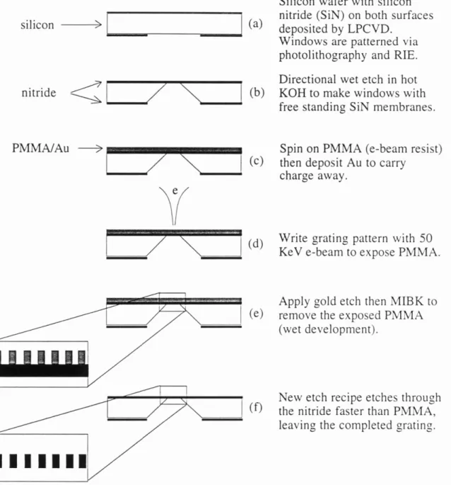
3. FABRICATION OF COHERENT AMPLITUDE DIFFRACTION G R A T IN G S ... 46
A. Grating Fabrication at the Cornell Nanofabrication Facility ... 46
B. Registration Marks for Improved Coherence ... ... 49
1. Field Stitching Errors ... ... 50
2. D rift Errors ... ... 54
3. Fabrication with Registration Marks ... . ... ... 54
4. Results ... ... 57
C. Large Area 100nm Period Gratings ... 59
1. Advantages of Optical Lithography over E-beam Lithography ... 59
4. MEASUREMENT OF ROTATIONS ... 69
A. The Sagnac Effect ... ... . ... 69
1. Sensitivity of an Interferometer to Non-Inertial Motion ... 69
2. History of the Sagnac Effect ... 70
3. Sensitivity Advantage of a Particle Interferometer ... 72
B. Rotation Sensing with an Atom Interferometer...74
1. A bstract ... 74
2. T he Paper ... 74
C. Experimental Details ... 83
1. Sensors ... 84
2. Forces and Constraints ... 87
D. Comparison of Sensors ... 91
5. VELOCITY DEPENDENT INDEX OF REFRACTION ... 93
A . Theory ... ... ... 93
1. Index of Refraction ... 93
2. The Atom-Atom Scattering Amplitude ... 94
3. Statistical Measurement ... ... 97
4.f(k,0) as a Sum Over Partial Waves ... 99
5. Analytical Results forf(k,0)...100
6. Numerical Calculation off(k,O) ... 102
7. Velocity Averagedf(k,O) ... ... 108
B. Experiment...114
1. Technical Advances in the Interferometer ... ... 114
2. Results: The Velocity Dependence of the Index of Refraction ... 118
APPENDICES
Appendix A: Multiplex Velocity Selection for Precision Matter-Wave
Interferom etry ... 124
Appendix B: Coherence of Large Gratings and Electon-Beam Fabrication Techniques for Atom-Wave Interferometry...129
Appendix C: Coherence and Structural Designs of Free-Standing Gratings for Atom-W ave Optics ... ... 136
Appendix D: The Phase of A Three Grating Interferometer ... 141
Appendix E: Phase Modulation Detection of the Inertial Phase ... 143
REFERENCES ... 144
1.
Introduction
A. Historical Background
In 1924, de Broglie proposed [DEB24] that every particle should exhibit wavelike behavior with a characteristic wavelength AdB = h/p, where h is Planck's constant and p
is the particle's momentum. Because of the small size of Planck's constant, wavelike effects are not generally observed for macroscopic particles. Indeed, for a thermal atom,
XdB is on the order of 10 picometers, at least an order of magnitude smaller than the size of the atom itself. However, it did not take long for this wave relation to be confirmed for electrons. In 1927, diffraction of electrons by crystals in both reflection [DAG27] and transmission [THR27] modes were observed. In 1930, diffraction of atoms was demonstrated by Estermann and Stem [ESS30] who reflected atoms off the closely spaced planes of a cleaved crystal surface.
The first complete matter-wave interferometer was demonstrated in the 1950's using electrons [MAR52, MSS54, MOD54]. In this interferometer, an electron beam was passed through thin crystals which acted as phase diffraction gratings. The electron interferometer was first demonstrated in a Mach-Zehnder configuration using transmission diffraction. This geometry is particularly forgiving for most alignment parameters. The 1960's and 1970's saw the development of neutron interferometers, first by using a biprism configuration [MAS62] and then by passing neutrons through crystals which act as diffraction gratings [RTB74]. Modem neutron interferometers, similar to Rauch's [RTB74], utilize a large single crystal of silicon with portions removed leaving behind three gratings. The angle of the crystal planes of these three gratings, with minor adjustments applied via differential heating, are then adequately aligned since they originate from a single crystal.
possible for atoms. In principle, atoms may be diffracted by reflection off crystal surfaces, however the alignment criteria on the three crystals are extraordinarily difficult to meet, although one group is currently trying [FRA93]. The idea and desire to build an interferometer for atoms is not new. It was patented in 1973 [ALF73] and since that time, it has been extensively discussed and reviewed [CDK85, BOR89, APB92, JDP94]. The potential benefits of developing an interferometer for atoms were numerous: large beam intensities, an interfering particle with rich internal structure, a wide range of properties for different atoms (e.g. mass, magnetic moment, polarizability, absorption frequencies), and a variety of strong interactions with the environment (e.g. with static electric and magnetic fields, radiation, and other atoms). Given that atom source and detector technology has been around for some time, the delay in the demonstration of an atom interferometer is attributed solely to the lack of suitable atom-optical elements with which to build the interferometer.
Suitable beam splitters were developed in the 1980's in Professor David E. Pritchard's research group at M.I.T. Diffraction of an atomic beam was demonstrated from a standing wave of resonant light (a phase grating) [MGA83] and from a slotted membrane (an amplitude grating) [KSS88]. Pritchard's group decided to pursue the construction of an atom interferometer with the amplitude diffraction gratings, and a successful demonstration of interference was achieved in early 1991. The diffraction gratings used were manufactured at the National Nanofabrication Facility at Cornell University using a process described in detail in Chapter 3. They essentially consist of an array of alternating bars and slots with an extremely small period of a few hundred nanometers.
The success of this interferometer and of several other types of atom interferometers has been one of the major developments in atomic physics of the 1990's. The demonstration of atomic interference in a Young's double slit experiment was presented by the Mlynek research group of Konstanz, Germany in late 1990. Soon thereafter the three grating interferometer developed at M.I.T. worked for the first time and the subsequent
papers appeared together in Physical Review Letters in May, 1991 [CAM91, KET91]. A variety of interferometers have now been proposed and realized. While the previously discussed two interferometers operated solely by affecting the atom's center of mass coordinates, two experiments that entangled the atom's internal and external degrees of freedom were demonstrated in 1991, at Stanford [KAC91] and at Braunschweig [RKW91]. These experiments were essentially optical analogs of Ramsey's separated oscillatory fields experiments and are now called interferometers. Atom interference has been demonstrated since then in a variety of contexts, including a longitudinal Stern-Gerlach experiment [RMB91], a two slit experiment using atoms dropped from a MOT (magneto-optical trap) [SST92], a 4-zone optical Ramsey experiment [SSM92], a near field three grating interferometer related to the Talbot effect [CLL94], and finally interferometers utilizing Kapitza-Dirac diffraction [ROB95] and Bragg scattering [GML95] from standing light waves. Proposed future interferometers include using helium diffraction from cleaved crystal surfaces [FRA93], diffraction from a time-dependent evanescent wave [HSK94, SGA96], and Bragg diffraction with cold atoms from a magneto-optic trap [RAI96].
The M.I.T. interferometer is unique in its physical separation of the beam paths. This allows the construction of an interaction region with a thin foil between the two paths so that interactions may be applied to only one path. Our research group at M.I.T., in recent years, has completed a number of experiments utilizing this new tool of separated beam atom interferometry. The first was the measurement of the static (d.c.) electric polarizability of the sodium atom with a precision of 0.35% [ESC95]. This is a factor of 20 improvement over previous measurements [HAZ74] and is more precise than the current state of the art in theoretical atomic structure calculations (1%) [LIU89].
The second experiment was the first ever measurement of the collision induced phase shift in atom-atom scattering [SCE95]. The phase shift experienced by a sodium beam passing through various gas samples, including the noble gases, was measured as a function of the density of the gas sample. In contrast to spectroscopic experiments, this
experiment is uniquely sensitive to the mid to long-range potential.
We have performed another experiment in which we applied differential magnetic fields to the two beam paths causing a rapid dephasing or loss of contrast as the different hyperfine ground states, which have different projections of magnetic moment, acquired different amounts of phase shift [SEC94]. At particular values of the magnetic field, all the states received the same phase modulo 21r and a sharp contrast revival occurred. We call this "contrast interferometry."
We have demonstrated near field interference with our diffraction gratings using the Talbot effect [CEH95a] and have also demonstrated that our interferometer works with molecules, specifically the sodium dimer Na2 [CEH95b]. This further extends the size and
complexity of particles that have been shown to interfere in accordance with de Broglie's wave hypothesis.
Finally, we have completed a detailed study of the loss of coherence that occurs when an atom in an interferometer scatters a single photon [CHL95]. This is a realization of the Feynman gedanken experiment, which was originally discussed in the context of an electron traversing a double slit [FLS63]. The experiment was then extended to show that the contrast is not lost but is just entangled with the reservoir of final photon states. We demonstrated that this contrast can be "found" or regained by performing a correlation experiment.
The outline of this thesis is as follows. The next section is a review of the details of our experimental apparatus, focusing on recent changes that have been made. In the second chapter I present a generalization of the "contrast interferometry" technique that will provide dramatic improvements in the precision measurement of certain dispersive phase shifts. In Chapter three, I discuss the techniques we have developed to fabricate amplitude diffraction gratings for our interferometer. These gratings are the key atom-optical elements on which our interferometer is based, and advances we recently made in their quality and size made possible our experiment measuring rotations which is then described
in Chapter four. In Chapter five, I describe an extension of the atom-atom collision induced phase shift experiment. We have measured the velocity dependence of this phase shift, allowing accurate determination of the mid to long-range potential between the sodium atom and a noble gas atom. Finally, I conclude in Chapter 6 with a discussion of some future atom interferometry experimental ideas.
B. The M.I.T. Interferometer
The M.I.T. atom interferometer is described in detail in [KET91] and in previous theses from this group [KEI91, EKS93, CHA95]. Here I will give an overview of the experimental apparatus, noting recent modifications.
It is often mentioned that our interferometer is of a Mach-Zehnder geometry. However the standard light Mach-Zehnder interferometer people are likely to come across, in an introductory physics laboratory for example, looks only vaguely similar. This interferometer consists of a partially silvered mirror which transmits and reflects portions of the incident beam, and the two resulting beams are then redirected toward each other with mirrors. Finally, another partially silvered mirror is placed at the beam's point of intersection completing the interferometer. (Figure 1.1A) The relative path length difference determines which port the light exits.
The first use of diffraction gratings as the beam amplitude splitting device, instead of partially silvered mirrors, is attributed to Carl Barus [BARl1]. (Figure 1.1B) The first use of diffraction gratings replacing the mirrors, or beam redirectors, was done by Marton et. al. [MSS54] in his demonstration of an electron interferometer. (Figure 1.1C) This latter addition has the very significant result that the fringes are now achromatic, or "white" [SIM56]. Only in the sense that our interferometer includes a beam amplitude splitter, a beam recombiner, and then another beam amplitude splitter, is it analogous to the original Mach-Zehnder geometry.
stainless steel reservoir containing sodium, typically pressured with 2 atm. of argon gas and heated to 7000C. A supersonic expansion out of the small 70 gm diameter nozzle produces an intense cold beam of sodium atoms entrained in the predominantly argon carrier beam [HAB77]. It has been proposed that the scattering from background gas has
(A;
(C)
Source 1
woos-~IFML
Figure 1.1 (A) The traditional Mach-Zehnder geometry interferometer. The source is typically a laser and passes first through a beamsplitter, then bounces off mirrors, and finally recombines at a beamsplitter. (B) A similar interferometer where diffraction gratings are now used as the beam splitters. (C) The geometry first used by Marton to build an electron interferometer, where a grating also serves as the beam recombiner in the middle. This is the geometry used in the M.I.T. atom interferometer. Multiple closed interferometer paths are formed by the many diffracted orders. The two most typically used are shown.
LOM - ... I - -000 0110 000
Source
Chamber
Differential
Chamber
Sodium Reseri
T-700
0C
2 atm. Argoi
Differential
Chamber
To Main
Chamber
Pump
Pump
Pump
Main Chamber
Detector
From
Differential
Slil
Chamber
Pump
rump
Main Chamber: Top View Showing Atom Beams
I
-
t Sodium I Beam 0th +1stInteraction
Region
I
Ist
-1sti
I
_1SUTo
DetectorGratings
Figure 1.2 The top part of the schematic details the source end of our atomic beam machine. Typical pressures, in torr, are indicated in each chamber. The first and second differential pumping chambers are necessary to remove the large gas load that results from the supersonic beam. The resulting atomic beam passes into the main chamber (continued in the middle schematic). This is the heart of the interferometer, containing the optical elements and any necessary interaction region. The detector chamber to the right is cold trapped with liquid nitrogen to maintain low pressure and background count rate. The lower graphs details the diffracted orders (solid lines) used in our interferometer. Other orders (-1st and others not shown) generally do not contribute to the interference pattern. This graph is dramatically not to scale. The gratings are separated by 66cm and the beam paths are separated by only 561.tm at the middle grating.
----
---been affecting our beam intensity (source chamber pressure was typically 10 millitorr). We have recently replaced the source chamber Stokes diffusion pump (4 inch throat) with a Varian (NRC) VHS-6 belly-shaped diffusion pump (8 inch throat). This improved the pressure in the main chamber by 1-2 orders of magnitude, allowing a Bayert-Alpert type ionization gauge to remain lit (-5x10⁻⁴ torr) in
spite of the large argon gas load from the source (-0.5 torr-liter/sec).
We were surprised to observe that in just a few days of operation, a layer of crystalline diffusion pump oil several millimeters thick can form on the inner surface of the belly portion of this pump. (DC705 very low vapor pressure oil
11
Copper
Heater
Skimmer
I
is used.) Apparently, sodium causes the Figure 1.3 Cross section of the new skimmer
mount. The skimmer is made of Rhodium
degradation/polymerization of the pump oil into plated Nickel and is heated to -5000C in operation. The stainless steel support acts as
a form that is solid at room temperature. Thus an insulator to minimize heat flow to the
chamber wall. Typical ambient pressures in the jet of oil vapor can crystallize on the cold the source (nozzle) chamber and the first
differential pumping chamber (on the left) are
belly-section of the pump wall instead of directly 5x10⁻⁴ and 5x10⁻⁶ torr respectively. condensing to the liquid form. It is found to
readily melt and return to the oil reservoir with the simple application of a heat gun. Though this crystallization may increase backstreaming, it does not appear to significantly affect the pump performance until or unless all of the oil is either trapped in this form or has backstreamed into the source chamber. At this point, just as a pot of boiling water can virtually burn up if all the water has boiled away, experience has shown that a diffusion
pump will melt-down when no oil remains.
The flange connecting the source chamber to the first differential pumping chamber has been replaced with one that allows an unrestricted expansion of the supersonic beam into the next chamber. (Figure 1.3) The skimmer (Beam Dynamics, Minneapolis, MN) which separates these two chambers is carefully mounted to allow uninhibited flow of the gas away from the beam line on both sides. A coaxial heater (ARI Industries, Addison, IL), similar to the heaters used on the source oven, maintains the skimmer at 300-4000C to prevent accumulation of sodium and possible clogging. In spite of the thin stainless tube connecting the heated skimmer to the chamber wall, the heat conduction to the wall is significantly larger than in the previous design which limited the contact to a ceramic macor spacer (macor is a machinable ceramic and an effective insulator) and three stainless steel screws. The increased power requirements resulted in burning out the skimmer heater twice in as many months. A more powerful heater was recently installed to alleviate this problem and a macor washer beneath the base of the skimmer is proposed to further reduce the power requirements.
The first differential pumping chamber (Varian HS-10 diffusion pump) and second differential pumping chamber (CVC-4 diffusion pump) eliminate most of the remaining gas load from the source, reducing the pressure to below 10-6 torr in the second differential chamber. Both chambers have optical access that was used for optical pumping and other manipulation of the beam in past experiments. Additionally, the first collimating slit is mounted on a translation stage in the first differential region.
Two types of collimating slits are used in our beam machine. Stainless steel "air slits", each 3 mm high, are available in 5, 10, and 25 gpm sizes (Melles Griot, Irvine, CA). Additionally, during our last trip to the National Nanofabrication Facility at Cornell University, we used standard photolithographic techniques to produce arrays of slits in a pure silicon wafer. Typical slit widths on a single chip from the silicon wafer are 15, 25,
Figure 1.4 Transmission Electron Micrograph (TEM) of a diffraction grating that we made at the National Nanofabrication Facility of Cornell University in the fall of 1994. The support structure has a periodof 5Jlm and an open fraction of 70%. The grating bars themselves have a period of 160nm (most of our experiments utilized 200nm period gratings) and a typical open fraction of 30-60%. The membrane shown is about l00nm thick (into the page). The construction details are included in Chapter 3.
in the main chamber, 78cm downstream of the first) are mounted on translation stages and can be moved during operation of the experiment to select the desired slit size. The fITst slit is now heated to prevent clogging from the substantial sodium beam and from oil that backstreams from the unbaffled 10" diffusion pump directly below.
The interaction ("main") chamber of our apparatus contains the three amplitude diffraction gratings that are the atom-optical elements for our interferometer (Figure 1.4).
A pressure of -5xlO-7 torr is maintainedby a 4 inch (Varian VHS-4) diffusion pump. A
cold-water baffle is used to minimize oil backstreaming which would slowly clog the diffraction gratings. It is an unfortunate situation, given the time and effort involved in
producing, mounting, and aligning these gratings, that vacuum accidents can and have caused damaging oil backstreaming. This completely clogs the gratings rendering them useless. Recently, heaters were added to each of the three grating mounts to reduce the gradual clogging of the gratings by sodium and oil. However, even with the gratings at
200°C, a blast of oil from the diffusion pump is fatal for the gratings.
The gratings are mounted on translation stages so they can be moved in or out of
105
4 2 O 4o
S810
o
C.)
210
38
6 4 -; --- ·- ··-- -- ---- ;---- ·-- y- .- ...--. .... ... ... .. ... -.... .... ...- ... .... .. . .. ...
--
.
.
.
---
..
'--
...
.
.
.
..
.
.
.
..
.
.
.
-600 -400 -200
0
200
400
600
Detector position (gtm)
Figure 1.5 Diffraction of atoms from the first grating in our apparatus as seen by scanning our 50glm wide detector which is in the far field. The plot is shown on a log scale to demonstrate the higher orders; most of the intensity resides in the central three orders. The solid line is a least squares fit to the data, which is
used to determine the velocity and the velocity width of the sodium beam. Typically only the central (Oth)
order and one of the first diffracted orders is used in the interferometer.
the beamline. With the second and third gratings removed from the beamline, a diffraction pattern from the first grating is observed by scanning the detector (Figure 1.5). The zeroth and one of the first diffracted orders (which will be refered to as +1 or -1) are normally the only ones that contribute to an interference pattern. The +1 and -1 diffracted orders from the second grating recombine at the plane of the third grating (bottom Figure 1.2), forming an interference pattern of sodium atoms with the same period as the diffraction gratings. The period is the same because the angle with which they approach is determined by
18
--
---
---
---
---
----
·-·-···-
~ ;. ... .... ... .... .1 . .... ... .... .... ... .... . - --. --.--.--.--. .. . . . .. .. .. .. ... .. ... . ... . L·' ··- · --- ----·--r ___ ·----· ·-·--- -- ·- · m -- ·-- ·---- _i ·--- ---··--·--- --- --- --- -- -- -- -- .. .... ... .. .... ... .... . .. .. ... .... ... ....... ... . .. .... ... .... . ... ... .... ... .. ----~ --- -__.~ - .... ... ... ... .... ... .... ... ... .~ ----~--- --- -- ... --- · . ...---- " . .... .. : --·--.. ....-- -- --- ---- ----... . .. ... ... . .. ... .. .. .. .. .... .. .. . ... . . . . .---
----. .... .. ... . . .. ... ... ... ... ..... . . .: ... .. . . .. . . ... ... -~ ~ ~ ~ ~ ~ ~ ~ ~ ~ ~ ~ la l t s l ar i n 1 1 1 1 1 es i l .... .... i l i s i
I
I
I
I
+1 -1 Beams From 2nd Grating 3rdGratingI
Figure 1.6 Schematic of the interference that occurs in the region of the third grating. The two plane waves (wavelength -O.16A) converge at a shallow angle (-10-4 radians) forming an interference pattern with a
period equal to the grating period (i.e. 160nm). The third grating acts as a mask: if it is positioned to block the maxima, a minimum intensity is transmitted; as it is scanned transversely to a position where it blocks the minima, a maximum is transmitted. Thus the interference pattern of Figure 1.7 is recorded at the detector to the right which is -300 grating bars (50jlm) wide.
diffraction from the first and second gratings which have the same period. (Figure 1.6) Though a very narrow detector could measure this interference pattern directly, a third grating is used to mask the pattern, providing a much greater signal and minimal loss in contrast.
Optical diffraction gratings, for a Helium-Neon laser interferometer, are mounted on the same translation stages as the atom gratings. This interferometer serves two purposes. First, the signal can be used to measure the relative positions of our matter
gratings thus determining the phase of the atom interferometer. Second, a servo mechanism is set up through a piezoelectric transducer (PZT) to drive the position of the middle grating. This allows us to lock the relative alignment of the gratings using the side of an optical fringe, dramatically reducing the effect of vibrations on the atom interferometer. I will discuss these vibrational effects more thoroughly after completing this survey of the experimental apparatus.
The atom beam enters the detector chamber through a small hole which maintains differential pumping to keep the detector chamber below l1x10 -7. The detector is a 50gtm
diameter hot Rhenium filament with a work function greater than the ionization potential of the sodium atom. The sodium atom hits the wire and, after a time delay of typically one millisecond or less, becomes ionized as the electron tunnels into the metal. Static electric fields then focus the ion into a high gain channel electron multiplier or C.E.M. (model 4831G, Galileo Inc., Sturbridge, MA) which produces a current pulse for the detected single ions. These pulses are then fed, along with positional information from the laser interferometer signal, into the data acquisition/recording system where they are counted.
This detector is highly selective to atoms with small ionization potentials, like alkalis. Thus most background gases will not be ionized or detected. It was found that cold trapping the detector chamber (pumped with a Varian V-80A turbomolecular pump) with liquid nitrogen reduces the pressure from -2x10 -7 torr to -5x10 - 8 torr and reduces the
background count rate by 2-3 orders of magnitude. It is possible that this dramatic improvement in background for a relatively minor decrease in vacuum pressure comes from trapping the residual background of sodium atoms that enter the detector chamber in the undetected portions of the beam. Sodium would contribute background counts, yet is trapped readily at liquid nitrogen temperatures. Any background oil molecules from o-rings or from backstreaming from the main chamber that might contribute background counts is also readily trapped. Finally, to prepare for operation, the detector wire is "bathed" in oxygen (-1x10⁻⁴torr) for two minutes at a high temperature before it is slowly
4000
03000
o
2000
1000
0
-400nm
-200
0
200
400
Position (nm)
Figure 1.7 Oscillation in detected counts as a function of the relative position of the three gratings. This interferogram has a contrast of nearly 50%, and the phase was determined to 24mrad in 10 seconds.
stepped down to the operating temperature over two or more hours. This procedure reduces the background and improves the time response of the detection.
The atom count data are collected, binned, and then plotted versus position as recorded by the laser interferometer. (The acquisition software is LabView, by National Instruments, Austin, TX; the (excellent) analysis software is Igor Pro, Wavemetrics, Lake Oswego, OR and is available on the Macintosh platform only.) A typical resulting interference pattern is shown in Figure 1.7. The theoretical maximum contrast for our interferometer is never 100% because of the amplitude difference of the two beam paths. Depending on the specific configuration and beam parameters, a predicted contrast of 65%
is typical, and we have observed fringes with up to 50% contrast fringes. Considering the dramatic improvement in matter grating fidelity that we have made (Chapter 3), we assign most of this loss of contrast to residual transverse vibrations. With a mean count rate of
3000 cts/sec, the phase of this fringe can be measured to -25 milliradians in about 10 seconds.
Finally I will discuss a number of mechanical changes made to the apparatus in order to reduce vibrational noise. These changes were motivated by the need to apply forces that cause well understood non-inertial motion of the apparatus (Chapter 4) and by the need to operate the interferometer with smaller period diffraction gratings (Chapter 5).
We believe this list of noise sources is beneficial to anyone trying to reduce vibrations in an experimental vacuum apparatus.
The single most significant reduction in vibration came from hanging the entire beam machine and the frame on which it rests from a steel cable attached to the ceiling. This isolated the machine from building noise in general, including that which was transferred through the floor from our own roughing pumps. Simply hanging the pumps and leaving the interferometer on the floor proved inferior. The apparatus, which weighs approximately 600 kilograms, can easily be lowered to or raised off the floor with turnbuckles at each of the four corners.
The stability was further improved by removing the roughing pump lines from the wall and bolting them securely to the floor. It was found that the roughing lines transmitted a large amount of vibration to the apparatus from the wall of our building, which is essentially a thin membrane compared to the solid concrete floor. It had been my personal observation a year earlier that increases in the noise as recorded on the laser interferometer seemed to be correlated with wind gusts on a particularly stormy night.
Another major source of noise was the main diffusion pump which hangs from an elbow, cantilevered from the side of the main beam tube. Since all vibrations that entered there seemed to be dramatically amplified by this tuning fork, a brace was added from the base of the pump to the opposite side of the frame of the apparatus. The large and noisy 17 cfm Sargent-Welch roughing pump for this chamber was replaced by a small Varian SD-90, borrowed from the detector chamber, which is more than ample for the minor gas
load from this chamber. A smaller SD-40 roughing pump replaced the SD-90 at the detector chamber. All of these changes significantly reduced the amplitude of certain peaks in the noise spectrum.
Fourth, a large number of electrical cables needed to run our experiment were rerouted and many that were ancient history (on the time scale of a graduate student) were removed. It was found that a large bundle of cables that extended from the top of a tall rack of electronics over to the beam machine made a fairly rigid coupling between the two. The electronics rack is fairly unwieldy, so this eliminated substantial vibrations from being transferred readily to the machine.
Finally, we discovered that diffusion pumps in operation (with no moving parts!) were a substantial noise source themselves. We added an air reservoir upstream in the water lines, hoping to remove any pressure waves in the water due to the water pumps in the building itself, however no configuration or reservoir volume made any noticeable difference. It was found, however, that simply tapering down the water flow so that it is lukewarm in the return was a significant help, implicating flow turbulence as a noise source. Approximately half of the total noise attributed to the diffusion pumps was found to "turn on" as the pumps warmed up. We attribute this either to the vibrations of a pot of boiling oil, which is essentially what a diffusion pump is, or to thermal gradient induced "creaking." There is a substantial amount of audible "creaking" and "popping" at the base of a hot diffusion pump, even when it has nominally reached thermal equilibrium.
Though several of the noise sources above were found by hunting down particular spectral features, our standard measure of noise has always been the root mean square (rms) change in the relative position of the gratings, as measured by the laser interferometer in one millisecond. This is the approximate transit time for an atom through our interferometer, so we typically acquire atom counts and grating position data on this natural time scale. In the past, this displacement was typically 35-45 nm; with the above changes made, it is now 15-20 nm. The former value was adequate for an interferometer based on
200 nm period gratings. The latter was necessary for the experiments described in this thesis, will be necessary for use of even smaller 100 nm gratings, and also probably is the limit for what can be achieved with the present vacuum apparatus.
2.
Precise Phase Measurement Through Multiplex Velocity
Selection
In this chapter I will discuss a new technique we have developed that promises dramatic improvement in the precision accessible to interferometric measurement of dispersive phases. This method overcomes loss of contrast that occurs in the normal interferometric measurement of a large dispersive phase. A discussion of the details of our new Multiplex Velocity scheme [HPC95] is followed by results of numerical modeling that I have completed. The paper we have published on this subject is included in Appendix A.
A. Limits to Dispersive Phase Measurements
The phase shift, 0, that results from applying a potential to the atom in one arm of the interferometer can be written, in the JWKB approximation, as
S= (k-ko)dx.
(2.1)
Here, k and ko are the perturbed and unperturbed wavevectors, respectively. Note that the phase shift comes from the spatial part of the wavefunction exclusively, since we are considering a time independent, conservative potential. Next, if we restrict this discussion to potentials U(x) that are much smaller than the kinetic energy of the atom, which is approximately 0.1 eV, we can use an Eikonal approximation, expanding the wavevector to first order in U/E:
S=
2m(E - U(x)) dx - I
mE dx
(2.2)
=f
U
(x)dx
'= iU(x)dx
Av
where v is the velocity of the atom. Thus any interaction that is not itself a function of the velocity of the atom, such as interactions with an electric or magnetic field, will produce llv
dispersion in the phase shift.
Consider, in particular, the application of a constant electric field over some length
L' on one path of the atom interferometer. The energy shift for the atom in the electric
field is given by the quadratic Stark shift U(x)= - al 2 where a is the static ground state polarizability of the atom. Substituting this into Eqn. (2.2) gives a phase shift
=v 1 " 2
(2.3)
that clearly depends inversely on the velocity.
To see the ramifications of this dependence, I now calculate the expected interference pattern observed in an interferometer. The intensity of the interference pattern for a single atom (or a monochromatic beam) is written
I = Io (l+ Co cos(kgx- p(v))). (2.4)
Here ?(v) is the phase shift given by Eqn. 2.3, kg is the diffraction grating wavevector (which determines the wavevector of the interference pattern), I 0 is the mean intensity, Co is the contrast, and x is the transverse position in the plane of the third grating. Since there is no coherence between different atoms traversing the interferometer, the observed interference pattern is an incoherent sum of the interference patterns contributed by each atom. Thus, if P(v) is the normalized velocity distribution of the more realistic non-monochromatic atomic beam, the interference pattern is given by
I= 10(1 + Cof P(v)cos(kgx - (v))dv)
= I0 ( + Co f P(v)[cos(kgx)cos(o(v))+ sin(kgx) sin(o(v))])
= I0(1 + Co[cos(kgx)f P(v)cos(p(v))dv + sin(kgx)f P(v)sin((v))dv]) (2.5)
= 10 lo(1+ 2 + B2 C cos(kgx + tan -(B/A)))
= Io (l+Cobs cos(kgx+ ob)
A= P(v)cos(4(v))dv and B= P(v)sin(Q(v))dv. (2.6) The observed contrast and phase shift are, respectively, Cobs and Pobs.
The supersonic beam used in our experiments is accurately described by a Gaussian velocity distribution. That is,
-(v-vo) 2
1 2o2 , (2.7)
where vo is the mean velocity andao is the root mean square (rms) width. To see the effect of this velocity distribution, we need to utilize P(v) in the calculation of A and B. However, this cannot be done analytically as the argument of the sine and cosine is 1/v. That is, if the phase of the mean velocity vo is defined to be the constant
S=
1U(x)dx,
(2.8)
tvo
then we have A =
f
P(v)cos(oovo /v)dv. Expanding the argument of the cosine, volv, tofirst order in `0 yields c=s(ovo
l/v)
coso
V-Vo)).Using the standard
trigonometric identity to expand this cosine, and inserting Eqn. 2.7 into A (Eqn. 2.6), yieldsS -(V-VO) 2 -(**0)2
A= cos e 2o cos o) d( - vo)+ sin o e
2
sin(dv o) - voBy symmetry the second integral is zero. The first integral is found in standard tables and
the result is A=c eo2/2v02 -O 2 2/2v02
the result is A =cos oe- av/2vo. A similar calculation shows that B = sin oe- 4v/ 2v
Finally, to first order in v-v , we see that the observed contrast of the interference pattern
VS
is
Cobs = CO A2 + B2 =
Ce
2v . (2.9)That is, the visibility of the fringe decays as a Gaussian function of the applied phase q0 and with a phase width of vol vradians. Similar treatment of the observed phase yields
I d~ I.U 0.8 o 0.6 o U 0.4 0.2 0.0 0.0 -0.1 ÷ -0.2 -G- -0.3 -0.4 0 10 20 30 40 50 4(vo) in radians
Figure 2.1 The top figure shows the damping, or washing out, of the fringe contrast as a function of increasing applied phase (Eqn. 2.9). For the example shown, o/vo is 4%. This is a typical velocity width
for the sodium beam in our apparatus. The lower graph shows a numerical calculation of the difference between the observed phase shift 4
obs and the phase applied to the mean velocity atoms (vo). According to the first order approximation in the text, this should be zero (Eqn. 2.10). For the region shown, this phase difference is much less than 1% of the total phase.
4?obs = tan-1(B/A) = 0. (2.10)
That is, at this level of approximation there is no difference between the observed phase
and the phase shift o0 of atoms with the mean velocity vo. Keeping higher orders would
show that there is a small difference, but it is easier to calculate this deviation of Pobs from
0o numerically (Figure 2.1).
It is interesting to examine the significance of the rms width, vo/a v radians, of the
interference fringes. A shift in one path of the interferometer by vo/" v radians corresponds to a path length change of lc, where v0/lv = kolc. Thus,
Ic= 1 vo k0 1 (2.10)
ko a
kO ak ak
Here lc, called the coherence length of the atomic beam, sets the scale in terms of path
length change for the loss of visibility of the fringes. It is inversely proportional to ak, the width of the wavevector distribution of the atomic beam. For a beam with cr/v o = 4% rms
velocity width, that is vo /lav = 25, the coherence length is Ic = 3AdB =0.6
A.
In contrast, a typical optical laser has frequency 500 Thz and linewidth 5 Mhz, a ratio of 108, with a resulting coherence length on the order of 10 meters.Thus, interactions which alter the path length of the atoms by just a few de Broglie wavelengths are sufficient to wash out the resulting interference pattern. In the experiment we performed to measure the electric polarizability of sodium [ESC95], this limit was
reached with the application of about 1 kilovolt/cm to one path of the interferometer.
Since the phase error is limited by statistics, one would like to apply as large a phase shift as possible to improve the accuracy in measuring this effect. This can only be done by dramatically narrowing the (already narrow) velocity distribution of the beam with a velocity selector. For example, a series of appropriately aligned, spinning slotted disks will dramatically reduce the velocity width of the beam, but at great cost to the intensity of the beam. A solution to this problem envisioned by Prof. David E. Pritchard and thoroughly worked out by myself in the summer of 1994 will now be described.
B. The Multiplex Velocity Technique
Consider two "choppers," separated by a distance L, placed in the path of the atomic beam (Figure 2.2). These "choppers" might be either spinning, slotted disks or pulses of focused resonant laser light that deflect atoms out of the beam path. In either case, we assume that they chop in phase, at the same frequency. Qualitatively, what does
VL'
Atom Beam
" Chopping" Laser
-
-Figure 2.2 Diagram of an atom interferometer with a resonant laser beam acting as a chopper by deflecting atoms out of the beams. The choppers are separated by a length L and the interaction region, where a phase shift is applied, has length L'.
the velocity distribution look like? A fraction f, the open fraction, of the atoms will pass through the first chopper in pulses. Of these atoms, only those with specific discrete velocities will "survive" the second chopper. Thus, the velocity distribution must be a series of peaks.
Specifically, suppose the chopping frequency is 1/At. A particularly fast atom might traverse the distance L in one unit of time At, so it has velocity vl=L/At. A slower atom might require 40 units of time At, so it has velocity v40=L/(40At). In general, all
atoms that pass through the first chopper with velocities
L
vn = nAt (2.12)
will also pass through the second chopper. The time spent between the two choppers for these atoms is t,=nAt=Lv,.n
Now, consider a typical applied phase, the Stark phase, where the atoms experience an energy shift
a1 2 -hos (2.13)
while in the electric field. Using Eqn. 2.3, the applied phase is
L' L'
n = t.0s = -ms = nAt-mS (2.14)
On nO)S Vn At L (2.14)
vn L
where t, is the time spent in the interaction region of length L' by an atom of velocity vn (using Eqn. 2.12). Of course, the llvndispersion of the phase exists precisely because the
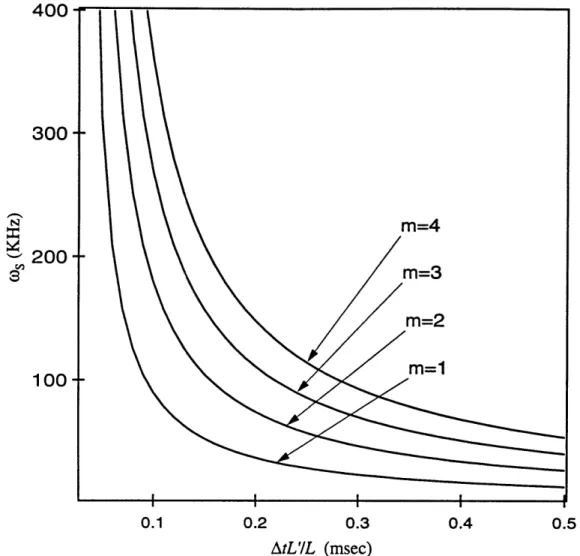
400 300 "-200 100 0.1 0.2 0.3 0.4 0.5 AtL'/L (msec)
Figure 2.3 A plot of the inverse relationship between the strength of the applied phase and the chopping period At that must be met for a rephasing using typical atomic beam parameters. Any point on any of these lines will generate a rephasing. A typical transit time through an interaction region 10cm in length is 0.1 msec.
time an atom spends in the interaction region accumulating a phase shift varies as llvn.
The key to the velocity multiplexing scheme, therefore, is that every atom in the beam spent a discrete number n of time units At traveling between the choppers and thus spends n units of time AtL'/ L in the interaction region. If cos is adjusted so that 27 radians of phase are applied in a time AtL'I L, then all atoms receive a phase that is a
multiple of 2rc. More generally, if os is adjusted such that LAtws = 2mn radians, with m
an integer, all the atoms receive a phase that is a multipe of 2xtm,
open
cnAt
time
Figure 2.4 The intensity transmitted through the chopper as a function of time.
This condition is shown graphically in Figure 2.3. When this condition is met, a rephasing will occur in the atomic interference contrast. Another way to explain this is that all atoms that would have acquired a phase nt plus a multiple of 2nr have been eliminated from the beam by the choppers. These atoms would have washed out the interference pattern had they remained in the beam with those that have a phase 0 plus a multiple of 27r, which pass through the choppers. It is this idea that a spectrum of different velocity components contributes constructively to the final signal that spawned the name "Velocity Multiplexing."
C. Results from Numerical Modeling
In this section I will take a more detailed look at the actual velocity distribution P(v) that results from the chopper. Then I will present the contrast and phase curves,
comparable to Figure 2.1, that result from this new distribution. Finally, I will discuss the limit to which the phase can be measured using this technique.
1. The Velocity Distribution
The fraction of atoms that passes through the first chopper is
f
Atopen (2.16)At
the open fraction of the chopper. (Figure 2.4) As we have noted, any of these atoms that has velocity exactly equal to vn (Eqn. 2.12) will pass through the second laser beam unobstructed. So the transmission T of atoms with these special velocities through both
chopping regions is justf, the open fraction of the laser beam.
To find the transmission T for some velocity v # vn, consider a pulse of atoms,
Atopen in duration, with this velocity that passes through the first chopper. The first atoms
from this pulse will reach the second region a time t=Llv later and the pulse will continue to arrive at region two until the time t+ Atopen. Let f' describe the extent to which the arrival
of this pulse of atoms is temporally offset from an opening at region two. That is, f' is the fraction of the pulse that gets blocked at the second chopper. The case v=vn
corresponds to f'=0. To the extent that tldAt is not integral, the pulse will be offset from an opening and a reduced fraction f-
f',
or none at all, of the atoms pass through. The resultsfor f' and Tare
f'=INT- and (2.17)
T=
f-lf' forlf'l
<f
(2.18)
By INT, I mean rounding the result to the nearest integer in the standard manner. So, of the fraction f of all atoms that pass through the first chopper, a fraction f' of these is blocked at the second region. This result assumes that If 5I 0.50 and that the chopper has negligible longitudinal length. With these approximations, this result agrees with a more general one in the excellent article on velocity selectors by Meijdenberg [MEI88].
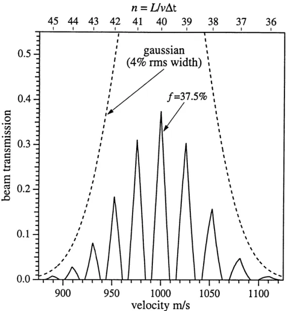
This transmission function is plotted in Figure 2.5. For the case shown, the laser choppers are assumed to be 10 cm apart, their period is 2.5 gsec, and the open fraction is 0.375. With these parameters, an atom would need a velocity of 40,000 m/s to reach the second chopper in one period. So, v1=40,000 m/sec. The top graph shows the transmission from zero velocity up to and including vl. The lower graph is an expansion of the top graph, showing the region of interest for our typical atomic beams at
v40= 1000 m/sec. Here the peaks are spread fairly uniformly and the 1/v dependence in
0.4
0.3
0.2
0.1
0.0
0.4
0.3
0.2
0.1
0.0
54 3
n = L/vAt
2
0
10000
20000
30000
40000
velocity (m/s)
n =
1/vAt45 44 43 42 41
40
39
38
37
36
900
950
1000
1050
1100
velocity (m/s)
Figure 2.5 The transmission function for the velocity chopper assuming 10cm separation, a 2.5 p.sec period, and a 0.375 open fraction. The top graphs shows the transmission at all velocities up to v,=l and the lower graph is an expansion around v--40.
The resulting velocity distribution for an atomic beam passing through this chopper just requires multiplying the beam's velocity distribution times this transmission function.
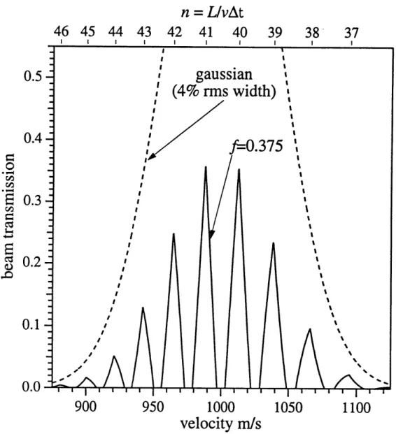
I have plotted this result for a realistic case in Figure 2.6. Our atomic beam has a Gaussian
profile, typically with a 4% rms width and the velocity centered at one kilometer per
few hundred Khz is required to produce multiple peaks under this Gaussian profile. This explains the period At=-2.5gtsec used in most of my calculations and would be easy to achieve experimentally by passing a laser beam chopper through an acousto-optic modulator (AOM). In this configuration, n=40 chopping periods occur during the transit time of the atoms with central velocity V40, which I also write as vo. The velocity distribution is plotted for a 37.5% open fraction. Since roughly a fractionf of all the atoms pass through the second laser beam, the integrated area under this velocity distribution is close tof 2, or 14%.
By referring to Figure 2.6, one can more easily understand the function of a
"conventional" velocity selector. A conventional velocity selector has additional chopping regions, for example slotted disks, positioned so as to remove all the side peaks shown in this figure. Only the central, narrow velocity peak remains. While this would serve the function, as described earlier, of dramatically increasing the coherence length of the beam, this would induce significant loss of beam intensity.
I will now quantify the improvement of signal that comes with the velocity multiplexing technique over the single peak of the conventional velocity selector. Assuming that there are at least several peaks in the velocity distribution, the ratio between the area under all the peaks and the area under the central peak of velocity v, is
f
2 JP(v)dv1 1 Ir n ov (2.19)
vn+1/2 P o) -n-1/2) 1 2fvo 2 fn+1/2 f vo
f
2
JP(v)dv
n
Vn-1/2
For the case off-r0.375, which we will see later is an optimum choice, and with n=40 and a 4% velocity width, this signal improvement factor is 5.3. From this equation it is obvious that two things, a larger n and a wider velocity width, yield a larger improvement factor. First, a larger n corresponds to a more finely chopped velocity distribution. The transmitted intensity for the multiplexed beam profile is proportional to
f2,
regardless of then =
L/vAt
45
44 43 42 41
40
39
38
37
36
0.5
0.4
O
0.3
S0.2
0.1
0.0
900
950
1000
1050
1100
velocity m/s
Figure 2.6 The velocity distribution P(v) for chopping regions with 37.5% open fraction. The dotted line is the Gaussian velocity profile that is incident on the chopper. Note the 1/v spacing of the peaks themselves, labeled by their integer n on the top axis.
number of peaks, while the single peak from the conventional selector steadily gets thinner with increasing n. The goal of increasing n would be to achieve finer resolution (apply larger phases) which costs no loss in the intensity of the multiplexed beam. In the second case, had the original velocity distribution been wider than 4%, it would have been more costly to achieve the same narrow velocity width with the conventional selector. But again, the multiplexing scheme takes full advantage of the entire velocity distribution.
I have devised a slightly more complex scheme that further extends the intensity advantage of the velocity multiplexing scheme. Note that the first chopper in any velocity
selector removes a fraction 1-f of the entire beam regardless of velocity. An optimal velocity selector would not do this, but instead produce peaks with their full original intensity. This can be achieved if f=0.50 and if, instead of chopping atoms, they are
tagged as they pass through region one. For instance, suppose the atoms have two ground
states A and B. The pulsed chopping laser is replaced by "it-pulses" that transfer atoms from state A to B or vice versa. Assume that all atoms arrive at the first interaction region in state A. Then, where atoms would have been removed when the laser pulse is on, they are instead just transferred to state B. If atoms in state B arrive at region two with the laser on (thus, they have the desired velocity), they will be transferred back to state A. Otherwise they remain in state B. Atoms in state A that arrive at region two when the laser is on do not have the desired velocities and are transferred to state B. The result is that all the atoms that have the desired velocities leave this new selector in state A. That is, all the atoms under the peaks in Figure 2.6 (the peaks would now extend to the full height of the Gaussian envelope) would be in state A while all the rest of the atoms would be in state B. These can then simply be removed further downstream with, for example, a deflecting laser that is only resonant with state B or with a deflecting Stern-Gerlach magnet. This "smart" velocity selector yields a factor two improvement in the signal to noise over the velocity multiplexing scheme with choppers.
2. The Contrast and Phase
Having thoroughly investigated the new multi-peaked velocity distribution P(v) that results from two choppers, we can now use it to calculate A and B numerically from Equation 2.6, which gives us the contrast and phase curves that would be experimentally observed. I use the phase that would be applied to an atom of velocity vo, 0(vo), as the independent variable in all these calculations. The calculated contrast is shown in Figure 2.7. The contrast revivals damp out at higher 0(vo), as we would expect, because the peaks of the velocity distribution still have a finite width. Correspondingly, the higher
1.0
0.8
0.6
o
U
0.4
0.2
0.0
n =(p(vo)/2n
0
20
40
60
80
100 120 140 160
0
200
400
600
800
1000
(p(vo) in radians
Figure 2.7 The contrast of the interference fringes as a function of phase applied to atoms with the mean velocity. Contrast revivals for several integral values of m and for three open fractions f are shown. The smaller open fractions (narrower peaks in the velocity distribution) have stronger revivals.
order revivals are strongest for the smallest open fractions, which have the narrowest peaks.
By examining the height of the first contrast revivals, I am now in a position to find the optimal open fraction f as determined by the resulting signal to noise. Assuming that
the noise is accurately described by Poissonian statistics, the interferometer signal to noise ratio (SNR) is
n = L/vAt
46 45 44 43 42
41
40
0.5
0.4
0.3
0.2
0.1
0.0
39
38
37
900
950
1000
1050
1100
velocity m/s
Figure 2.8 The velocity distribution P(v) for chopping regions with 37.5% open fraction. The chopping frequency is slightly higher so that the mean velocity vo=1000 m/s does not coincide with a peak in the distribution. Note that the n=40 peak has shifted to a higher velocity.
SNR = C- N = C-J (2.20)
with C the fringe contrast and N the mean count rate. In this case, the count rate N is actually fiN and, from fitting a line to the contrast (CoblCo) versus the open fraction (three points can be obtained from the first revival of Figure 2.7), C is roughly given by
Co(1.2-1.6f) in the rangef-0-.25 to
f-0.50.
The resulting SNR yields a broad maximum centeredat an open fraction off-r0.375.
0.8-o
0
.60.4
-0.2
0.0,
-3.0
0-a-n=(p (v
o )
/2it
32
34
36
38
40
42
44
46
48
S I I I I I I-3?5-
ILine fit
here S . . . . , . . . 0 I...
* i..*...*
..*
0 0 * I * 0 0 * * 0 . 0 * . 0 0 0 .* * . * , * 0 . * : 0:0: : :0 * ·. * : * . * 0 I I I I I I200
220
240
260
280
300
O(v
o)
in radians
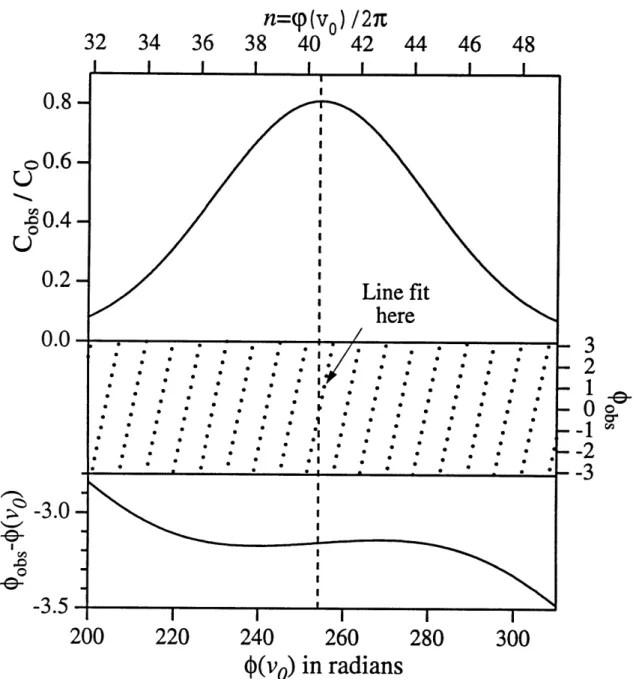
Figure 2.9 Detailed study of the first contrast revival from Figure 2.6. The top graph shows the contrast. The middle graph show the calculated observed phase. The lower graph is the difference between the observed phase and the phase applied to atoms with the mean velocity. A zero in the observed phase is found to align with the maximum of the contrast revival to better than 1 part in 10s.
frequency that creates the velocity distribution of Figure 2.6 results in a transit time of n=40 chopping periods for vo= 1000 m/sec atoms. Thus revivals occur at phases O(vo) equal to 40 times 2rtm radians. So, the peak m=1 in the figure lies at n=40.
In general, however, the mean velocity vo of the incident atom beam will not be a
peak in the velocity distribution after the choppers as it was in Figure 2.6. The position of
40