Preindustrial to present-day changes in tropospheric hydroxyl radical and methane lifetime from the Atmospheric Chemistry and Climate Model Intercomparison Project (ACCMIP)

(1)

HAL Id: hal-03048333

https://hal.archives-ouvertes.fr/hal-03048333

Submitted on 10 Dec 2020

HAL is a multi-disciplinary open access

archive for the deposit and dissemination of

sci-entific research documents, whether they are

pub-lished or not. The documents may come from

teaching and research institutions in France or

abroad, or from public or private research centers.

L’archive ouverte pluridisciplinaire HAL, est

destinée au dépôt et à la diffusion de documents

scientifiques de niveau recherche, publiés ou non,

émanant des établissements d’enseignement et de

recherche français ou étrangers, des laboratoires

publics ou privés.

Preindustrial to present-day changes in tropospheric

hydroxyl radical and methane lifetime from the

Atmospheric Chemistry and Climate Model

Intercomparison Project (ACCMIP)

V. Naik, A. Voulgarakis, A. Fiore, L. Horowitz, J.-F. Lamarque, M. Lin, M.

Prather, P. Young, D. Bergmann, P. Cameron-Smith, et al.

To cite this version:

V. Naik, A. Voulgarakis, A. Fiore, L. Horowitz, J.-F. Lamarque, et al.. Preindustrial to present-day

changes in tropospheric hydroxyl radical and methane lifetime from the Atmospheric Chemistry and

Climate Model Intercomparison Project (ACCMIP). Atmospheric Chemistry and Physics, European

Geosciences Union, 2013, 13 (10), pp.5277-5298. �10.5194/ACP-13-5277-2013�. �hal-03048333�

(2)

Atmos. Chem. Phys., 13, 5277–5298, 2013 www.atmos-chem-phys.net/13/5277/2013/ doi:10.5194/acp-13-5277-2013

EGU Journal Logos (RGB)

Advances in

Geosciences

Open Access

Natural Hazards

and Earth System

Sciences

Open Access

Annales

Geophysicae

Open Access

Nonlinear Processes

in Geophysics

Open Access

Atmospheric

Chemistry

and Physics

Open Access

Atmospheric

Chemistry

and Physics

Open Access Discussions

Atmospheric

Measurement

Techniques

Open Access

Atmospheric

Measurement

Techniques

Biogeosciences

Open Access Open Access

Biogeosciences

Discussions

Climate

of the Past

Climate

of the Past

Discussions

Earth System

Dynamics

Earth System

Dynamics

Discussions

Geoscientific

Instrumentation

Methods and

Data Systems

Open Access

_{Geoscientific}

Instrumentation

Methods and

Data Systems

Geoscientific

Model Development

Geoscientific

Model Development

Discussions

Hydrology and

Earth System

Sciences

Open Access

Hydrology and

Earth System

Sciences

Ocean Science

Discussions

Solid Earth

Discussions

The Cryosphere

Natural Hazards

and Earth System

Sciences

Open Access

Discussions

Preindustrial to present-day changes in tropospheric hydroxyl

radical and methane lifetime from the Atmospheric Chemistry and

Climate Model Intercomparison Project (ACCMIP)

V. Naik1, A. Voulgarakis2, A. M. Fiore3, L. W. Horowitz4, J.-F. Lamarque5, M. Lin4,6, M. J. Prather7, P. J. Young8,9,*, D. Bergmann10, P. J. Cameron-Smith10, I. Cionni11, W. J. Collins12,**, S. B. Dalsøren13, R. Doherty14, V. Eyring15, G. Faluvegi16, G. A. Folberth12, B. Josse17, Y. H. Lee16, I. A. MacKenzie14, T. Nagashima18, T. P. C. van Noije19, D. A. Plummer20, M. Righi15, S. T. Rumbold12, R. Skeie13, D. T. Shindell16, D. S. Stevenson14, S. Strode21, K. Sudo22, S. Szopa23, and G. Zeng24

1_{UCAR/NOAA Geophysical Fluid Dynamics Laboratory, Princeton, New Jersey, USA} 2_{Department of Physics, Imperial College, London, UK}

3_{Department of Earth and Environmental Sciences and Lamont-Doherty Earth Observatory of Columbia University,}

Palisades, New York, USA

4_{NOAA Geophysical Fluid Dynamics Laboratory, Princeton, New Jersey, USA} 5_{National Center for Atmospheric Research, Boulder, Colorado, USA}

6_{Atmospheric and Oceanic Sciences, Princeton University, New Jersey, USA}

7_{Department of Earth System Science, University of California, Irvine, California, USA}

8_{Cooperative Institute for Research in the Environmental Sciences, University of Colorado-Boulder, Boulder, Colorado, USA} 9_{Chemical Sciences Division, NOAA Earth System Research Laboratory, Boulder, Colorado, USA}

10_{Lawrence Livermore National Laboratory, Livermore, California, USA}

11_{Agenzia nazionale per le nuove tecnologie, l’energia e lo sviluppo economico sostenibile (ENEA), Bologna, Italy} 12_{Hadley Centre for Climate Prediction, Met Office, Exeter, UK}

13_{CICERO, Center for International Climate and Environmental Research-Oslo, Oslo, Norway} 14_{School of Geosciences, University of Edinburgh, Edinburgh, UK}

15_{Deutsches Zentrum für Luft- und Raumfahrt, Institut für Physik der Atmosphäre, Oberpfaffenhofen, Germany} 16_{NASA Goddard Institute for Space Studies, New York City, New York, USA}

17_{GAME/CNRM, Météo-France, CNRS – Centre National de Recherches Météorologiques, Toulouse, France} 18_{National Institute for Environmental Studies, Tsukuba-shi, Ibaraki, Japan}

19_{Royal Netherlands Meteorological Institute, De Bilt, the Netherlands}

20_{Canadian Centre for Climate Modeling and Analysis, Environment Canada, Victoria, British Columbia, Canada}

21_{NASA Goddard Space Flight Center, Greenbelt, Maryland, USA and Universities Space Research Association, Columbia,}

MD, USA

22_{Department of Earth and Environmental Science, Graduate School of Environmental Studies, Nagoya University,}

Nagoya, Japan

23_{Laboratoire des Sciences du Climat et de l’Environnement, LSCE/CEA/CNRS/UVSQ/IPSL, France} 24_{National Institute of Water and Atmospheric Research, Lauder, New Zealand}

*_{now at: Lancaster Environment Centre, Lancaster University, Lancaster, UK} **_{now at: Department of Meteorology, University of Reading, Reading, UK}

Correspondence to: V. Naik (vaishali.naik@noaa.gov)

(3)

5278 V. Naik et al.: Changes in tropospheric hydroxyl radical and methane lifetime

Abstract. We have analysed time-slice simulations from 17

global models, participating in the Atmospheric Chemistry and Climate Model Intercomparison Project (ACCMIP), to explore changes in present-day (2000) hydroxyl radical (OH) concentration and methane (CH4) lifetime relative to

prein-dustrial times (1850) and to 1980. A comparison of mod-eled and observation-derived methane and methyl chloro-form lifetimes suggests that the present-day global multi-model mean OH concentration is overestimated by 5 to 10 % but is within the range of uncertainties. The models con-sistently simulate higher OH concentrations in the North-ern Hemisphere (NH) compared with the SouthNorth-ern Hemi-sphere (SH) for the present-day (2000; inter-hemispheric ra-tios of 1.13 to 1.42), in contrast to observation-based ap-proaches which generally indicate higher OH in the SH al-though uncertainties are large. Evaluation of simulated car-bon monoxide (CO) concentrations, the primary sink for OH, against ground-based and satellite observations sug-gests low biases in the NH that may contribute to the high north–south OH asymmetry in the models. The models vary widely in their regional distribution of present-day OH con-centrations (up to 34 %). Despite large regional changes, the multi-model global mean (mass-weighted) OH concentra-tion changes little over the past 150 yr, due to concurrent in-creases in factors that enhance OH (humidity, tropospheric ozone, nitrogen oxide (NOx) emissions, and UV radiation

due to decreases in stratospheric ozone), compensated by in-creases in OH sinks (methane abundance, carbon monoxide and non-methane volatile organic carbon (NMVOC) emis-sions). The large inter-model diversity in the sign and mag-nitude of preindustrial to present-day OH changes (ranging from a decrease of 12.7 % to an increase of 14.6 %) indi-cate that uncertainty remains in our understanding of the long-term trends in OH and methane lifetime. We show that this diversity is largely explained by the different ratio of the change in global mean tropospheric CO and NOx

bur-dens (1CO/1NOx, approximately represents changes in OH

sinks versus changes in OH sources) in the models, pointing to a need for better constraints on natural precursor emis-sions and on the chemical mechanisms in the current gen-eration of chemistry-climate models. For the 1980 to 2000 period, we find that climate warming and a slight increase in mean OH (3.5 ± 2.2 %) leads to a 4.3 ± 1.9 % decrease in the methane lifetime. Analysing sensitivity simulations per-formed by 10 models, we find that preindustrial to present-day climate change decreased the methane lifetime by about four months, representing a negative feedback on the cli-mate system. Further, we analysed attribution experiments performed by a subset of models relative to 2000 conditions with only one precursor at a time set to 1860 levels. We find that global mean OH increased by 46.4 ± 12.2 % in response to preindustrial to present-day anthropogenic NOxemission

increases, and decreased by 17.3 ± 2.3 %, 7.6 ± 1.5 %, and 3.1 ± 3.0 % due to methane burden, and anthropogenic CO, and NMVOC emissions increases, respectively.

1 Introduction

The hydroxyl radical (OH) is the dominant oxidizing agent in the global troposphere as it reacts with most pollutants (Levy, 1971; Logan et al., 1981; Thompson, 1992), thereby controlling their atmospheric abundance and lifetime. Any changes in OH affect the tropospheric chemical lifetime of methane (CH4), the most abundant organic species in the

at-mosphere and a potent greenhouse gas, since reaction with OH is the primary mechanism by which it is removed from the atmosphere. Complex series of chemical reactions in-volving tropospheric ozone (O3), methane, carbon monoxide

(CO), non-methane volatile organic compounds (NMVOCs), and nitrogen oxides (NOx= NO + NO2), as well as the levels

of solar radiation and humidity, determine the tropospheric abundance of OH (Logan et al., 1981; Thompson, 1992). The more-than-doubling of global methane abundance since preindustrial times (Petit et al., 1999; Loulergue et al., 2008; Sapart et al., 2012), combined with the rise in emissions of NOx, CO and NMVOCs (Lamarque et al., 2010), is likely

to have had some influence on OH and consequently on the chemical methane lifetime in the past 150 yr. We analyse re-sults from global chemistry-climate models participating in the Atmospheric Chemistry and Climate Model Intercom-parison Project (ACCMIP; see www.giss.nasa.gov/projects/ accmip) to investigate the changes in tropospheric OH abun-dance and its drivers, and methane lifetime over the historical period between 1850 and 2000.

Primary production of tropospheric OH occurs when elec-tronically excited O(1D) atoms, produced by ozone photoly-sis at wavelengths less than 340 nm, react with water vapor:

O3+hν(λ <340 nm) → O(1D) + O2 (R1)

O(1D) + H2O → 2OH

. (R2)

Therefore, production of OH is highest in the tropical lower to middle troposphere, reflecting the combined impact of high levels of water vapour, and low stratospheric ozone col-umn, meaning higher incident ultraviolet (UV) radiation (Lo-gan et al., 1981; Spivakovsky et al., 2000; Lelieveld et al., 2002). OH has a tropospheric lifetime on the order of sec-onds, reacting rapidly with CO, methane and NMVOCs to produce HO2or an organic peroxy radical (RO2), key species

for the secondary production of OH:

OH + CO(+O2) →HO2+CO2 (R3)

OH + RH(+O2) →RO2+H2O

. (R4)

Secondary formation of OH can occur in the presence of NOx

since NO reacts with HO2or RO2 to recycle OH (Crutzen,

1973; Zimmerman et al., 1978):

HO2+NO → NO2+OH (R5)

RO2+NO(+O2) →R0CHO + NO2+OH

. (R6)

Additional OH is produced because NO2can photolyse

(4)

V. Naik et al.: Changes in tropospheric hydroxyl radical and methane lifetime 5279

OH (Hameed et al., 1979):

NO2+hν(λ<420 nm) → O(3P) + NO (R7)

O(3P) + O2+M → O3+M

. (R8)

This secondary production of OH via radical recycling by NOx (Reactions R5–R6) plays a more important role at

higher latitudes where incoming solar radiation and water vapour are less abundant, and NOxand ozone concentrations

are generally higher (Logan et al., 1981; Spivakovsky et al., 2000; Lelieveld et al., 2002). Conversely, in clean air the re-action chain can be terminated by the loss of HO2

(Reac-tion R3) and RO2radicals (Reaction R4) via

HO2+HO2→H2O2+O2 (R9)

RO2+HO2→ROOH + O2

. (R10)

Recent laboratory studies have indicated that reaction of se-lected RO2radicals with HO2can also produce OH at

sig-nificant yields (Dillon and Crowley, 2008 and references therein):

RO2+HO2→RO + OH + O2. (R11)

This has implications for NOxpoor, NMVOC rich

environ-ments where radical recycling via (R5) and (R6) is sup-pressed. Several chemical mechanisms, proposed for the cy-cling of HO2 to OH under low-NOx, high-NMVOC

con-ditions, are yet to satisfactorily reconcile discrepancies be-tween modeled and observed OH indicating large uncertain-ties in our understanding of the tropospheric photochemical oxidation (Stone et al., 2012 and references therein). Chem-ical mechanisms describing Reaction (R11) are not imple-mented in the models considered here. Temperature plays a key role by controlling reaction rates and tropospheric water vapour abundances. Overall, the global mean tropospheric OH represents a balance between its sources (water vapor, tropospheric ozone, NOxcontributing to secondary OH

pro-duction) and sinks (methane, CO, NMVOCs), that is modu-lated by overhead ozone column (UV radiation) and temper-ature.

The extent to which tropospheric OH level has changed due to anthropogenic activity is highly uncertain. Observa-tional evidence of preindustrial to present-day changes in OH is sparse and questionable. For example, Staffelbach et al. (1991) postulated that OH has decreased by 30 % in the present-day relative to preindustrial times using measure-ments of formaldehyde to methane (HCHO/CH4) ratio in

ice cores as potential proxy of the past OH concentration. However, Sofen et al. (2011) note that ice-core formalde-hyde is sensitive to post-depositional processing that im-pedes quantitative interpretation of past atmospheric condi-tions. Previous modeling of changes in tropospheric mean OH abundance from preindustrial to present-day range from increases of 6 to 15 % (Crutzen and Bruhl, 1993; Martinerie et al., 1995; Berntsen et al., 1997), to no change (Pinto and Khalil, 1991; Lelieveld et al., 2004), to decreases of 5 to

33 % (Thompson et al., 1992; Wang and Jacob, 1998; Mick-ley et al., 1999; Hauglustaine and Brasseur, 2001; Grenfell et al., 2001; Lelieveld et al., 2002; Shindell et al., 2003; Wong et al., 2004; Lamarque et al., 2005a; Shindell et al., 2006a; Skeie et al., 2010; Sofen et al., 2011; John et al., 2012). As evident from these wide-ranging results, there is no consen-sus on how tropospheric OH abundance has evolved in the past 150 years, with a consequent lack of agreement on the trends in methane lifetime during the historical period (Ta-ble 1 of John et al., 2012).

Much effort has been placed on understanding the long-term trends and interannual variability in atmospheric OH concentrations over the past two to three decades. Long-term site-specific measurements of OH concentrations provide in-sight on its trend/variability for specific chemical regimes (Rohrer and Berresheim, 2006). For an understanding of the changes in global mean OH, one must rely on measurements of trace gases whose emissions are well known and whose primary sink is OH. Accurate long-term measurements of the industrial chemical 1,1,1-trichloroethane (methyl chloro-form CH3CCl3) (Prinn et al., 1995, 2000, 2001; Montzka et

al., 2000) in the atmosphere and an assumption of accurate emissions inventories (Montzka and Fraser, 2003) enable es-timates of trends and interannual variability in tropospheric abundance of OH to be inferred from observed changes in CH3CCl3(Prinn et al., 1995, 2001, 2005; Krol et al., 1998;

Krol and Lelieveld, 2003; Bousquet et al., 2005; Montzka et al., 2000, 2011). Large changes in OH in the past three decades inferred from CH3CCl3 observations (Prinn et al.,

2001; Bousquet et al., 2005) have been debated in the litera-ture (Krol and Lelieveld, 2003; Lelieveld et al., 2004) as they have been difficult to reconcile based on results from cur-rent theoretical models that suggest small increases in global OH concentrations for the 1980–2000 period (Karlsd´ottir and Isaksen, 2000; Dentener et al., 2003; Dalsøren and Isaksen, 2006; Hess and Mahowald, 2009; John et al., 2012; Holmes et al., 2013). In a more recent analysis of CH3CCl3

mea-surements since 1998 (a period with diminished atmospheric CH3CCl3 gradients due to phasing out of its emissions

un-der the Montreal Protocol), Montzka et al. (2011) infer small interannual OH variability and attribute previously estimated large year-to-year OH variations before 1998 to uncertain-ties in CH3CCl3 emissions. Further, using observations of

methane and δ13C-CH4, Monteil et al. (2011) find that

mod-erate (< 5 %) increases in global OH are needed to explain the observed slowdown in the growth rate of atmospheric methane, thus incompatible with the previously estimated observation-based reduction in OH in 2000 relative to 1980. Previous multi-model studies have focused on inter-comparison of changes in atmospheric composition with ref-erence to OH and methane lifetime in the context of changes in ozone and CO (Stevenson et al., 2006; Shindell et al., 2006b). To our knowledge, our study provides the first multi-model estimates of historical OH changes, thereby demon-strating our current level of understanding of historical trends

(5)

in OH and methane lifetime based on the current generation of chemistry-climate models (CCMs). Here our goals are to (1) evaluate the present-day (2000) OH in the models, (2) ex-plore changes in OH and methane lifetimes since preindus-trial times, and (3) investigate the impact of individual fac-tors (climate and ozone precursor emissions) driving these changes. A parallel study compares future projections of OH and methane lifetime in the ACCMIP models (Voulgarakis et al., 2013). We provide a summary of models used, the exper-iments they performed, and our analysis approach in Sect. 2. Historical OH and methane lifetime are presented in Sect. 3. Changes in OH, methane lifetime, and their driving factors in the present-day (2000) relative to preindustrial (1850) and to 1980 are discussed in Sects. 4 and 5, respectively. The sen-sitivity of OH and methane lifetime to historical change in climate, and changes in methane burden and emissions are presented in Sects. 6 and 7, respectively, with conclusions drawn in Sect. 8.

2 Methodology

2.1 ACCMIP models

We analyse results from 17 different global models to inves-tigate how OH and methane lifetime in the present-day has changed relative to 1850 and to 1980. In other studies, AC-CMIP results have been analysed to compare changes in at-mospheric composition from 1850 to 2100 with a focus on physical climate variables (Lamarque et al., 2013), tropo-spheric ozone (Young et al., 2013) and its radiative forcing (Stevenson et al., 2013; Bowman et al., 2013), black carbon (Lee et al., 2013), and on aerosol radiative forcing (Shindell et al., 2013). Detailed descriptions of ACCMIP models are provided by Lamarque et al. (2013).

Nearly all the models are run as coupled chemistry-climate models (CCMs), driven by climatological monthly mean sea surface temperatures (SSTs) and sea ice coverage (SIC) ei-ther from observations or from the corresponding coupled ocean–atmosphere model integrations submitted to the Cou-pled Model Intercomparison Project Phase 5 (CMIP5). Three models, namely CICERO-OsloCTM2, MOCAGE, and TM5 are chemistry transport models (CTMs) driven by meteo-rological fields from an offline reanalysis or output from a general circulation model. Meteorological fields used to run CICERO-OsloCTM2 and TM5 did not vary across time-slice simulations. GISS-E2-R and GISS-E2-R-TOMAS are two different configurations of the same model – GISS-E2-R is a fully interactive coupled ocean–atmosphere-chemistry model with a simple mass-based representation of aerosols, while E2-R-TOMAS uses SSTs and SIC from GISS-E2-R with a more detailed aerosol microphysics scheme. Similarly, HadGEM2 and HadGEM2-ExtTC are the same, except HadGEM2 includes a simple tropospheric chemistry

scheme, while HadGEM2-ExtTC incorporates a more de-tailed chemistry scheme with many more hydrocarbons.

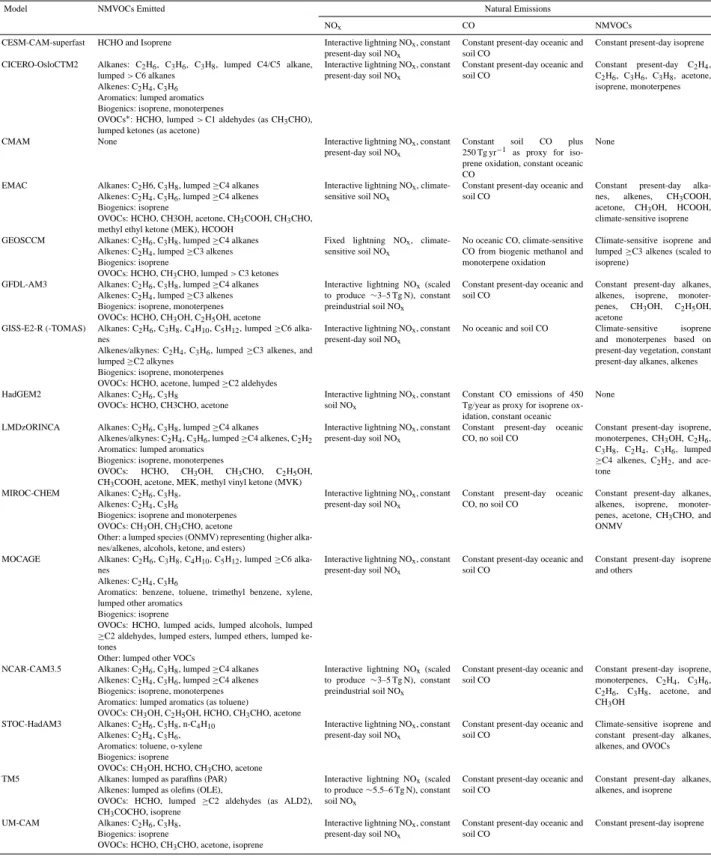
Key characteristics of the models relevant for simulating atmospheric OH and methane lifetime are presented in Ta-ble A1 of Voulgarakis et al. (2013). Briefly, anthropogenic and biomass burning emissions are taken from Lamarque et al. (2010) and vary over the historical period (Young et al., 2013). Natural emissions for NOx, CO, and NMVOCs were

specified from different sources and are one of the major sources of diversity in model results (Table A1; source-wise emissions for 2000 implemented in the models are summa-rized in Table S1 in the Supplement). Other sources of dif-ferences across the models are expected to result from diver-sity in the complexity of NMVOC chemistry (mechanisms include a range from 16 to 100 species), stratospheric ozone representations, and resulting impacts on ozone photolysis rates (see Table 3 of Lamarque et al. (2013) for further de-tails). Most models prescribe methane values at the surface (but allow it to undergo chemical processing elsewhere in the atmosphere) from the historical reconstruction of Mein-shausen et al. (2011) though a few models use alternative proaches. Two models (STOC-HadAM3 and UM-CAM) ap-ply a uniform global concentration and another (LMDzOR-INCA) applies emission fluxes. The temperature-dependent rate coefficient (kCH4+OH) for methane oxidation (R4)

ap-plied in most models is from Sander et al. (2011). Global and annual average kCH4+OH implemented in the models

are shown in Table S2 in the Supplement. The coefficient of variation (CV; standard deviation as a percentage of the multi-model mean) for kCH4+OH across models is less than

2 %, suggesting that the impact of differences in temperature across models on kCH4+OH is minimal and is, therefore,

un-likely to contribute to the diversity in methane lifetime shown later.

2.2 Simulations

We analysed three time-slice simulations over the histori-cal period – 1850, 1980 and 2000, performed by 16 mod-els (HadGEM2-ExtTC performed only attribution simula-tions described below). The models were typically run for 4 to 10 yr for each time-slice, though GEOSCCM performed 14 yr integrations, CICERO-OsloCTM2 and TM5 performed single year simulations (the reference year for TM5 present-day simulation being 2006), and GISS-E2-R and LMDzOR-INCA were run transiently for the entire historical period. For the analysis performed here, we averaged results over all the available years of each of the three historical time-slices. In the case of the GISS-E2-R and LMDzORINCA models, we averaged years centered on the time-slice (ex-cept average over 1850–1859 was used for 1850 and average over 1996–2000 was used for 2000 for LMDzORINCA). In-terannual variability in OH is not explicitly addressed here because ACCMIP simulations were designed to address only long-term changes.

(6)

Table 1. Global total methane burden, airmass-weighted tropospheric mean OH, and tropospheric methane lifetime (τ_CH4) for 1850, 1980 and 2000 time-slices, and tropospheric CH3CCl3lifetime (τMCF) for 2000 time-slice from 16 models. The troposphere is assumed to extend from surface to 200 hPa for each model’s grid. A cell with∗means that the model did not report that quantity. Multi-model mean (MMM) with standard deviation (STD), coefficient of variation (CV; standard deviation as percentage of the multi-model mean), and observation-derived estimates of τCH4 and τMCF(based on Prinn et al. (2005) and Prather et al.(2012)) are shown in the last three rows.

CH4Burden OH τCH4 τMCF

(Tg) (105molec cm−3) (years) (years)

Models 1850 1980 2000 1850 1980 2000 1850 1980 2000 2000 CESM-CAM-superfast (CE) 2191 4431 4902 12.1 12.3 12.8 9.3 8.8 8.4 4.9 CICERO-OsloCTM2 (CI) 2089 4286 4779 11.7 10.3 10.4 9.1 10.1 10.0 5.8 CMAM (CM) 2179 4260 4846 11.9 10.6 10.7 8.7 9.7 9.4 5.5 EMAC (EM) 2163 4235 4788 12.7 11.3 11.7 8.9 9.6 9.1 5.4 GEOSCCM (GE) 2178 4258 4818 13.0 11.3 11.3 8.6 9.7 9.6 5.6 GFDL-AM3 (GF) 2221 4234 4809 12.7 11.4 11.7 8.9 9.7 9.4 5.5 GISS-E2-R (GI) 2188 4226 4793 9.8 9.9 10.5 11.9 11.4 10.6 6.2 GISS-E2-R-TOMAS (GT) 2189 4499 4816 11.6 12.0 12.7 10.4 9.8 9.2 5.3 HadGEM2 (HA) 2155 4133 4680 8.1 7.8 8.1 11.6 12.1 11.6 6.7 LMDzORINCA (LM) 2293 4506 4980 11.0 10.2 10.3 10.1 10.7 10.5 6.1 MIROC-CHEM (MI) ∗ ∗ 4805 13.4 12.4 12.4 ∗ ∗ 8.7 5.1 MOCAGE (MO) 2126 4205 4678 11.6 12.5 13.3 8.2 7.5 7.1 4.1 NCAR-CAM3.5 (NC) 2209 4309 4903 10.7 11.3 12.0 10.7 9.9 9.2 5.4 STOC-HadAM3 (ST) 2127 4161 4708 11.8 11.6 12.1 9.7 9.6 9.1 5.3 TM5 (TM) 2173 ∗ 4820 10.9 ∗ 10.5 9.8 ∗ 9.9 5.8 UM-CAM (UM) 2209 4323 4879 7.0 7.1 7.4 15.0 14.7 14.0 8.4 MMM ± STD 2179 ± 47 4290 ± 115 4813 ± 81 11.3 ± 1.7 10.8 ± 1.6 11.1 ± 1.6 10.1 ± 1.7 10.2 ± 1.7 9.7 ± 1.5 5.7 ± 0.9 CV (%) 2.2 2.7 1.7 15.2 14.8 14.6 17.3 16.4 15.6 16.3 Observation-derived estimates 10.2+0.9_−0.7, 6.0+0.5_−0.4, (Prinn et al., 2005; 11.2 ± 1.3 6.3 ± 0.4 Prather et al., 2012)

Of the 17 models, 10 models performed an additional sim-ulation (Em2000Cl1850) with emissions fixed at 2000 levels, but with climate (SSTs and SIC) set to 1850 conditions (well-mixed greenhouse gases, including methane and ozone de-pleting substances (ODSs) were also set to 1850 levels for ra-diation calculations). The difference of Em2000Cl1850 from the 2000 simulation allows us to investigate the influence of historical climate change on global OH and the methane life-time. Furthermore, a few of these models performed a series of attribution experiments, specifically designed to ascribe ozone and OH changes to the increases in anthropogenic emissions of individual species (NOx, CO, NMVOCs) and to

the rise in methane concentrations (Stevenson et al., 2013).

2.3 Analysis approach

We calculate the tropospheric methane lifetime against loss by OH (τCH4) as the ratio of the global atmospheric methane

burden (BCH4) and the global annual mean tropospheric

methane–OH oxidation flux (LCH4) provided by each model

for each year and then averaged over the number of years for each time-slice. Hereafter, “methane lifetime” refers to the lifetime against loss by tropospheric OH (τCH4). The

to-tal methane lifetime additionally includes the small strato-spheric and soil sinks (Prather et al., 2001; Stevenson et al., 2006; Voulgarakis et al., 2013). For tropospheric global bud-gets, we define the troposphere to extend from the surface to a fixed pressure level of 200 hPa on each model’s native

verti-cal grid. We verti-calculated methane lifetime with the tropopause defined as air with ozone concentrations less than or equal to 150 ppbv in the 1850 time-slice simulation (Stevenson et al., 2006; Young et al., 2013) (Table S3 in Supplement) and found it to be within 1 % of the values obtained with the tropopause at 200 hPa (Table 1). Thus we conclude that the definition of the tropopause has minimal effect on the calcu-lated methane lifetime. With the exception of global budget terms, we weight global mean quantities reported here by the mass of air in each model grid cell.

We also calculate the tropospheric lifetime of CH3CCl3

against OH loss (τCH3CCl3) as a means of testing model

simulated global mean tropospheric OH concentrations for present-day. Since models did not simulate the chemistry and distribution of CH3CCl3, we calculate its tropospheric

life-time by scaling the methane lifelife-time with the ratio of the rate coefficient of the reactions of methane and CH3CCl3 with

OH (Prather and Spivakovsky, 1990) integrated from the sur-face to the tropopause as τCH3CCl3=τCH4

Rtrop

sfc kCH4+OH(T ) Rtrop

sfc kCH3CCl3+OH(T )

, where kCH3CCl3+OH(T ), the temperature-dependent rate

co-efficient for the oxidation of CH3CCl3by tropospheric OH is

1.64 × 10−12 exp(-1520/T ) molec−1cm3s−1(Sander et al., 2011). We apply monthly mean 3-dimensional temperature as diagnosed by each model to calculate this rate coefficient. The derived tropospheric chemical lifetime of CH3CCl3 is

(7)

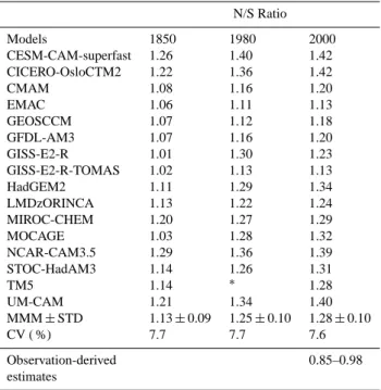
Table 2. Inter-hemispheric ratio (N/S) of tropospheric mean OH from models for 1850, 1980 and 2000 time-slices. Observation-derived estimates shown in the last row are based on Montzka et al. (2001), Prinn et al. (2001), Krol and Lelieveld (2003), and Bous-quet et al. (2005). A cell with∗means that the model did not report that quantity N/S Ratio Models 1850 1980 2000 CESM-CAM-superfast 1.26 1.40 1.42 CICERO-OsloCTM2 1.22 1.36 1.42 CMAM 1.08 1.16 1.20 EMAC 1.06 1.11 1.13 GEOSCCM 1.07 1.12 1.18 GFDL-AM3 1.07 1.16 1.20 GISS-E2-R 1.01 1.30 1.23 GISS-E2-R-TOMAS 1.02 1.13 1.13 HadGEM2 1.11 1.29 1.34 LMDzORINCA 1.13 1.22 1.24 MIROC-CHEM 1.20 1.27 1.29 MOCAGE 1.03 1.28 1.32 NCAR-CAM3.5 1.29 1.36 1.39 STOC-HadAM3 1.14 1.26 1.31 TM5 1.14 ∗ 1.28 UM-CAM 1.21 1.34 1.40 MMM ± STD 1.13 ± 0.09 1.25 ± 0.10 1.28 ± 0.10 CV ( %) 7.7 7.7 7.6 Observation-derived 0.85–0.98 estimates

the small stratospheric and oceanic losses (Prinn et al., 2005; Prather et al., 2012).

3 Historical OH and methane lifetime

Table 1 shows annual mean global total methane burden, tropospheric mean OH and methane lifetime from the 16 global models for the 1850, 1980 and 2000 time-slices. The global methane burden increases by more than a factor of two from 1850 to 2000 in all models. Simulated methane abundances are not sensitive to how methane was prescribed in the models (Lamarque et al., 2013). Despite similar im-posed changes in emissions, specifically increases in the emissions of NOx (contributing to secondary OH

produc-tion), CO and NMVOCs (OH sinks) (Young et al., 2013), and in the methane burden over the 1850 to 2000 period, the models simulate different change in OH ranging from an increase to a decrease. All models simulate larger increases or smaller decreases in tropospheric OH abundance in the Northern Hemisphere (NH) compared to the Southern Hemi-sphere (SH) consistently from 1850 to 2000 (Table 2). We ex-plore the changes in OH, methane lifetime and their driving factors for present-day relative to preindustrial and to 1980 in Sects. 4 and 5, respectively, in an attempt to identify the key processes responsible for the different simulated OH trends.

3.1 Evaluation of present-day OH

Comparison between modeled and observed OH concentra-tions provides insight into the budget of OH and an un-derstanding of the underlying chemistry (e.g. Stone et al., 2012 and references therein). A thorough evaluation of mod-els against direct OH measurements (ground-based, aircraft) is not particularly useful for constraining global mean OH because of the enormous temporal and spatial variability in OH concentrations. Since our simulations represent average climatological conditions, we focus our evaluation on some of the factors controlling OH distributions at regional and global scales.

Lifetimes of methane and CH3CCl3against reaction with

tropospheric OH provide the best constraints on the global mean tropospheric OH concentration. We compare present-day (2000) methane and CH3CCl3 lifetimes obtained from

models against observationally derived estimates to evalu-ate the global mean OH concentrations simulevalu-ated by the models. The multi-model mean methane lifetime against OH loss of 9.7 ± 1.51 years (Table 1) is about 5 % lower than the mean 1978–2004 tropospheric methane lifetime of 10.2+0.9_−0.7yr estimated by Prinn et al. (2005), and is about 13 % lower than the most up-to-date observationally derived estimate of 11.2 ± 1.3 yr for 2010 (Prather et al., 2012). It is identical to the methane lifetime of 9.7 ± 1.7 yr ob-tained from a previous multi-model analysis (Shindell et al., 2006b), and is about 5 % lower than the 10.2 ± 1.7 yr reported in the recent Hemispheric Transport of Air Pol-lution (HTAP) multi-model study (Fiore et al., 2009). The variation in methane lifetime across participating models is about the same as that across the previous multi-model esti-mates (Shindell et al., 2006b; Fiore et al., 2009). Similarly, the multi-model mean CH3CCl3lifetime of 5.7 ± 0.9 yr

(Ta-ble 1), is about 5 % lower than the observationally derived tropospheric lifetime of 6.0+0.5_−0.4years over the period 1978– 2004 (Prinn et al., 2005), and is about 10 % lower than the recent estimate of 6.3 ± 0.4 years (Prather et al., 2012) ob-tained using CH3CCl3 observations over the period 1998–

2007 (Montzka et al., 2011). This comparison suggests that the multi-model mean present-day global tropospheric OH abundance of 11.1 ± 1.6 × 105molec cm−3is overestimated by 5 to 10 % but is within the uncertainty range of observa-tions.

Since the atmospheric oxidizing capacity is sensitive to both the OH amount and its spatial distribution (Lawrence et al., 2000), we examine the regional OH distribution in the models as depicted in Fig. 1a showing the multi-model mean OH concentrations in the different atmospheric sub-domains for the 2000 time-slice (individual models are shown in Fig. S1 in the Supplement). Consistent with previous studies,

1_{Slightly different from that reported by Voulgarakis et} al. (2013) as we have included results from GISS-E2-R-TOMAS and TM5.

(8)

54

Figure 1. a) Multi-model mean regional annual mean airmass-weighted OH concentrations (x105_{molecule cm}-3_{) and b) the coefficient of variation (CV; standard deviation as percentage of} the multi-model mean) for 2000 in the atmospheric subdomains recommended by Lawrence et al. (2001). Global mean tropospheric OH concentration and CV are shown in the topmost row of each plot.

Fig. 1. (a) Multi-model mean regional annual mean airmass-weighted OH concentrations (× 105 molecule cm−3) and (b) the coefficient of variation (CV; standard deviation as percentage of the multi-model mean) for 2000 in the atmospheric subdomains recom-mended by Lawrence et al. (2001). Global mean tropospheric OH concentration and CV are shown in the topmost row of each plot.

the greatest OH concentrations are found in the tropical tro-posphere reflecting the abundant sunlight and water vapor (Fig 1a). The individual model biases in tropical specific humidity compared with reanalysis and satellite measure-ments (Lamarque et al., 2013) are generally consistent with OH concentrations in the tropical troposphere, i.e., models with high water vapor biases simulate high OH (compare Figs. S1 with S4 of Lamarque et al., 2013). The NH ex-tratropical troposphere is characterized by higher OH con-centrations than that in the SH extra-tropics reflecting the influence of higher ozone and NOx emissions. A

compari-son of present-day model tropospheric ozone concentrations against ozonesonde and satellite data indicates that models may have a systematic high bias in the extratropical NH (Young et al., 2013) perhaps contributing to the high NH extratropical OH. The larger model overestimate of the to-tal column ozone (mainly reflecting stratospheric ozone col-umn) relative to satellite measurements from the merged To-tal Ozone Mapping Spectrometer/solar backscatter ultravio-let (TOMS/SBUV) data averaged over the 1996–2005 time period (Fig. S2) in the SH than in the NH may also con-tribute to lower simulated OH concentrations in the extrat-ropical SH.

Overall, there is large model-to-model variability in the regional distribution of OH. There is, however, less inter-model diversity in the mid-troposphere OH concentrations compared with those in the lower and upper troposphere (Fig. 1b), except in the SH troposphere where the large inter-model variation possibly reflects diversity in the simulated stratospheric ozone columns and differences in how these influence photolysis in the models. Clouds have also been shown to influence the regional distribution of OH via pho-tolysis (Liu et al., 2006; Voulgarakis et al., 2009). Evalua-tion of parent climate models of many of the ACCMIP mod-els against “A-Train” satellite observations indicates that wa-ter vapor and clouds are simulated betwa-ter in the lower and middle troposphere than in the upper troposphere (Jiang et al., 2012) – a factor possibly contributing to the large

uncer-tainty in upper tropospheric OH concentrations. An exhaus-tive evaluation of the regional distributions of OH requires more process-level information from the models (e.g. OH production and loss fluxes, and cloud properties) and should be a priority for future model inter-comparisons.

The present-day multi-model mean OH inter-hemispheric (N/S) ratio is 1.28 ± 0.1 (Table 2), in contrast to the range of N/S values derived from measurements of CH3CCl3

encom-passing the 1980 to 2000 period (Montzka et al., 2000; Prinn et al., 2001; Krol and Lelieveld, 2003; Bousquet et al., 2005). For example, with CH3CCl3measurements for 1998–1999,

Montzka et al. (2000) estimate that annual mean OH con-centrations are 15 ± 10 % higher south of the inter-tropical convergence zone (ITCZ) than north of it, while Prinn et al. (2001) derive annual mean OH concentrations that are 14 ± 35 % higher in the SH than the NH over the 1978–2000 time period. These observational estimates of N/S OH ratio are highly uncertain as they rely on the assumption of accu-rate CH3CCl3emission estimates and its atmospheric

obser-vations. Nevertheless, model derived N/S inter-hemispheric asymmetry is consistent with present-day tropospheric ozone distributions in the ACCMIP models that are biased high and low in the NH and SH, respectively, against satellite and ozonesonde observations (Young et al., 2013). The models thus overestimate OH production from ozone in the NH rel-ative to SH.

Several factors including model-to-model differences in emissions, particularly natural emissions (since models used similar anthropogenic emissions), underlying chemi-cal mechanisms (that dictate the VOC speciation and emis-sions), stratospheric ozone column, cloud amounts, photol-ysis schemes, and interactions with aerosols likely all con-tribute to the large intermodel variation in the simulated present-day tropospheric OH concentrations (and methane and CH3CCl3 lifetimes). For example, lowest tropospheric

mean OH in UM-CAM most likely stems from its offline photolysis scheme that does not account for changes in clouds, overhead ozone column, or aerosols, resulting in very low photolysis rates and OH (Voulgarakis et al., 2013). The highest tropospheric mean OH abundances are simu-lated by the CESM-CAM-superfast and MOCAGE models. The representation of NMVOCs is minimal in CESM-CAM-superfast model as it includes isoprene only, thus simulat-ing a smaller sink for OH. Even though MOCAGE has the highest NMVOC emissions, thus a bigger OH sink, (Ta-ble S1), other factors contribute to its high OH, including the lack of inclusion of aerosol photochemical effects in the model (Bousserez et al., 2007). In addition, low strato-spheric ozone columns in MOCAGE may enhance UV radi-ation resulting in greater OH production, although we cannot directly diagnose this as photolysis rates are not available from MOCAGE. High NMVOC emissions have also been suggested as a possible reason for high OH in MOCAGE (Voulgarakis et al., 2013). Availability of key OH diag-nostics from all models participating in future multi-model

(9)

55

Figure 2. Annual average bias of multi-model mean CO for 2000 against a) surface CO observations averaged over the 1996 to 2005 period from the NOAA Global Monitoring Division (GMD) network (Novelli and Masarie, 2010; downloaded on April 11, 2012) and b) average 2000-2006 MOPITT CO at 500 hPa. Each circle in (a) indicates the annual mean bias at the CO measurement site. For comparison with satellite observations in (b), each model was convolved with the MOPITT operator (a priori and averaging kernels) before taking the difference.

a

b

Fig. 2. Annual average bias of multi-model mean CO for 2000 against (a) surface CO observations averaged over the 1996–2005 period from the NOAA Global Monitoring Division (GMD) net-work (Novelli and Masarie, 2010; downloaded on April 11, 2012) and (b) average 2000–2006 MOPITT CO at 500 hPa. Each circle in (a) indicates the annual mean bias at the CO measurement site. For comparison with satellite observations in (b), each model was con-volved with the MOPITT operator (a priori and averaging kernels) before taking the difference.

intercomparison projects will facilitate a better understand-ing of inter-model diversity in OH distributions and con-tribute to a process-based understanding of the drivers of OH.

3.2 Comparison of present-day CO with observations

CO is the major sink of tropospheric OH (Jacob 1999; Dun-can and Logan, 2008), hence, any biases in CO will likely influence the distribution of OH. Here, we evaluate the simu-lated CO distributions against surface and satellite measure-ments to test if OH sinks may also be too low in the NH com-pared with the SH resulting in higher NH-OH concentrations. We compare annual mean CO from the models with sur-face CO measurements averaged over the 1996–2005 period from the NOAA Global monitoring Division (GMD) Carbon Cycle Cooperative Global Air Sampling Network (Novelli and Masarie, 2010) for 50 sites (Fig. 2a) and with the ob-served mean 2000–2006 CO distribution at 500 hPa from the Measurements of Pollution In The Troposphere (MOPITT) instrument (Fig. 2b). For comparison with surface observa-tions, we sampled model results at pressure levels closest

to the pressure altitude, latitude and longitude of the ob-servation sites. For comparison with MOPITT CO, we used monthly mean daytime values derived from version 4 (V4) level 3 retrievals from March 2000 to December 2006 pro-vided at a horizontal resolution of 1◦×1◦and at 10 retrieval levels (Deeter et al., 2010). For proper comparison, we trans-formed each model’s CO by first interpolating it to the MO-PITT grid and then applying the averaging kernel and a pri-ori profile associated with each MOPITT retrieval (Shindell et al., 2006b; Emmons et al., 2009). A priori profiles associ-ated with V4 are based on a monthly climatology from the global chemical transport model MOZART-4. Detailed eval-uation of MOPITT V4 CO retrievals between 2002 and 2007 with in situ measurements show biases of less than 1 % at the surface, 700 hPa and 100 hPa, and a bias of about −6 % at 400 hPa (Deeter et al., 2010).

The multi-model mean underestimates the observed sur-face CO concentrations at most sites in the NH (Fig. 2a), with strong negative biases (up to 60 ppbv) at many high latitude sites. Negative biases persist at the northern mid-latitude sites albeit with smaller magnitudes than at the northern high-latitude sites. In the SH, the multi-model mean is within

±2 ppbv at most sites. Consistent with the surface CO com-parison, the multi-model mean underestimates the MOPITT CO at 500 hPa throughout the NH, except over northern In-dia and south-central China (Fig. 2b). The overestimate over these South Asian regions is present in all models (Fig. S3) and is particularly dominant in the comparison for Septem-ber (not shown), indicating excessive transport and/or emis-sions. The multi-model mean CO reproduces the MOPITT values over much of the SH, except over central Africa, west-ern South America, Indonesia and surrounding Indian and Pacific oceans possibly related to discrepancies in biomass burning emissions (Fig 2b). Despite these regional biases, the models capture the overall spatial distribution of MOPITT CO fairly well as indicated by the high values of spatial cor-relation coefficients (Table 3).

The multi-model mean CO concentrations generally agree better with observations in the SH, and are biased low in the NH, similar to the earlier multi-model results of Shindell et al. (2006b). The simulated low CO levels in the NH are con-sistent with a weaker-than-observed OH sink that contributes to the larger OH north-to-south asymmetry compared to that derived from CH3CCl3observations.

4 Preindustrial to present-day changes in OH and methane lifetime, and their driving factors

We now explore the changes in OH from preindustrial to present-day and their driving factors. The multi-model tro-pospheric mean OH oxidative capacity has remained nearly constant over the past 150 yr (Table 4). Globally, increases in factors that enhance OH – humidity (4.7 ± 2.6 %), tropo-spheric ozone (38 ± 10.8 %; Young et al., 2013) and NOx

(10)

Table 3. Model versus MOPITT CO annual mean bias for the Northern Hemisphere (NH), Southern Hemisphere (SH), and Global at 500 hPa. Annual mean spatial pattern correlation coefficients (r) between model and MOPITT CO global retrievals are in the right-most column.

Bias (ppbv) Models NH SH Global r CESM-CAM-superfast −31.92 −17.65 −24.79 0.83 CICERO-OsloCTM2 1.56 6.99 4.28 0.86 CMAM −13.68 −4.54 −9.10 0.93 EMAC −1.79 2.24 0.23 0.93 GEOSCCM −5.73 0.00 −2.86 0.87 GFDL-AM3 −9.01 0.58 −4.22 0.89 GISS-E2-R 19.23 25.64 22.43 0.91 GISS-E2-R-TOMAS 7.54 11.88 9.71 0.89 HadGEM2 3.05 6.40 4.73 0.76 LMDzORINCA 3.14 4.36 3.75 0.93 MIROC−CHEM −12.57 −0.76 −6.65 0.92 MOCAGE 0.67 −2.46 −0.89 0.76 NCAR−CAM3.5 −12.59 −0.05 −6.32 0.87 STOC−HadAM3 7.37 11.22 9.31 0.85 TM5 −10.27 −1.33 −5.80 0.86 UM-CAM 13.24 21.27 17.26 0.89 MMM ± STD −2.6 ± 12.4 4.0 ± 10.3 0.7 ± 11.2 0.87 ± 0.05

Table 4. Preindustrial (1850) to present-day (2000) changes in global mean tropospheric OH, tropospheric methane lifetime (τ_CH4), CO and NOxburdens, stratospheric ozone column (Strat O3), humidity (Q), and temperature (T ). Absolute changes in airmass-weighted temperature are given, while the rest of the quantities are expressed as percentage changes relative to 1850. Models that simulate reductions in present-day OH relative to preindustrial are shown in bold. A cell with∗means that the model did not report that quantity.

Models 1OH (%) 1τCH4(%) 1CO (%) 1NOx(%) 1Strat O3(%) 1Q (%) 1T (K) CESM-CAM-superfast 6.1 −9.8 100.3 243.8 −7.6 8.1 1.4 CICERO-OsloCTM2 −11.1 9.2 114.3 89.8 0.5 0.0 0.0 CMAM −9.6 8.1 110.9 56.3 −3.2 8.3 1.2 EMAC −7.6 2.1 102.1 63.4 −1.2 5.4 0.9 GEOSCCM −12.7 12.0 120.3 62.5 −4.0 5.7 1.0 GFDL-AM3 −8.1 5.1 86.1 41.8 −2.4 3.4 0.6 GISS-E2-R 7.0 −10.6 68.9 39.5 −6.1 5.8 0.9 GISS-E2-R-TOMAS 9.1 −11.7 71.1 33.6 −6.6 7.6 1.1 HadGEM2 −0.7 −0.1 84.3 192.5 −6.0 3.3 0.5 LMDzORINCA −5.9 4.1 94.8 87.0 0.3 ∗ 0.8 MIROC-CHEM −7.3 ∗ 100.9 75.9 −3.1 4.7 0.8 MOCAGE 14.6 −13.5 58.1 286.6 −19.7 5.2 0.9 NCAR-CAM3.5 11.7 −14.1 66.3 114.7 −3.3 6.9 1.1 STOC-HadAM3 3.2 −5.7 71.1 111.0 −4.0 3.5 0.6 TM5 −4.3 1.2 94.1 67.7 0.6 0.0 0.0 UM-CAM 6.0 −6.7 81.9 161.6 −6.1 3.5 0.6 MMM ± STD −0.6 ± 8.8 −2.0 ± 8.8 89.1 ± 18.6 108.0 ± 75.4 −4.5 ± 4.8 4.7 ± 2.6 0.8 ± 0.4

(as NO + NO2) burdens (108.0 ± 75.4 %), and decreases

in stratospheric ozone (−4.5 ± 4.8 %), which modulate tro-pospheric ozone photolysis rates – are compensated by in-creases in OH sinks – doubling of methane (Table 1) and CO burdens (Table 4). Tropospheric temperature that con-trols water vapour abundance and reaction rates also in-creases (0.8 ± 0.4 K) during this period. The near-constant global mean OH over the historical period is consistent with

the findings of Lelieveld et al. (2002, 2004). There is, how-ever, large intermodel spread in the simulated changes in OH, ranging from a decrease of 12.7 % (GEOSCCM) to an in-crease of 14.6 % (MOCAGE) (Table 4). It is notable that with the consistent ACCMIP modeling specifications, the preindustrial to present-day percent changes in OH for all ACCMIP models are within ± 15 %, a range significantly reduced from the previously published model estimates of

(11)

preindustrial to present-day OH changes (Table 1 of John et al., 2012).

We now discuss regional changes in annual mean OH by relating them to regional changes in chemistry (CO, NOx

burdens, stratospheric ozone) and climate drivers (humidity and temperature) of OH. Preindustrial to present-day changes in multi-model mean OH, CO and NOx burdens, humidity

and temperature for 12 tropospheric subdomains, as defined by Lawrence et al. (2001), are shown in Fig. 3 (left col-umn). Strong intermodel diversity exists in the magnitude of NOx burden changes, particularly in the upper troposphere

(Fig. 3e), possibly reflecting the model-to-model differences in processes that dominate the response in this region and the uncertainty associated with lightning NOx emissions.

The intermodel diversity in CO, humidity and temperature changes is much lower compared to that for NOxchanges.

Strong intermodel variation exists in both the sign and mag-nitude of regional preindustrial to present-day changes in OH (see Fig. S4 for regional OH changes in individual mod-els). For many atmospheric regions, the standard deviation in OH change across models is greater than the multi-model mean change (Fig. 3a) suggesting that the changes are not statistically significant. The NH lower tropospheric (surface to 750 hPa) extra-tropics (30◦–90◦N) is the only region of the atmosphere where the models agree on the sign of OH change (increase), and its magnitude appears to be statisti-cally significant (multi-model mean greater than standard de-viation). This is also the region with the largest increases in CO and NOxburdens (Fig. 3c, e), driven by the changes in

anthropogenic emissions which are similar in all the models. Humidity levels increase everywhere (Fig. 3g) in response to temperature increases (Fig. 3i). Strong increases in tro-pospheric ozone, the primary source of OH, are also simu-lated in the NH lower troposphere in response to emission increases (Young et al., 2013). Thus, combined increases in water vapor, ozone and NOxoutweigh CO increases resulting

in enhanced OH levels in the NH extratropical lower tropo-sphere in the present-day relative to preindustrial.

Reflecting the changes in OH, there is a large in-termodel variability in the preindustrial to present-day change in methane lifetime (Table 4) with increase of 12 % (GEOSCCM) to decrease of 14.1 % (NCAR-CAM3.5). Changes in methane lifetime for each model are inversely proportional to the OH change in the model, except for HadGEM2 which shows no change in global mean OH.

4.1 Diversity in preindustrial to present-day changes

Here, we explore the diversity in preindustrial to present-day changes in global OH using the ratio of the change in global mean tropospheric CO and NOx burdens (1CO/1NOx

-approximately represents changes in OH sinks versus changes in OH sources) simulated by the models. Previous studies have found a linear dependence of changes in global mean OH to the ratio of CO and hydrocarbon sources and

Fig. 3. Multi-model mean percentage change in tropospheric OH, CO and NOxburdens, humidity (Q), and absolute change in temper-ature for 12 subdomains of the atmosphere as defined by Lawrence et al. (2001) for 2000–1850 (left) and 2000–1980 (right). Decreases are shown in red and increases are in black. Changes in the mean global (Glob), Southern Hemisphere (SH), and Northern Hemi-sphere (NH) tropoHemi-sphere (surface to 200 hPa) are shown in the top-most row of each plot.

NOx sources (Wang and Jacob, 1998) or to the ratio of CO

and NOx emissions when changes in VOC emissions are

small (Dalsøren and Isaksen, 2006). We find that intermodel variation in the sign and magnitude of the preindustrial to present-day change in global mean OH, whether positive or negative, correlates strongly with 1CO/1NOx (Fig. 4;

coefficient of determination (r2) =0.7). Models that sim-ulate decreases in present-day global mean OH relative to

(12)

58

Figure 4. Scatterplot of absolute change in annual average tropospheric mean OH concentration

from preindustrial (1850) to present day (2000) versus the ratio of absolute changes in annual average total tropospheric CO and NOx burdens for each of the 16 models. Each model data

point is denoted by the first two letters of the model name shown in Table 1. Solid line corresponds to a linear regression of changes in OH with the ratio of changes in CO and NOx

burdens. The regression equation is shown on the upper right corner of the plot.

Fig. 4. Scatterplot of absolute change in annual average tro-pospheric mean OH concentration from preindustrial (1850) to present-day (2000) versus the ratio of absolute changes in annual average total tropospheric CO and NOxburdens for each of the 16 models. Each model data point is denoted by the first two letters of the model name shown in Table 1. Solid line corresponds to a linear regression of changes in OH with the ratio of changes in CO and NOxburdens. The regression equation is shown on the upper right corner of the plot.

preindustrial have stronger increases in OH sinks compared with sources (except HadGEM2), while models that simu-late increase in OH show larger relative increases in sources versus sinks (except GISS-E2-R and GISS-E2-R-TOMAS) (Table 4). Removing the three outlier models increases the

r2to 0.8. The correlation is particularly tight for models that simulate preindustrial to present-day OH decreases.

This analysis leads to the question of why the preindus-trial to present-day changes in global CO and NOxburdens

are different across models despite imposing seemingly sim-ilar trends in total CO and NOxemissions and methane

bur-dens (Fig. 1 and Table S1 of Young et al., 2013). We attribute the diversity in 1CO/1NOxto differences in emissions and

chemical schemes implemented in the models. The variation in the simulated preindustrial to present-day methane bur-den trends is small (Table 1), however there are large dif-ferences in the CO, NOxand NMVOC emission trends

(Ta-ble S4) as implemented in the models that drive differences in 1CO/1NOx, and therefore, OH. Variation in CO and NOx

emissions is due to differences in natural emissions (CO from oceans and vegetation; NOxfrom soils and lightning) (Young

et al., 2013). Additional spread in CO source strength is due to the complexity of NMVOC chemical mechanism included in the models (Young et al., 2013), since NMVOC oxida-tion is a major CO source (Holloway et al., 2000; Duncan et al., 2007; Grant et al., 2010). For example, some mod-els with simpler NMVOC chemistry include extra CO emis-sions to account for missing NMVOCs (see Table A1). Dif-ferent NMVOC oxidation mechanisms lead to a wide range in both anthropogenic (prescribed mostly from the inventory

of Lamarque et al., 2010) and biogenic NMVOC emissions. Additional diversity in biogenic NMVOC emission trends comes from the different ways these (particularly isoprene as it is the dominant biogenic NMVOC) are specified (con-stant versus climate-sensitive) in the models (Table A1). Fur-thermore, even if the total emissions were identical across models, differences in the way the physical processes (for example, depositional loss, photolysis) that influence the at-mospheric lifetimes of CO and NOxin the models will likely

produce differences in their atmospheric distributions and trends. Thus, uncertainties in natural emissions and differ-ences in chemical and physical processes implemented in the models drive the spread in the interplay between OH sources and sinks (approximated as 1CO/1NOx) resulting in the

di-versity in preindustrial to present-day OH changes.

Better constraints on natural emissions and the key physi-cal processes controlling the distribution of OH sources and sinks will help advance our understanding of the evolution of atmospheric OH. Furthermore, concerted efforts to evalu-ate tropospheric chemistry mechanisms implemented in the models (Luecken et al., 2008; Emmerson and Evans, 2009; Archibald et al., 2010; Chen et al., 2010; Barkley et al., 2011) will also help to make progress in understanding the diversity in OH distributions and long-term trends across the current generation of chemistry-climate models.

5 1980 to 2000 changes in OH and methane lifetime

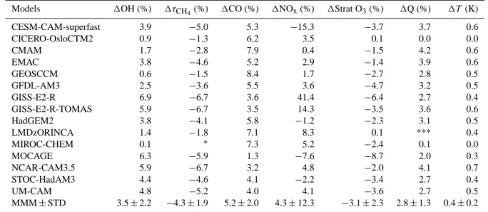
We now explore the change in OH and methane lifetime over the 1980 to 2000 period. Consistent with prior modeling studies (Karlsd´ottir and Isaksen, 2000; Dentener et al., 2003; Dalsøren and Isaksen, 2006; Hess and Mahowald, 2009; John et al., 2012; Holmes et al., 2013), the multi-model mean OH increases slightly from 1980 to 2000 by 3.5 ± 2.2 % (Ta-ble 5). Over this period, increases in OH sinks, specifically the methane (12 ± 1.9 %) and CO (5.2 ± 2.0 %) burdens are slightly outweighed by increases in humidity (2.8 ± 1.3 %), NOx burdens (4.3 ± 12.3 %), and stratospheric ozone loss

(3.1 ± 2.3 %). In contrast to the disagreement in the sign of OH change for the 1850–2000 period, all models agree on a small OH increase from 1980 to 2000. The multi-model mean methane lifetime decreases by 4.3 ± 1.9 % from 1980 to 2000 reflecting the small increase in tropospheric OH and warming of 0.4 ± 0.2 K. While the models are consis-tent with each other, the observational estimates of trends in OH derived from CH3CCl3measurements indicate a ∼10 %

decrease over a similar period (Prinn et al., 2001; Bousquet et al., 2005). More recent analysis of CH3CCl3observations

over the 1998–2007 period indicates that global OH is well buffered against perturbations (Montzka et al., 2011) and suggests that the uncertainties in CH3CCl3data before 1998

may have led to artificially large OH trends reported in previ-ous studies. Better constraints on OH trends are important for

(13)

inferring trends in methane sources (and other species lost by OH) via inverse methods.

Regionally, the NH shows larger OH increases

(4.6 ± 1.9 %) (Fig. 3b) than the SH (2.2 ± 3.2 %), the latter being where intermodel variability is large (Fig. S5). The largest increases occur in the NH extratropical tropo-sphere (Fig. 3b), which coincide with increases in humidity (Fig. 3h), and decreases in the CO burden (Fig. 3f). NOx

burdens decrease in the extratropical NH lower troposphere in 2000 relative to 1980, possibly driven by decreasing North American and European emissions (Lamarque et al., 2010; Granier et al., 2011). The large intermodel diversity in the sign of change in the SH may be related to the extent of stratospheric ozone loss and its influence on photolysis as simulated by the models. Previous studies have identified the stratospheric ozone column through its influence on photolysis as a key driver of trends and variability in tropo-spheric OH, particularly in the SH (Dentener et al., 2003; Wang et al., 2004). Anecdotally, models that simulate strong stratospheric ozone losses and allow the ozone column to affect photolysis rates simulate stronger OH increases (e.g., GISS-E2-R and MOCAGE), particularly in the extratropical troposphere. Sensitivity simulations that isolate the role of changes in emissions, overhead ozone column, and meteo-rology are needed to explain the OH trends and intermodel diversity over the 1980–2000 period (e.g., Dentener et al., 2003).

6 Sensitivity of OH and methane lifetime to climate

We investigate the influence of climate change on OH and methane lifetime by analysing the simulations performed by 10 models with 2000 emissions but driven by 1850s climate (Em2000Cl1850). We compare the base 2000 time-slice and Em2000Cl1850 simulations to diagnose the impact of cli-mate change from 1850 to 2000.

Preindustrial to present-day climate change causes a multi-model mean global OH increase of 2.1 ± 2.0 % (Fig. 5) and a methane lifetime decrease of 0.30 ± 0.24 yr (Table 6). All models, except GFDL-AM3, simulate OH increases (Fig. 5) and methane lifetime decreases (Table 6) in response to his-torical climate change. GISS-E2-R produces the strongest methane lifetime decrease, while STOC-HadAM3 produces the strongest methane lifetime decrease per unit tempera-ture increase. Increases in water vapour cause tropospheric OH increases, particularly in the upper troposphere where the relative increases in humidity (Fig. 6a) are greatest. Warmer temperatures and increased OH enhance oxidative loss of methane (Fig. 6c), decreasing the methane lifetime by 0.30 ± 0.24 yr (Table 6) and representing a small negative climate feedback, in agreement with prior studies (Steven-son et al., 2000, 2006; John(Steven-son et al., 2001; Voulgarakis et al., 2013).

59

Figure 5. Percent tropospheric mean OH concentration change due to preindustrial to present day changes in climate (Em2000Cl1850), methane burden (Em2000CH41850), and anthropogenic emissions of CO (Em2000CO1850), NOx, (Em2000NOx1850), and NMVOCs

(Em2000NMVOC1850). The multi-model mean (MMM) OH changes for each experiment are also shown.

Fig. 5. Percent tropospheric mean OH concentration change due to preindustrial to present-day changes in climate (Em2000Cl1850), methane burden (Em2000CH41850), and anthropogenic emis-sions of CO (Em2000CO1850), NOx, (Em2000NOx1850), and NMVOCs (Em2000NMVOC1850). The multi-model mean (MMM) OH changes for each experiment are also shown.

7 Attribution of OH changes to methane burden and NOx, CO, and NMVOC emissions

A subset of the models performed a series of attribution experiments with 2000 climate conditions but with anthro-pogenic CO, NOxand NMVOC emissions, and methane

con-centrations individually set to preindustrial levels. For the methane attribution experiment performed by eight models (Em2000CH41850), the methane concentration was fixed at an 1850s level (791 ppbv), while for the emissions attribu-tion experiments (Em2000CO1850, Em2000NOx1850, and Em2000NMVOC1850) conducted by six models, methane was fixed at a 2000s level (1751 ppbv) and anthropogenic emissions were reduced to their 1850 values separately for each simulation. We subtract results of each perturbation simulation from the base 2000 time-slice simulation to diag-nose the impact of preindustrial (1850) to present-day (2000) changes in each of the specific drivers on OH, as shown in Fig. 5. Because methane concentrations were prescribed (rather than using emissions), these attribution simulations are not at steady state with respect to methane concentra-tion and, therefore, OH (Prather, 1994, 1996; Fuglestvedt et al., 1999; Derwent et al., 2001; Wild et al., 2001; Stevenson et al., 2004; Naik et al., 2005; Shindell et al., 2005, 2009; West et al., 2007; Fiore et al., 2008). Here, we only diag-nose instantaneous changes in methane lifetime; steady-state changes are addressed by Stevenson et al. (2013).

The largest change in global mean OH is simulated for preindustrial to present-day increases in anthropogenic NOx

emissions, followed by increases in methane concentrations, while smaller changes result from increases in CO and NMVOCs emissions across the subset of models (Fig. 5). Global mean OH increases by 46.4 ± 12.2 % due to NOx

(14)

Table 5. Same as in Table 4 but for changes in present-day (2000) relative to 1980.

Models 1OH (%) 1τCH4(%) 1CO (%) 1NOx(%) 1Strat O3(%) 1Q (%) 1T (K) CESM-CAM-superfast 3.9 −5.0 5.3 −15.3 −3.7 3.7 0.6 CICERO-OsloCTM2 0.9 −1.3 6.2 3.5 0.1 0.0 0.0 CMAM 1.7 −2.8 7.9 0.4 −1.5 4.2 0.6 EMAC 3.8 −4.6 5.2 2.9 −1.4 3.9 0.6 GEOSCCM 0.6 −1.5 8.4 1.7 −2.7 2.8 0.5 GFDL-AM3 2.5 −3.6 5.5 3.6 −4.7 3.2 0.5 GISS-E2-R 6.9 −6.7 3.6 41.4 −6.4 2.7 0.4 GISS-E2-R-TOMAS 5.9 −6.7 3.5 14.3 −3.5 3.6 0.6 HadGEM2 3.8 −4.1 5.8 −1.2 −2.3 3.1 0.5 LMDzORINCA 1.4 −1.8 7.1 8.3 0.1 *** 0.4 MIROC-CHEM 0.1 ∗ 7.3 5.2 −2.4 0.1 0.0 MOCAGE 6.3 −5.9 1.3 −7.6 −8.7 2.0 0.3 NCAR-CAM3.5 5.9 −6.7 3.2 4.8 −2.0 4.1 0.7 STOC-HadAM3 4.4 −4.6 4.1 −2.2 −3.4 2.7 0.4 UM-CAM 4.8 −5.2 4.0 4.1 −3.6 2.7 0.5 MMM ± STD 3.5 ± 2.2 −4.3 ± 1.9 5.2 ± 2.0 4.3 ± 12.3 −3.1 ± 2.3 2.8 ± 1.3 0.4 ± 0.2

Table 6. Change in tropospheric methane lifetime (τCH4) due to climate change: difference between base 2000 time-slice and a simula-tion with 1850 climate (Em2000Cl1850). Change in tropospheric temperature (1T ) and lifetime change per unit change in temperature (1τ_CH4/1T ) are also shown for 10 models.

Models 1τCH4 (years) 1T (K) 1τCH4/1T (yr K −1₎ CESM-CAM-superfast −0.27 1.4 −0.20 GFDL-AM3 0.12 0.6 0.21 GIS-E2-R −0.76 1.1* −0.69 GISS-E2-R-TOMAS −0.70 1.1 −0.64 HadGEM2 −0.20 0.5 −0.40 MIROC-CHEM −0.25 0.8 −0.30 MOCAGE −0.20 0.9 −0.23 NCAR-CAM3.5 −0.37 1.1 −0.34 STOC-HadAM3 −0.46 0.6 −0.71 UM-CAM −0.34 0.6 −0.55 MMM ± STD −0.30 ± 0.24 0.9 ± 0.3 −0.39 ± 0.28

∗_{Temperature change is slightly different from that reported in Table 4 as a different base simulation}

was used to compare the Em2000Cl1850 simulation.

emission increases as a result of increases in both primary and secondary OH production. The more than a factor of two increases in methane concentrations at present-day NOx

levels leads to increases in tropospheric ozone, the primary source of OH. However, OH is consumed during the oxida-tion of methane and its oxidaoxida-tion products, so that the net result is a global OH decrease of 17.3 ± 2.3 %. Smaller de-creases in mean OH occur in response to anthropogenic CO (7.6 ± 1.5 %) and NMVOC emission (3.1 ± 3.0 %) increases (Fig. 7). Despite being the major OH sink, the decrease in OH from CO increase is smaller than that from methane in-crease because of the lack of additional oxidation products that can further consume OH.

Methane lifetime also responds most strongly to in-creases in NOx, followed by methane, CO and NMVOC,

respectively. However, the response in the perturbation life-time is different when the nonlinear feedback of methane on its own lifetime is considered (Stevenson et al., 2013). Fur-thermore, the sum of OH or methane lifetime changes diag-nosed from the individual attribution experiments performed by a model is not equal to the total preindustrial to present-day diagnosed from the historical time-slice simulations (Ta-ble 4). This is partly because of the inherent nonlinear chem-ical system and partly because all the offsetting processes influencing OH in the coupled chemistry-climate system are not included in these attribution experiments.

Regionally, OH reductions are slightly stronger in the SH compared with the NH in response to methane changes (Fig. 7a) since methane is a more important OH sink in the SH than in NH (Spivakovsky et al., 2000). On the other

(15)

60

Figure 6. Percent change in multi-model mean (10 models) regional a) specific humidity, b)

tropospheric OH and c) methane loss flux due to climate change only (2000-Em2000Cl1850). Decreases are shown in red and increases are in black.

Fig. 6. Percent change in multi-model mean (10 models) regional a) specific humidity, b) tropospheric OH and c) methane loss flux due to climate change only (2000–Em2000Cl1850). Decreases are shown in red and increases are in black.

61

Figure 7. Percent change in multi-model mean OH in 12 subdomains of the atmosphere for 2000 relative to attribution experiments: a) Em2000CH41850 (8 models), b) Em2000CO1850 (6 models), c) Em2000NOx1850 (6 models), d) Em2000NMVOC1850 (6 models). OH increases are shown in black and decreases are in red.

Fig. 7. Percent change in multi-model mean OH in 12 subdomains of the atmosphere for 2000 relative to attribution experiments: a) Em2000CH41850 (8 models), b) Em2000CO1850 (6 models), c) Em2000NOx1850 (6 models), d) Em2000NMVOC1850 (6 mod-els). OH increases are shown in black and decreases are in red.

hand, OH decreases are stronger in the NH compared with SH for CO and NMVOC emission increases (Fig. 7b, d), re-flecting higher anthropogenic sources in the NH and shorter lifetimes. Increases in anthropogenic NOxemissions produce

the largest inter-hemispheric asymmetry in the OH response (Fig. 7c).

Intermodel diversity in the response of OH to methane and CO perturbations is small, compared with that for NMVOC and NOx perturbations (Fig. 7). Significant diversity in the

sign and magnitude of OH change for different tropospheric regions due to NMVOC emissions (Fig. 7d) reflect the differ-ences in chemistry mechanisms implemented in the models and uncertainties in natural emissions. The chemical mecha-nisms to represent NMVOC degradation included in mod-els are highly uncertain and better constraints are needed

(Archibald et al., 2010; Barkley et al., 2011). The response of OH to NMVOCs, particularly biogenic NMVOCs, is an area of active research as several proposed oxidation mechanisms implemented in global chemistry-climate models have yet to satisfactorily explain the model underestimate of OH con-centrations observed over dense tropical forests in low-NOx

conditions (e.g., Butler et al., 2008; Lelieveld et al., 2008; Hofzumahaus et al., 2009; Peeters et al., 2009; Paulot et al., 2009; Stavrakou et al., 2010; Whalley et al., 2011; Barkley et al., 2011). Efforts that combine observations and modeling activities can help reduce uncertainties in our understanding of the response of OH to individual driving factors.

8 Conclusions

We have investigated the changes in global hydroxyl (OH) radical and methane lifetime in the present-day (2000) rela-tive to preindustrial (1850) and to 1980 by analysing results from 17 global chemistry-climate models. We determined a multi-model mean present-day tropospheric methane life-time of 9.7 ± 1.5 yr, which is 5 to 13 % lower than recently published observational estimates (Prinn et al., 2005; Prather et al., 2012). Our estimated mean present-day tropospheric methyl chloroform (CH3CCl3) lifetime of 5.7 ± 0.9 yr is also

about 5 to 10 % lower than recent observationally derived estimates (Prinn et al., 2005; Prather et al., 2012). Both the lower methane and methyl chloroform lifetimes suggest that the multi-model tropospheric mean OH is slightly overes-timated but is within the uncertainty range of observations. There is large intermodel variability in the regional distribu-tion of OH although the models consistently simulate higher OH concentrations in the Northern Hemisphere (NH) than in the Southern Hemisphere (SH). The models likely overesti-mate OH abundances in the NH versus SH, as suggested by lower simulated CO concentrations and higher ozone con-centrations (Young et al., 2013) in the NH compared with observations.

We calculated the change in OH and methane lifetime for present-day relative to preindustrial and to 1980 to gain