HAL Id: hal-02652032
https://hal.inrae.fr/hal-02652032
Submitted on 29 May 2020
HAL is a multi-disciplinary open access
archive for the deposit and dissemination of
sci-entific research documents, whether they are
pub-lished or not. The documents may come from
teaching and research institutions in France or
abroad, or from public or private research centers.
L’archive ouverte pluridisciplinaire HAL, est
destinée au dépôt et à la diffusion de documents
scientifiques de niveau recherche, publiés ou non,
émanant des établissements d’enseignement et de
recherche français ou étrangers, des laboratoires
publics ou privés.
Europe for CO2 modeling: model intercomparison
Philippe Peylin, S. Houweling, M. C. Krol, U. Karstens, C. Roedenbeck, C.
Geels, A. Vermeulen, B. Badawy, C. Aulagnier, T. Pregger, et al.
To cite this version:
Philippe Peylin, S. Houweling, M. C. Krol, U. Karstens, C. Roedenbeck, et al.. Importance of fossil
fuel emission uncertainties over Europe for CO2 modeling: model intercomparison. Atmospheric
Chemistry and Physics, European Geosciences Union, 2011, 11 (13), pp.6607 - 6622.
�10.5194/acp-11-6607-2011�. �hal-02652032�
doi:10.5194/acp-11-6607-2011
© Author(s) 2011. CC Attribution 3.0 License.
Chemistry
and Physics
Importance of fossil fuel emission uncertainties over Europe for CO
2
modeling: model intercomparison
P. Peylin1,8, S. Houweling2,3, M. C. Krol2,3,4, U. Karstens5, C. R¨odenbeck5, C. Geels6, A. Vermeulen7, B. Badawy5,
C. Aulagnier5, T. Pregger9, F. Delage1, G. Pieterse3, P. Ciais1, and M. Heimann5
1Laboratoire des Sciences du Climat et de l’Environnement, Unite Mixte de Recherche, UMR1572, CNRS-CEA-UVSQ, 91191 Gif Sur Yvette, France
2National Instiute for Space Research, Utrecht, The Netherlands
3Institute for Marine and Atmospheric Research Utrecht, Utrecht, The Netherlands 4Wageningen University and Research, Wageningen, The Netherlands
5Max-Planck-Institute for Biogeochemistry, Jena, Germany 6National Environmental Institute, Roskilde, Denmark
7Energy Research Centre of the Netherlands, Petten, The Netherlands
8Laboratoire BIOEMCO, Unite Mixte de Recherche, UMR7618, UPMC-CNRS-INRA-IRD-ENS, THIVERVAL-GRIGNON, France
9Institute of Energy Economics and the Rational Use of Energy (IER), Stuttgart, Germany
Received: 2 February 2009 – Published in Atmos. Chem. Phys. Discuss.: 20 March 2009 Revised: 22 April 2011 – Accepted: 3 June 2011 – Published: 12 July 2011
Abstract. Inverse modeling techniques used to quantify
sur-face carbon fluxes commonly assume that the uncertainty of fossil fuel CO2(FFCO2) emissions is negligible and that intra-annual variations can be neglected. To investigate these assumptions, we analyzed the differences between four fos-sil fuel emission inventories with spatial and temporal differ-ences over Europe and their impact on the model simulated CO2 concentration. Large temporal flux variations charac-terize the hourly fields (∼40 % and ∼80 % for the seasonal and diurnal cycles, peak-to-peak) and annual country totals differ by 10 % on average and up to 40 % for some countries (i.e., the Netherlands). These emissions have been prescribed to seven different transport models, resulting in 28 different FFCO2concentrations fields.
The modeled FFCO2concentration time series at surface sites using time-varying emissions show larger seasonal cy-cles (+2 ppm at the Hungarian tall tower (HUN)) and smaller diurnal cycles in summer (−1 ppm at HUN) than when us-ing constant emissions. The concentration range spanned by all simulations varies between stations, and is gener-ally larger in winter (up to ∼10 ppm peak-to-peak at HUN)
Correspondence to: P. Peylin
(philippe.peylin@lsce.ipsl.fr)
than in summer (∼5 ppm). The contribution of transport model differences to the simulated concentration std-dev is 2–3 times larger than the contribution of emission differ-ences only, at typical European sites used in global inver-sions. These contributions to the hourly (monthly) std-dev’s amount to ∼1.2 (0.8) ppm and ∼0.4 (0.3) ppm for transport and emissions, respectively. First comparisons of the mod-eled concentrations with14C-based fossil fuel CO
2 observa-tions show that the large transport differences still hamper a quantitative evaluation/validation of the emission invento-ries. Changes in the estimated monthly biosphere flux (Fbio) over Europe, using two inverse modeling approaches, are rel-atively small (less that 5 %) while changes in annual Fbio (up to ∼0.15 % GtC yr−1) are only slightly smaller than the dif-ferences in annual emission totals and around 30 % of the mean European ecosystem carbon sink. These results point to an urgent need to improve not only the transport models but also the assumed spatial and temporal distribution of fos-sil fuel emission inventories.
1 Introduction
The combustion of fossil fuel since preindustrial time has caused an increase of the atmospheric CO2concentration of about 100 ppm, or 35 % of the preindustrial level. Currently about 50 % of the annual fossil fuel emissions is absorbed by the oceans and the terrestrial biosphere, which implies that without those sinks the current CO2 level would approach 500 ppm (Canadell et al., 2007). An important effort in car-bon cycle research is to quantify the spatial and temporal characteristics of the land and ocean sinks, and whether or not they will change in the future. A powerful approach to quantify the current sources and sinks of CO2is to infer these fluxes from atmospheric concentration measurements, using inverse modeling techniques. In the inversion framework it is commonly assumed that the uncertainty of fossil fuel emis-sions is negligible compared to the uncertainty of the sought net ocean and land fluxes. Furthermore, it is assumed that intra-annual variations of fossil fuel emissions are negligible compared with the large climatically-driven variations of the biosphere exchanges. These assumptions might not be crit-ical when assessing the annual global carbon budget, except where fossil fuel emissions are important (industrialized re-gions). This is only partly confirmed by one global inverse modeling study by Gurney et al. (2005), who showed that the neglect of temporal variations in fossil sources caused monthly biases in regional budgets up to 50 % during parts of the year.
A recent development is to use atmospheric transport mod-els with increased resolution over specific regions. This ap-proach requires a dense measurement network and high fre-quency (hourly) sampling, which explains why these activ-ities focus mainly on developed parts of the world, such as Europe (CaroboEurope-IP project) and North America (NACP project) where such measurement networks are in operation. At those higher resolutions, the spatial and tem-poral distributions of fossil fuel emissions become critical, in particular downwind of industrialized regions where the con-tribution of fossil fuel emissions to the overall carbon budget is relatively large. Although on the global and annual scale fossil fuel emissions are considered to be accurately known, its distribution within a year and between and within indi-vidual countries is still uncertain. The errors associated with the emission inventory estimates at these scales are expected to be rather systematic. However, besides the study of Gur-ney et al. (2005), almost no quantitative information exists on the importance of fossil fuel space-time distribution un-certainties for regional scale inverse modeling and how these errors compare with transport model uncertainties. If sys-tematic errors in fossil fuel emission inventories are indeed significant, this would imply that regional scale CO2 inver-sions combined with indirect fossil fuel CO2proxies, such as
14CO
2measurements, could potentially provide information to further constrain these emissions.
The objectives of this publication are to investigate (i) the magnitude of the uncertainties and biases in fossil fuel CO2 (FFCO2) emissions and their intra-annual temporal varia-tions, (ii) their contribution to the uncertainty in simulated CO2concentrations, and (iii) their impact on regional scale inverse modeling. We will focus our modeling activities on the European sources and sinks of CO2. Europe is a partic-ularly interesting test case since the fossil fuel emissions are large (∼1.7 PgC yr−1for geographical Europe) compared to the net uptake by the terrestrial biosphere (∼ 0.2 PgC yr−1). This doesn’t necessarily imply a worst case scenario, how-ever, since the European fossil fuel emissions are relatively well characterized compared with many other parts of the world.
The intra-annual temporal variations of FFCO2emissions are characterized by cyclic variations on the seasonal, weekly and diurnal time scales. All these variations will be taken into account, in contrast with Gurney et al. (2005), who only ac-counted for seasonal variations. Diurnal emission variations may be important because regional inversions commonly se-lect afternoon measurements to reduce the impact of known errors in the simulation of the diurnal PBL dynamics. Fur-thermore, errors in the representation of the diurnal cycle affect the simulated diurnal rectifier (Denning et al., 1995), which may cause spurious concentration gradients on larger spatial and temporal scales.
Our approach to reach the above mentioned objectives is as follows: A set of state of the art FFCO2emission inven-tories is selected, with and without temporal variation as de-scribed in Sect. 2.1. These emission inventories define sep-arate FFCO2 tracers, which are transported forward using a suite of global and regional transport models outlined in Sect. 2.2. Simulated FFCO2 concentrations are compared at selected European measurement locations, and differences are quantified either across the emission inventories or across the transport models (Sect. 3). The potential of using14CO2 to validate fossil fuel CO2simulations is investigated based on a comparison with quasi-continuous14C-based fossil fuel CO2 observations, currently available at only few selected sites. Finally, inverse modeling calculations are carried out for one year using the different FFCO2emission inventories to investigate the impact of assuming perfect and constant fossil fuel emissions on inversion derived CO2 source and sink estimates (Sect. 4).
2 Model simulations
2.1 Emission inventories
Model simulations have been carried out for four partially independent fossil fuel CO2 emission inventories (FFCO2 maps) which differ in their spatial and temporal patterns. The FFCO2 inventories represent different emission inventories as specified in Table 1, for the year 2000.
Table 1. Fossil fuel CO2emissions inventory descriptions.
Tracer name Inventory Time variation Hor. Resolution ref
Transcom3 CDIAC NDP-058Aa constant 1◦×1◦ Brenkert (1998)
EDGAR Annual Edgar FT2000 constant 1◦×1◦ van Aardenne et al. (2005) EDGAR Hourly Edgar FT2000 hourlyb 1◦×1◦ van Aardenne et al. (2005) IER Hourly IER inventory hourly 10 × 10 km2– 1◦×1◦c Pregger et al. (2007)
aGridded data were prepared for the Transcom Continuous Experiment (Law et al., 2008). bMean temporal profiles were used, representing average European conditions (provided by EMEP). c<1◦×1◦for Europe only; 10 × 10 km2over Germany.
2.1.1 “T3 annual”
This emission inventory corresponds to what has been used in the Transcom-3 continuous experiment (Law et al., 2008, http://www.purdue.edu/transcom/). The emissions are based on Brenkert (1998) and are kept constant throughout the year. Initially defined for the year 1995, they were rescaled to the emission total for 2000, using the total source from the “EDG annual” emission inventory described below.
2.1.2 “EDG annual”
The “EDG annual” emission inventory corresponds to the EDGAR FT2000 inventory for year 2000 (van Aardenne et al., 2005), which does not account for intra-annual vari-ations. We only included emission categories accounting for fossil fuel usage and cement production, leaving out all cat-egories accounting for biofuel emissions and emissions from organic waste handling (e.g. from agriculture).
2.1.3 “EDG hourly”
The “EDG hourly” emission inventory is similar to “EDG annual” except that within Europe it has been con-volved with diurnal, weekly and seasonal variations provided by EMEP (Vestreng et al., 2005). EMEP provides tempo-ral anthropogenic emission variations for Europe per source category and for various chemical compounds. The seasonal variations are specified per country. For the daily and weekly variations only average time profiles were available which have been applied uniformly over Europe and throughout the year. As EMEP’s main priority is the forecast of pollution events, their emission inventories do not explicitly address CO2. To circumvent this problem the temporal profiles of the following tracers have been used for FFCO2: CO for traffic and SO2for industrial sources, power supply, and residen-tial heating. These temporal profiles have been applied to the “EDG annual” inventory, after translation of the EMEP source categories (SNAP level 1) to the EDGAR grid.
2.1.4 “IER hourly”
The “IER hourly” emission inventory has been derived from the European emission inventory compiled by IER (Institut fur Energiewirtschaft und Rationelle Energieanwendung) for the year 2000 (Pregger et al., 2007) at a relatively high spatial resolution of up to 10 km × 10 km over Germany, including diurnal, weekly and seasonal variations specified by country and time of the year for Germany. “EDG annual” emissions (without temporal variations) were used to complement the “IER hourly” emissions outside a European domain includ-ing western countries up to the black sea (excludinclud-ing Russia). The methodology that has been used to construct the “IER hourly” emission inventory can be briefly summarized as follows (for more details see Pregger et al., 2007): the IER emission model derives FFCO2 emissions at high temporal and spatial resolution starting from of a database of annual emissions per country. These annual data are taken from the national reports to the United Nations Framework Conven-tion on Climate Change (UNFCCC) for the year 2000. How-ever, UNFCCC emissions for 2001 have been used in case emission reporting for 2000 were unavailable. In the IER model the national emissions are distributed over adminis-trative units using statistical information, such as population density. Subsequently, the emissions are allocated at higher resolution accounting for point, line and area sources, using a geographic information system (GIS). Emissions are dis-tributed in time according to process specific activity maps, accounting for temporal source variations on the diurnal, weekly and seasonal time scale. These temporal source vari-ations represent, for example, traffic rush hours, the reduced power demand in weekends, domestic heating in winter, and air conditioning in summer. Temporal emission variations of some sources, such as domestic heating, depend on re-gional variations in climatic conditions. Note that the IER product uses more detailed and calibrated databases for Ger-many than for the rest of Europe and accounts for tempera-ture dependencies in Germany only (based on measured tem-peratures), which leads to large weekly flux variations (see Fig. 2).
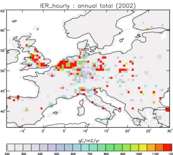
Fig. 1. Annual fossil fuel emissions from the “IER hourly”
inven-tory.
Figure 1 shows a map of the annual European “IER hourly” FFCO2emissions. The IER source has been interpolated to 0.5◦×0.5◦(large squares on the eastern part correspond to the “EDG annual” emission at 1◦×1◦). Large
emissions associated with industrial areas and big cities are well represented by this inventory. Note that the emissions over Germany show the highest level of detail, owing to the fact that much information was available to IER for this country (see Fig. 2).
2.1.5 Comparison of the different emissions inventories
Table 2 presents a comparison of annual FFCO2emissions for selected European countries and geographical Europe for the “EDG annual” and “IER hourly” inventories discussed above and the data reported by Marland et al. (2006). The latter is only used for further verification of country level FFCO2emissions. These estimates include emissions from all fossil sources except international shipping and air traffic at cruise altitude (landing and take off cycles are included) and cement production. The comparison indicates that the difference between the national totals is generally around 10 %. However, for some countries substantially larger dif-ferences are found, such as for the Netherlands, for which the difference between the estimates by EDGAR FT2000 and Marland et al. (2006) is 38 %. Similar differences are found for Norway (57 %), and Bulgaria (44 %). These differences are likely explained by inconsistencies, such as the exact def-inition of source classes, data gaps, etc. These inconsisten-cies are difficult to trace without support of inventory experts. In a recent study, Ciais et al. (2010) specifically analyzes the magnitude, trends, and uncertainties in FFCO2emission for EU-25, and show greater consistency between the
dif-Table 2. Comparison of annual fossil fuel emission estimates for
the year 2000.
Country EDGAR FT2000 IER Marland Max-Min PgC PgC PgC (%) Germany 0.262 0.234 0.224 15 France 0.119 0.111 0.099 18 Italy 0.130 0.126 0.122 6 Spain 0.089 0.084 0.082 8 England 0.162 0.148 0.154 9 Netherlands 0.057 0.047 0.039 38 Europe 1.989 1.752 – 13
ferent estimates (around 10 %) when differences in system boundaries (e.g. counting or not bunker fuels, non-energy products) are taken into account. However, when FFCO2 in-ventories are used by atmospheric modelers it is commonly assumed that they provide a systematic coverage of all fos-sil CO2 sources, and that the reported uncertainties repre-sent any deviations from that ideal situation. The accuracy of annual FFCO2emissions is therefore often assumed to be much better than 10 % (see for example R¨odenbeck et al., 2003; Baker et al., 2006; Bousquet et al., 2000). Our inven-tory comparison for Europe suggests that the differences can be substantially larger at the country scale (see also spatial differences between “IER hourly” and “EDG hourly” inven-tories, Fig. S1, Supplement). These differences give rise to what we refer to as “apparent uncertainty”, which is typi-cally substantially larger than the expected intrinsic uncer-tainty of the underlying data (like for example energy statis-tics). The differences are likely explained by numerous pos-sible inconsistencies arising from unaccounted sources,... In the end, however, the totals are most critical to atmospheric modelers and therefore the “apparent uncertainty” is critical when comparing models to atmospheric measurements, even though the numbers may be judged as unrealistically large by inventory experts.
Figure 2 shows a comparison of FFCO2temporal patterns in the emissions for selected countries. Sizeable emission variations are found, related, in particular, to the seasonal cycle (∼40 % peak-to-peak) and the diurnal cycle (∼80 % peak-to-peak). The seasonal variations provided by EMEP (as used in “EDG hourly”) are generally larger than those of IER. As expected, the seasonal emission variation in the Mediterranean countries is less than in more northern coun-tries owing to the mild Mediterranean climate in winter. This is illustrated by the difference between Italy and Germany in Fig. 2. This difference is more prominent for IER than for EMEP. Integrated over Europe the seasonal emission vari-ations of IER and EMEP are in relatively close agreement, although slightly smaller for IER. Note that the relative good agreement is at least partly explained by a substantial contri-bution of Eastern Europe, where EDGAR FT2000 replaces
Hourly fluxes (1 day) Daily fluxes (1 week) Weekly fluxes (1 year)
Eur
ope
Germany
Italy
Fig. 2. Temporal variation of the aggregated fluxes over different regions: Europe (top), Germany (middle) and Italy (bottom). First and
second columns represent the mean diurnal cycle and the mean weekly cycle, respectively, for “IER hourly” and “EDG hourly” in July and January; third column represents the seasonal variations (weekly means) for the four emissions inventories. Note that the y-range is different for Europe (much smaller).
missing IER estimates. In “EDG hourly” and “IER hourly” emissions the diurnal variation is larger than the weekly or seasonal variations all year long. The diurnal pattern of the EMEP emissions is less variable across different countries because the EMEP diurnal cycles do not include country specific information. For Germany, the IER emission vari-ations are about 50 % larger than those of EMEP in July, and only slightly larger in January. The morning and after-noon emission maxima are mainly determined by the peak in traffic rush hours. The relative size of these maxima shows slight differences between IER and EMEP. Figure 2 also shows the weekly emission variations in July and January. Smaller emissions (around 15 %) occur during the week-end than during the rest of the week in both “EDG hourly” and “IER hourly” emissions. EMEP and IER weekly varia-tions are in reasonable agreement, except for Germany where EMEP shows about 50 % less variation than IER. This sug-gests that the weekly emission variations in other countries might also be underestimated by EMEP, since the IER treat-ment of Germany is most realistic. All these differences are also illustrated for France and Spain in the Supplement (Fig. S2).
In summary, it can be concluded that the European fossil fuel emissions show significant temporal variation on vari-ous time scales (∼80 % on diurnal, ∼40 % on seasonal, and
∼15 % on weekly, peak-to-peak). Furthermore, these
vari-ations do not seem to be well quantified given the substan-tial differences between the estimates provided by EMEP and IER. The large differences between the “IER hourly” and the “EDG hourly” emission variations over Germany indicate the importance of using country specific information such as rush hour traffic, vacation periods, regional climate vari-ations,.... However, the important question is whether these variations give rise to significant variations in atmospheric FFCO2 sampled at surface stations. This question will be investigated in the following sections.
2.2 Transport model simulations
The fossil fuel emission inventories defined in Sect. 2.1 were prescribed as separate FFCO2 tracers to 7 transport models (see Table 3). Their horizontal resolutions vary between sev-eral square degrees (lat × lon) for the global models (LMDZ, TM3) to 0.5◦×0.5◦ for the regional models, which only
cover the European domain (DEHM, REMO, CHIMERE). TM5 reaches the highest resolution among the global mod-els, because it is zoomed over Europe at 1◦×1◦. CHIMERE slightly differs from the two other regional models, DEHM and REMO, as it only models the lower troposphere (up to 500 hPa) with a high vertical resolution (20 levels). COMET is a Lagrangian model in which the air mass trajectories are calculated from 3-hourly ECMWF meteorological fields at 1◦×1◦ horizontal resolution. Two vertical levels are
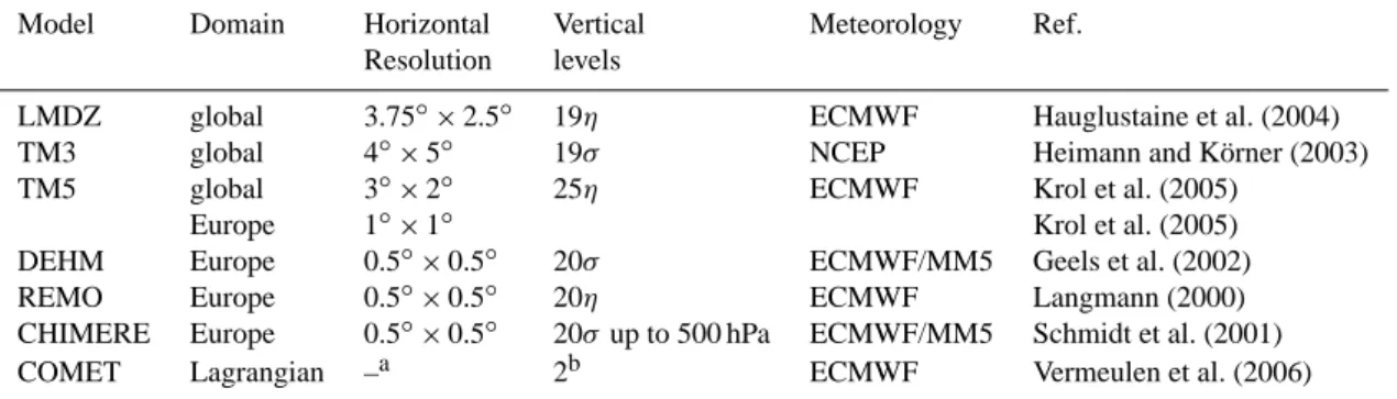
Table 3. Overview of participating atmospheric transport models.
Model Domain Horizontal Vertical Meteorology Ref. Resolution levels
LMDZ global 3.75◦×2.5◦ 19η ECMWF Hauglustaine et al. (2004) TM3 global 4◦×5◦ 19σ NCEP Heimann and K¨orner (2003) TM5 global 3◦×2◦ 25η ECMWF Krol et al. (2005)
Europe 1◦×1◦ Krol et al. (2005) DEHM Europe 0.5◦×0.5◦ 20σ ECMWF/MM5 Geels et al. (2002) REMO Europe 0.5◦×0.5◦ 20η ECMWF Langmann (2000) CHIMERE Europe 0.5◦×0.5◦ 20σ up to 500 hPa ECMWF/MM5 Schmidt et al. (2001) COMET Lagrangian –a 2b ECMWF Vermeulen et al. (2006)
aTrajectories calculation from meteorological fields at 1◦×1◦.
bLayer boundary at dynamically calculated PBL Height.
considered in COMET representing the planetary boundary layer and the free troposphere. Note, that COMET was pri-marily designed to simulate observational points that are in the mixed PBL. The vertical model resolution near the sur-face varies substantially between the models.The depth of the first layer ranges from 150 m in LMDZ/TM3 to nearly 30 m in REMO/CHIMERE. More detailed model descriptions can be found in Geels et al. (2007) and Law et al. (2008).
Model simulations were performed for 3 yr covering the period 2000–2002 (following the Transcom-3 experiment), using analyzed meteorology. The models were initialized at 0 ppm and the first two years are only used for spin-up. In the last year, concentrations are extracted at the same measure-ment sites used in the Transcom-3 model inter-comparison and at hourly temporal resolution for all models (Law et al., 2008). Hourly fields from the TM3 (or LMDZ) model were used as lateral boundary condition for the regional models, DEHM and REMO (or CHIMERE) and TM5 results were used as background information for COMET. Note finally, that nearly all models employ the ECMWF wind fields, ex-cept TM3 that uses NCEP winds.
2.3 Description of the inversions set-up
Inverse modeling calculations were performed to investigate the impact of the differences between fossil fuel inventories on the net exchange of carbon by the European terrestrial biosphere, inferred as a “residual”. Recall that in conven-tional inversions which neglect uncertainties of fossil fuel emissions the actual errors in the a priori fossil fuel inventory are projected on the a posteriori derived terrestrial biosphere fluxes. The aim of our inverse modeling calculations is to quantify this error. Although the accuracy of current inver-sions is known to be primarily limited by the sparseness of the atmospheric network, and by unknown biases in transport models (Gurney et al., 2002; Stephens et al., 2007), system-atic errors in fossil fuel space-time distribution might also turn out to be important.
Table 4. Set up of the two inversions.
LMDz inversion TM3 inversion
Flux resolution Monthly × Pixel based Weekly × Pixel based
Observations 70 sites; Monthly data 70 sites × Flask data
Prior fluxes Biosphere model (ORCHIDEE) No prior model
Prior errors Based on NPP + spatial correlations based on distance
We conducted a series of inversions with two transport models (TM3 and LMDZ) out of the seven described above. Currently both inversions solve for CO2surface fluxes at the spatial resolution of the model grid, given certain assump-tions on their prior error covariance matrix. The inverse set-ups follow from the study of Peylin et al. (2005) and ? for LMDZ and TM3, respectively. Both systems solve for the natural component of the terrestrial fluxes and for the ocean fluxes using atmospheric concentration measurements, atmo-spheric transport information, and prior information (includ-ing estimated a priori errors on the fluxes). The fossil fuel emissions are prescribed to the inversion, using either of the four inventories described in Sect. 2.1. The two systems are largely independent regarding their treatment of prior infor-mation, but adopt a similar selection of atmospheric stations (see Table 4 for details). The inversions are performed for the period 2000–2002, but we will only discuss the results for 2001, avoiding end effects (as caused both by the initial condition and the time lagged response of the fluxes at the stations).
For each model, we performed four inversions using the four different fossil fuel emission inventories. Note that in the case of LMDZ the diurnal cycle of the FFCO2 emis-sions is not used but only the day to day variations. In each case, only the land and ocean “residual” fluxes are optimized, while the fossil fuel component and its space-time distribution is assumed perfect and thus kept fixed. In a perfectly constrained inverse problem, i.e. with all fluxes
being independently constrained by atmospheric measure-ments, the differences between the inverted biosphere carbon fluxes would correspond to the differences in the input fossil fuel emissions. However, because of the under-constrained nature of current inversions (i.e., only few observations for a large number of unknown fluxes) the impact of fossil fuel dif-ferences might be significantly different, both spatially and temporally. These differences will also be spread over ad-jacent poorly constrained regions, including the oceans. We will thus compare the posterior fluxes (mainly over Europe) in order to investigate the sensitivity of the calculated bio-sphere flux to fossil fuel apparent uncertainties and the ne-glect of time variations in the prior fossil fuel emissions. The use of two different inverse approaches is important to deter-mine the sensitivities of the FFCO2induced emission biases to the choice of inversion procedure.
3 Results: forward modelling
3.1 FFCO2Concentration time series
CO2 concentration time series were simulated for all Eu-ropean measurements sites (see site location at http://www. carboeurope.org/). For the sake of brevity, the discussion is illustrated with the results for one station, the Hegyhatsal tall tower (115 m) in Hungary (referred to as “HUN”). Ad-ditional figures for HUN and for a second site Schauinsland (SCH, a mountain station in Germany that is usually incor-porated in inversions) can be found in the Supplement. We restricted ourself to these two sites as they can be considered representative of several European stations. To deal with the large number of factorial simulations, 7 transport models × 4 FFCO2emission inventories, we reduce the number of time series by displaying means across models and means across emissions, in order to compare the effect of emission pattern differences versus transport model differences on the simu-lated concentrations.
3.1.1 Seasonal cycle
Figure 3 (top) displays the daily mean FFCO2concentrations averaged across all models for each emission inventory at HUN. Like in most inversion set-ups, we selected daytime values (average over 10:00 h to 17:00 h LT), because existing transport models are known to have difficulties in simulating the stability of the nocturnal planetary boundary layer (PBL) (Geels et al., 2007). The simulated time series show large synoptic variations, up to 5 ppm, superimposed on a seasonal cycle of roughly the same size and a trend of few ppm yr−1 due to the accumulation of emitted FFCO2. These features are common to all stations (Fig. S3, Supplement), but the am-plitude of the synoptic events and the seasonal cycle varies depending on the location of the site to major industrialized regions. All tracers show a seasonal cycle, which in the case
of constant emissions reflects seasonal changes in the atmo-spheric transport, especially stronger mixing during summer than during winter over Europe. At HUN, the phase and am-plitude of the synoptic events are rather similar for all tracers, which indicates that the variation of atmospheric transport is the dominant factor causing day to day variations of FFCO2 at this site. Note that the observed amplitude of the synoptic CO2variations at HUN is roughly two times larger than the one obtained using FFCO2only.
Time series for the average across all emission invento-ries for each transport model (Fig. 3, middle), show simi-lar seasonal and synoptic patterns but with much less agree-ment for the amplitude and the timing of the synoptic events. On average the amplitude of the synoptic events is larger for the mesoscale models (REMO, DEHM, CHIMERE and COMET) and TM5 (zoomed model) than for the coarse global models (TM3 and LMDZ) and the differences be-tween models are largest in winter. Overall, the transport model spread dominates over the spread induced by the four different fossil fuel emissions. Similar results are found at all European stations (Supplement).
The effect of neglecting temporal variations in fossil fuel emission, is illustrated with the differences in simulated con-centration between “EDG hourly” and “EDG annual” emis-sions at HUN (Fig. 3 bottom). We observe a marked sea-sonality for all transport models with positive values in win-ter (up to 3 ppm) and slightly negative values in summer (up to −1 ppm). This difference combines (i) the seasonality of the “EDG hourly” source with (larger emissions in winter due to larger heating sources (∼50 %) compared to the con-stant “EDG annual” source; Sect. 2.1), and (ii) the season-ality of the atmospheric vertical mixing with the strongest mixing during summer time. Both effects act in the same di-rection and the amplitude of the resulting seasonal variation ranges from ±0.5 ppm at remote stations like Pallas in Fin-land up to ±5 ppm at stations close to industrial areas (i.e., the Cabauw tower in the Netherlands). Note that the covari-ance between seasonal variations in emissions and transport contributes about 1 ppm to the “seasonal rectifier effect” de-scribed for CO2by Keeling et al. (1989). The concentration differences between “IER hourly” and “EDG annual” emis-sions (not shown) show more complicated temporal patterns, indicating that spatial differences are as important as the ef-fect of neglecting the temporal variations in the emissions.
3.1.2 Diurnal cycle
Figure 4 (top) displays the hourly concentrations averaged across all transport models for each tracer at HUN for one week in July. A large diurnal cycle of up to 2 ppm is ob-served, with larger concentrations during nighttime than dur-ing daytime. For the constant emission fields (“T3 annual” and “EDG annual”), the simulated diurnal variations are fully explained by diurnal variations in the PBL height. For the time varying fluxes, increased fossil emissions during
HUN (115m) CO 2 concentration (ppm) CO 2 concentration (ppm) CO 2 concentration (ppm)
Fig. 3. Day-time mean simulated FFCO2 concentration at the Hungarian tall tower (HUN). Top: mean across all mean simulated FFCO2 concentration difference at HUN between “EDG hourly” and “EDG annual” fluxes transport models for each emission in-ventory; middle: mean across all emission inventory for each transport model; bottom: mean concentration difference between “EDG hourly” and “EDG annual”.
daytime oppose this effect and reduce the diurnal cycle in the simulated summer concentrations by up to 1–2 ppm depend-ing on the station. Similar results are ssupleen at all stations close to source regions. At remote stations or mountain sta-tions (SCH, Fig. S5, Supplement) the time series display al-most no diurnal cycle in summer. In winter, no clear diurnal cycle is observed at HUN and SCH (see Supplement): synop-tic events appear to be the dominant source of FFCO2short term variability, and both spatial and temporal differences between the emission inventories cause significant concen-tration differences (up to 4 ppm at HUN).
HUN (115m) CO 2 concentration (ppm) CO 2 concentration (ppm)
Fig. 4. Hourly simulated concentrations at HUN for 1 week in July: top: mean across all transport models for each emission inven-tory; bottom: mean across all emission inventories for each trans-port model.
Figure 4 (bottom) shows similar time series but now for the average across all tracers for each transport model. The scatter between the different transport models is much larger at all stations, with model to model differences up to 6 ppm, and complicated temporal patterns. For example, TM5 and partly COMET have a large diurnal cycle in summer with elevated FFCO2 concentrations at night compared to day-time (amplitude of nearly 5 ppm), unlike TM3 and LMDZ. In winter (see figures in Supplement), no clear coherent vari-ations can be discerned between the models at the daily time scale: synoptic events are clearly visible but their amplitudes strongly differ between models (from 2 ppm in TM3/LMDZ to 10 ppm in the other models).
3.2 Surface concentration fields
In order to further analyze the differences induced by trans-port models and emission inventories, we compare horizon-tal distributions of monthly mean mixing ratios at the surface for the full European domain sampled at 12:00 local time for January and July. We re-gridded the Eulerian model results for all tracers on a common resolution of 0.1 × 0.1 degree and for a layer between the surface and ∼ 150 m (to account for differences in vertical resolution). Figure 5 displays the
January July REMO LMDZ 10.0 11.0 12.0 13.0 14.0 15.0 16.0 17.0 18.0 19.0 20.0 22.0 25.0 30.0 35.0 40.0 45.0 ppm
Fig. 5. Comparison of fossil fuel CO2 fields as calculated by the highest (REMO) and the lowest resolution model (LMDZ) in-cluded in the inter-comparison, using “IER hourly” emission inven-tory. The numbers represent monthly averaged surface concentra-tions sampled at 12:00 local time. The surface layer is defined as 0–150 m above the ground.
concentration fields (averaged for the four emission invento-ries), for January and July, for REMO and LMDZ.
The high resolution model, REMO, resolves the spatial gradients caused by the FFCO2emissions much better than the coarser resolution model, LMDZ. Individual cities are re-solved (i.e., Madrid, Paris, London) and orography is clearly visible in REMO, while only the main emission regions are visible in LMDZ. In summer, FFCO2hot spots are less pro-nounced due to enhanced vertical mixing during daytime. As a direct consequence, the estimated fluxes from atmospheric inversion will be less sensitive to the spatial resolution of the FFCO2 emissions in summer. The two models agree on a larger trapping of FFCO2in the PBL in winter, but the East-ward shift of the maximum concentration compared to the emission map (Fig. 1) is more pronounced in the coarse res-olution model (LMDZ).
Two effects can explain the model differences. First, coarser models represent the FFCO2 emission at coarser resolution, thereby losing their ability to resolve individual cities. Secondly, higher resolution models better resolve the effects of mountains and land-sea transitions on winds and vertical mixing. To separate the two effects, the TM5 model was run with the emission resolution coarsened to the LMDZ resolution (see Supplement). The use of coarsened FFCO2emissions in TM5 already explains some of the dif-ferences between TM5 and LMDZ: for instance, the distinct FFCO2concentration maxima over the Netherlands and UK is lost when TM5 uses the coarser emissions. In conclusion, the higher spatial resolution of the emissions explains some, but not all of the differences observed between the various models. Schauinsland 1 2 3 4 5 6 7 8 9 10 11 12 2002 0 2 4 6 8 Δ CO 2 fossil fuel [ppm] Observations T3_annual EDG_annual EDG_hourly IER_hourly Schauinsland 1 2 3 4 5 6 7 8 9 10 11 12 2002 0 2 4 6 8 Δ CO 2 fossil fuel [ppm] Observations REMO DEHM TM3 TM5 LMDZ COMET CHIMERE
Fig. 6. Comparison of monthly-integrated fossil fuel CO2(relative
to Jungfraujoch) at Schauinsland based on14CO2observations with
simulations of all transport models using the “IER hourly” emission inventory (left panel) and with simulations of the regional model REMO using the four different emission inventories (right panel). An uncertainty estimate of observed monthly mean fossil fuel CO2
is included (grey shading).
3.3 Comparison with FFCO2based on14CO2
observations
Monitoring of fossil fuel CO2 is in principle possible with radiocarbon (14CO2) measurements in the PBL over the con-tinent (Levin et al., 2003). Spatial (or temporal) gradi-ents of 14CO2 reflect the excess fossil fuel CO2 that has been released in the air mass, given that fossil fuel CO2 is free of 14C. The current European network of stations with quasi-continuous time series of two-weekly or monthly-integrated14CO2 consists of seven stations, located in re-mote as well as in more polluted areas. Monthly-integrated FFCO2concentrations from all model simulations are com-pared with14CO2-based fossil fuel CO2observations for the year 2002. Figure 6 presents the results for the mountain sta-tion Schauinsland (SCH), which is often incorporated in in-versions, but additional results for the urban site Heidelberg (HEI) are provided in the Supplement (Fig. S8). Long-term
14CO
2measurements exist at both sites and regional fossil fuel CO2estimates are derived from these data in Levin et al. (2008). Analogous to the observations, the regional FFCO2 offset at each station was determined for the simulations us-ing Jungfraujoch high mountain station (Switzerland) as a background reference level.
At SCH the observed mean regional fossil fuel CO2 com-ponent is 1.5 ppm in 2002 and shows no significant seasonal cycle (Fig. 6). The simulation results of all transport mod-els using the “IER hourly” emissions show a large spread (Fig. 6, left panel) with annual mean values between 1.4 and 2.9 ppm and root mean square deviations from observations ranging from 0.5 to 1.6 ppm. The differences caused by the emission inventories, on the other hand, are significantly smaller (less than 0.5 ppm) than the deviations from the ob-servations (see left panel of Fig. 6 for REMO model).
A quantitative evaluation of the transport model perfor-mances using14C-based fossil fuel CO2observations is dif-ficult because of compensating effects between transport
model deficiencies, spatial resolution, and emission errors. For instance, LMDZ simulations show relatively good agree-ment with the14C data despite the coarse horizontal and ver-tical resolution of the model. On the other hand, high resolu-tion models, which are more sensitive to the exact locaresolu-tion of emission sources in the vicinity of a station, and which pre-sumably better resolve transport characteristics, tend to de-viate more. This is even more obvious at the Heidelberg ur-ban site, where the the REMO simulations are almost twice the14C-based fossil fuel CO2 observation. The spread be-tween all transport model simulations at Heidelberg is also larger than the deviations from the observations. There is also a clear seasonal cycle at this station both in the obser-vations and the model simulations. While the coarse reso-lution models are generally not very sensitive to differences between FFCO2emission inventories, even at a polluted site, the high-resolution models show a clear improvement of the seasonal cycle at HEI if the inventory includes temporal vari-ability. This result opens for further applications of the14C approach.
4 Impact on inversion of ecosystem fluxes
In this section, we investigate the significance of the differ-ences between the fossil fuel emission inventories by quan-tifying their impact on the optimized biosphere fluxes. We compare the inverted ecosystem fluxes (Fbio) from different inversions for 2001, using the four different fossil fuel emis-sion inventories. We use the “EDG annual” constant FFCO2 inversion as the “reference” case since this represents the commonly applied assumption in global inverse modelling. We then investigate the differences obtained when using the other inventories. We first discuss the annual mean of Fbio over Europe and then spatial differences (Fig. 7).
4.1 Monthly Fbio fluxes
For all inversions, the monthly European Fbio flux shows a large seasonal cycle (as expected) with a maximum carbon uptake in June (see Supplement). The amplitude of the sea-sonal cycle is roughly 1 GtC month−1integrated over Europe (12.106km2). Differences between fossil fuel inventories (each case versus the reference) induce Fbio differences of less than 0.04 GtC month−1, which is very small compared to the seasonal cycle and much lower than the estimated Bayesian uncertainty returned by the inversions (in the or-der of 0.1 GtC month−1). Logically, accounting for temporal variations on the fossil fuel emissions (“EDG hourly” ver-sus “EDG annual”) decreases the estimated biosphere flux in winter and increases it during summer, as a compensa-tion for the seasonality imposed on the fossil fuel emissions (“EDG hourly”). If we consider smaller regions, like the “western part” of Europe, the impact of the temporal vari-ations of fossil fuel emissions on the derived monthly Fbio
fluxes becomes slightly larger when compared to the ampli-tude of the seasonal cycle but remains below 5 %. These results are consistent across the two inverse set ups (LMDZ and TM3).
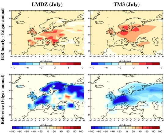
Figure 7 now illustrates for July the spatial distribution of the impact of fossil fuel emission inventories on Fbio. We compare the results using “EDG annual” (reference case, bottom panel) to the differences between using “IER hourly” and “EDG annual” (top panel). For this particular month, the differences obtained with the “LMDZ” or “TM3” inver-sions appear to be on the order of 2 to 6 gC m−2month−1 across a large part of Europe (with maximum values close to 10 gC m−2month−1) while the reference Fbio shows car-bon uptake between 20 and 100 gC m−2month−1in the same area. On a country scale, a change of fossil fuel emis-sion inventory could thus significantly affect the Fbio flux: for each country the averaged impact can reach in our case 20 % in July. The same calculation obtained between using “EDG hourly” and “EDG annual” (not shown) show smaller differences in LMDZ but similar differences in TM3. The TM3 result indicates that temporal variations in fossil fuel emissions can induce regionally significant differences in the estimated monthly Fbio. The smaller difference with LMDZ comes from the fact that this inversion system did not ac-count for the diurnal variations in FFCO2 emissions (see Sect. 2.3). These Fbio differences can directly be compared to the differences between the emission maps themselves. The differences between “IER hourly” and “EDG annual” fossil fuel sources for July (Fig. S1, Supplement) can reach
±100 gC m−2month−1 over industrial areas (i.e., Western Germany). This result confirms that the inversions tend to smooth these large FFCO2 emission differences and dis-tribute them spatially over adjacent regions. These results hold for all months and reflect the under-constrained nature of current inversions.
4.2 Annual Fbio fluxes
Integrated over the year, the differences in estimated Fbio be-come much more significant than at the monthly time scale (Table 5). The effect of accounting for temporal variations in fossil fuel emissions (“EDG hourly” versus “EDG annual”) on the Fbio estimates is limited to less than 5 % (integrated over Europe or its “Western part”), but the effect of switching emission patterns and magnitudes lead to much larger dif-ferences. For instance, using the “IER hourly” emission in-ventory changes the mean value of Fbio by ∼0.15 GtC yr−1 for the whole Europe and by ∼0.05 GtC yr−1for the West-ern part. These numbers are slightly smaller than the an-nual total European differences in fossil fuel emissions them-selves (0.23 GtC yr−1 for Europe, Table 2) because part of the fossil fuel difference is compensated by Fbio (and Fo-cean) flux adjustments outside Europe (see Fig. 8). The use of the “T3 annual” emissions induces smaller changes (less than 20 % integrated over Europe). Overall, the largest fossil
Table 5. Annual inverse estimate of the net biological fluxes (Fbio, in GtC yr−1) based on the Edgar annual fossil fuel CO2emissions
inventory (including the estimated posterior uncertainty for total Europe ±1σ ) and differences in Fbio resulting from the use of the other three inventories, for the LMDZ and TM3 inversions. (*): not estimated.
Flux using Flux differences
Edgar ann Edgar hr IER hr Transcom – Edgar ann – Edgar ann – Edgar ann LMDZ Tot Europe −0.35 (± 0.33) −0.01 0.14 0.06 LMDZ West Europe −0.03 (*) −0.00 0.05 0.02 TM3 Tot Europe −0.57 (± 0.25) 0.01 0.15 0.11 TM3 West Europe −0.41 (*) 0.00 0.03 0.01
LMDZ (July)
TM3 (July)
IER hourly -Edgar annual Refer ence (Edgar annual)Fig. 7. July biosphere fluxes estimated with the LMDZ and TM3 inversions (see text for methodology) for a case using “EDG annual” fossil
fuel emissions (lower panels) and the difference between using “IER hourly” and “EDG annual” emissions (upper panels).
difference corresponds to 26 % difference and 40 % differ-ence of the annual Fbio for Europe estimated for that par-ticular year (2001) in the two inversions completed in this study, respectively. The posterior Bayesian uncertainties on Fbio fluxes estimated by the two inversion systems (only cal-culated for total Europe, Table 5) indicate that (i) the two different estimates are statistically compatible (i.e. within the 0.3 GtC yr−1 estimated uncertainty) and (ii) the differ-ences induced by using different fossil fuel inventories are also within 1 sigma of the posterior error. Note that the two inversion-derived annual Fbio fluxes for Europe are of the same magnitudes than the mean fluxes estimated by Janssens et al. (2003).
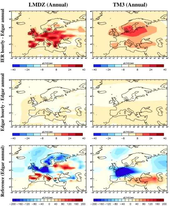
If we now consider the spatial distribution of the an-nual Fbio fluxes (Fig. 8), larger differences than for July are found. First, the mean flux with the “EDG annual” FFCO2 emission (Fig. 8-bottom) presents much larger re-gional variations in the LMDZ inversion (than in TM3) that are related to the strong influence of the prior flux distribu-tion in this system (taken from a biogeochemical model, see Sect. 2.3). A detailed analysis of the differences between the two systems is beyond the scope of this paper. The Fbio differences between using “IER hourly” and “EDG annual” FFCO2emissions are significant, and up to 50 gC m−2yr−1 over specific regions like the Netherlands while the original flux FFCO2flux difference is around 250 gC m−2yr−1(i.e.,
LMDZ (Annual)
TM3 (Annual)
IER hourly -Edgar annual Edgar hourly -Edgar annual Refer ence (Edgar annual)Fig. 8. Annual biosphere fluxes estimated with the LMDZ and TM3 inversions (see text for methodology) for a case using “EDG annual”
fossil fuel emissions (lower panels) and the differences between using “IER hourly” and “EDG annual” emissions (upper panels) and be-tween using “EDG hourly” and “EDG annual” emissions (middle panels).
0.01 GtC yr−1, Table 2). However, the difference between using “EDG hourly” and “EDG annual” is proportionally much smaller (unlike for July fluxes), which indicates that the temporal variations in FFCO2emissions have a negligible impact on the annual Fbio flux, at least given the resolution of transport models used in the two inversions.
Overall these sensitivity tests highlight the increasing im-pact of uncertainties (mainly biases) in fossil fuel emission inventories on the estimated biosphere fluxes from the con-tinental to the regional scale. However, further investigation need to be carried out with inverse systems at higher spatial resolution (at least 0.5 degree) in order to use all the
informa-tion contained in the new high resoluinforma-tion FFCO2 emission inventories (i.e., “IER hourly”). These systems will be more adapted to investigate separately the effect of diurnal, day to day, and seasonal variations in fossil fuel emissions on the estimated Fbio fluxes.
5 Discussion: transport versus FFCO2emission errors
We have shown the impact of differences in current fos-sil fuel emission inventories on modeled FFCO2 concentra-tions at European staconcentra-tions and further assessed the impact on
0.0 0.2 0.4 0.6 0.8 1.0 1.2 1.6 2.0 2.4 2.8 3.2 4.0 6.0 8.0 ppm July Jan. Tracer Std. Model Std.
Fig. 9. Standard deviation of monthly averaged fossil fuel CO2
concentrations. Standard deviations are calculated either for the mean FFCO2 emission inventories across the transport models
(left), or for the mean transport model across the FFCO2emission inventories (right). Monthly mean averaged surface concentrations are calculated as in Fig. 5.
two state of the art atmospheric inversions. In Sect. 3.1 it was demonstrated that the atmospheric transport model dif-ferences have a substantially larger impact on FFCO2 con-centrations than the differences between emission invento-ries. To investigate this issue further, we calculated the mean concentration field and the corresponding standard deviation (std-dev) when varying either the emissions or the atmo-spheric transport. The computation involves two steps. In the first one, we compute the std-dev of the concentrations obtained with a given transport-model (FFCO2-tracer) and all FFCO2-tracers (transport-models). In the second one, we average the different standard deviations to obtain a mean value. We verified that the ratios between the two std-devs (transport vs. emissions, as discussed below) are robust and not sensitive to the small sample sizes (7 transport models and 4 emissions), using the spread of the concentration fields as a metric. The results, analyzed for January and July, at 12:00 local time (Fig. 9) clearly confirms the findings from Sect. 3.1. Standard deviation from the transport models (
σtrsp, left panels) are substantially larger than std-dev from the emissions (σemis, right panels), both in January and in July.
Moreover, the std-dev are larger in winter compared to the summer, due to enhanced wintertime trapping of the emis-sions. Away from large emission sources, σemisand σtrspare rather small, although the transport models show consider-able disagreement over the Atlantic Ocean in summer (σtrsp
∼1 ppm). This is linked to large differences in PBL mixing and wind fields between the models in summer. Interestingly, the largest variability among the transport models is not al-ways found just over the emission areas, but for instance over the Alps, where σtrsp reaches up to 8 ppm in winter. Obvi-ously, high resolution models resolve the emission, orogra-phy, and the associated transport patterns better than coarse
Table 6. Annual averaged standard deviation of Hourly/monthly
averaged fossil fuel CO2concentrations (ppm) at a few stations for
the whole year. Standard deviations were calculated either for the mean CO2emission tracer across the transport models, or for the
mean transport model across the CO2emission tracers.
station Transport Tracer Hourly/Monthly Hourly/Monthly BSC 0.99/0.58 0.50/0.46 CMN 1.07/0.90 0.23/0.22 HUN115 1.46/0.94 0.59/0.51 MHD 0.75/0.52 0.24/0.22 SCH 1.13/0.73 0.35/0.29 SAC 2.34/1.69 1.16/1.07
resolution models. Concerning σemis, the largest variability appears in areas with large emissions (see Fig. 1). It is indeed at these locations that the emission inventories differ in their spatial and temporal patterns. Depending on the location, the ratio between σtrsp and σemisvaries between 2 and 8 (larger model differences) with maximum ratios in January.
If we now consider the station locations where current CO2 measurements take place, Table 6 compares σtrsp and
σemis computed for the whole year using hourly or monthly mean values. For the sites that are currently used in most atmospheric inversion (HUN, Mace Head (MHD), Schauins-land (SCH), Monte Cimone (CMN)) the hourly FFCO2 spread caused by the transport model differences (between 1 and 2 ppm) appears to be ∼3 times larger than the spread caused by the emission inventories. Using monthly mean concentrations reduce the difference to a factor 2.5, with σtrsp and σemis around 0.7 ppm and 0.3 ppm, respectively. These numbers indicate that although transport model uncertainties dominate over Europe, differences in annual fossil fuel es-timates or neglecting their temporal variations also play a critical role. If we now consider stations that are closer to anthropogenic emission areas, like Black Sea Coast (BSC) and Saclay (SAC) near Paris, the ratio between transport model spread and emission spread becomes on the order of two or even less. The assimilation of observed concentra-tions at these sites would increase the sensitivity of inverse modeling-derived biosphere fluxes to fossil fuel uncertain-ties.
6 Conclusions
We analyzed the importance of differences between fossil-fuel CO2 emission inventories and the importance of sub-annual variations in these emissions for tracer transport mod-elling and regional scale inverse modmod-elling of the Euro-pean C-cycle, by testing four alternative fossil fuel inven-tories. Although fossil-fuel emissions are often considered as a “well known” term in the terrestrial carbon balance,
annual differences between emission inventories are typi-cally ∼10 % at the country level reaching up to 40 % for some European countries. These differences increase with decreasing length scale, and correspond to systematic errors due to inconsistent accounting systems (i.e. see for instance Ciais et al. (2010)). Seasonal and diurnal variations in fossil fuel emissions, which are commonly neglected, reach ampli-tudes close to 40 % and 80 %, respectively.
The significance of these emission differences for inverse modelling depends on how they relate to other sources of un-certainty. We have investigated their relative importance in comparison with transport model uncertainties, which also addresses the question of whether fossil fuel CO2could be used as a diagnostic tracer for testing atmospheric transport or if atmospheric CO2inversions can be used to evaluate fos-sil fuel CO2 emissions. The impact of the fossil-fuel emis-sion uncertainties on modeled FFCO2concentrations at the European stations is on the order of 0.4 ppm (std-dev calcu-lated with the same model but different emissions) while the impact of using several transport models with the same emis-sion is 2–3 times larger, depending on the location and period of the year. We additionally quantified the impact of fossil fuel uncertainties on two state of the art global inversions. Monthly changes in estimated biosphere fluxes at the Euro-pean scale are small and less than 4 % but annual changes become critical, as expected from the differences in annual emission totals. Differences up to 0.15 GtC yr−1are of sim-ilar magnitude as the total European carbon sink estimated by Janssens et al. (2003). However these impacts and espe-cially the impacts from incorrect specification of fine tem-poral and spatial emission distributions could potentially be much larger with meso-scale inversion systems.
These results indicate that uncertainties in fossil fuel emis-sion inventories cannot be ignored in applications of inverse modelling of the European C-cycle, and that in order to ad-vance our understanding of the net carbon exchange of the European terrestrial biosphere, the consistency of the Euro-pean fossil fuel inventories needs substantial improvement. Not only the national and annual scales but also finer spa-tial and temporal scales need to be improved to aid regional modelling studies. Sub-annual FFCO2 emission variations lead to significant changes in the seasonal and diurnal con-centration variations at the European stations of up to few ppm (∼2 ppm at HUN).
We have used emission inventories for one particular year (2000) but there is a need for similar high-resolution inven-tories for subsequent years to account for changing emis-sions associated to the economic development and for CO2 emissions that are dependent on the meteorological condi-tions such as domestic heating. Within the North American Carbon Project (NACP), the “VULCAN” project (Gurney et al., 2009) is going in this direction with a recent release of a new emission inventory for North America at hourly time scale on a 10 km grid. Several efforts are also ongoing in Europe within EDGAR and IER groups but also within
national agencies. These efforts need to be continued, har-monized, and validated at several levels of the data process-ing chain. For example, the IER emission inventory used in this study is much more precise for Germany than for other countries, which can lead to systematic FFCO2 concentra-tion differences between staconcentra-tions and induce critical biases in the inversion results. We also anticipate that country spe-cific information for rush hour traffic, vacation periods, or the type of consumed energy (fossil, renewable, nuclear) will di-rectly impact the temporal emission distributions. The use of higher resolution transport model (such as REMO) will pro-duce larger temporal and spatial concentration gradients (see Sect. 3.2), which will in turn directly impact the retrieved biosphere fluxes.
Finally, monitoring of fossil fuel CO2is in principle possi-ble with radiocarbon (14CO2) measurements in the PBL over the continent (Levin et al., 2003). Currently14CO2is mea-sured quasi-continuously only at very few stations in Europe and mostly integrated over time periods of one or several weeks. From first comparisons of the model simulations with monthly14C-based fossil fuel CO2 observations it was not yet possible to discriminate between the four FFCO2 emis-sion inventories. Moreover, the large differences between simulated and observed FFCO2 call for a further system-atic evaluation of the transport characteristics in the mod-els. High-resolution time series of FFCO2, which are based on a combination of hourly CO measurements with weekly-integrated14CO2measurements (Levin and Karstens, 2007), will become available at several stations and will allow a more detailed analysis of diurnal to synoptic scale differ-ences. However, current observation systems do not allow yet to accurately attribute observed CO2concentration vari-ations on daily/weekly timescales. Overall, improvements of the transport models are clearly needed before an inde-pendent verification of emission inventories through compar-isons of simulated and observed fossil fuel CO2 might be-come feasible.
Supplementary material related to this article is available online at:
http://www.atmos-chem-phys.net/11/6607/2011/ acp-11-6607-2011-supplement.pdf.
Acknowledgements. We thank the research group of IER for the
construction of a detailed European fossil fuel emission inventory, within the CarboEurope Integrated Program (CE-IP). CE-IP also partly funded this work and resources for the different simulations. We also thank Ingeborg Levin for providing the monthly-integrated fossil fuel CO2 based on 14CO2 observations available in the CarboEurope database.
The publication of this article is financed by CNRS-INSU.
References
Baker, D. F., Law, R. M., Gurney, K. R., Rayner, P., Peylin, P., Denning, A. S., Bousquet, P., Bruhwiler, L., Chen, Y.-H., Ciais, P., Fung, I. Y., Heimann, M., John, J., Maki, T., Maksyu-tov, S., Masarie, K., Prather, M., Pak, B., Taguchi, S., and Zhu, Z.: TransCom 3 inversion intercomparison: Impact of transport model errors on the interannual variability of regional CO2fluxes, 1988–2003, Global Biogeochem. Cy., 20, GB1002, doi:10.1029/2004GB002439, 2006.
Bousquet, P., Peylin, P., Ciais, P., Quere, C. L., Friedlingstein, P., and Tans, P. P.: Regional changes in carbon dioxide fluxes of land and oceans since 1980, Science, 290, 1342–1346, 2000. Brenkert, A. L.: Carbon Dioxide Emission Estimates from
Fossil-Fuel Burning, Hydraulic Cement Production, and Gas Flaring for 1995 on a One Degree Grid Cell Basis, Document file for database NDP-058a 2-1998, Oak Ridge National Laboratory, Oak Ridge, Tennessee, 1998.
Canadell, J. G., Le Quere, C., Raupach, M. R., Field, C. B., Buiten-huis, E. T., Ciais, P., Conway, T. J., Gillett, N. P., Houghton, R. A., and Marland, G.: Contributions to accelerating atmo-spheric CO2growth from economic activity, carbon intensity,
and efficiency of natural sinks, P. Natl. Acad. Sci. USA, 104, 18866–18870, doi:10.1073/pnas.0702737104, 2007.
Ciais, P., Paris, J., Marland, G., Peylin, P., Piao, S., Levin, I., Pregger, T., Scholz, Y., Friedrich, R., Houwelling, S., and Schulze, D.: The European carbon balance revisited. Part 1: fossil fuel emissions, Glob. Change Biol., 16, 1395–1408, doi:10.1111/j.1365-2486.2009.02098.x, 2010.
Denning, A. S., Fung, I., and Randall, D.: Latitudinal gradient of atmospheric CO2due to seasonal exchange with land biota,
Na-ture, 376, 240–243, 1995.
Geels, C., Christensen, J. H., Frohn, L. M., and Brandt, J.: Simulat-ing spatiotemporal variations of atmospheric CO2using a nested hemispheric model, Phys. Chem. Earth, 27, 1495–1506, 2002. Geels, C., Gloor, M., Ciais, P., Bousquet, P., Peylin, P., Vermeulen,
A. T., Dargaville, R., Aalto, T., Brandt, J., Christensen, J. H., Frohn, L. M., Haszpra, L., Karstens, U., R¨odenbeck, C., Ra-monet, M., Carboni, G., and Santaguida, R.: Comparing at-mospheric transport models for future regional inversions over Europe – Part 1: mapping the atmospheric CO2 signals, At-mos. Chem. Phys., 7, 3461–3479, doi:10.5194/acp-7-3461-2007, 2007.
Gurney, K. R., Law, R. M., Denning, A. S., Rayner, P., Baker, D., Bousquet, P., Bruhwiler, L., Chen, Y., Ciais, P., Fan, S., Fung, I. Y., Gloor, M., Heimann, M., Higuchi, K., John, J., Maki, T., Maksyutov, S., Masarie, K., Peylin, P., Prather, M., Pak, B. C., Randerson, J., Sarmiento, J., Taguchi, S., Takahashi, T., and Yuen, C.: Towards robust regional estimates of CO2sources and
sinks using atmospheric transport models, Nature, 415, 626–630, 2002.
Gurney, K., Chen, Y., Maki, T., Kawa, S., Andrews, A., and Zhu, Z.: Sensitivity of atmospheric CO2 inversions to seasonal and
interannual variations in fossil fuel emissions, J. Geophys. Res.-Atmos., 110(D10), 10308–10321, doi:10.1029/2004JD005373, 2005.
Gurney, K., Mendoza, Z., Zhou, Y., Fischer, M., de la Rue du Can, S., Geethakumar, S., and Miller, C.: High resolution fossil fuel combustion CO2 emissions fluxes for the United States, Environ. Sci. Technol., 43, 5535–5541, 2009.
Hauglustaine, D. A., Hourdin, F., Jourdain, L., Filiberti, M.-A., Walters, S., Lamarque, J.-F., and Holland, E. A.: Interac-tive chemistry in the Laboratoire de M´et´eorologie Dynamique general circulation model: Description and background tropo-spheric chemistry evaluation, J. Geophys. Res., 109, D04314, doi:10.1029/2003JD003957, 2004.
Heimann, M. and K¨orner, S.: The global atmospheric tracer model TM3, Model description and user’s manual Release 3.8a, Max Planck Institute of Biogeochemistry, 2003.
Janssens, I., Freibauer, A., Ciais, P., Smith, P., Nabuurs, G., Folberth, G., Schlamadinger, B., Hutjes, R., Ceule-mans, R., Schulze, E., Valentini, R., and Dolman, A.: Europe’s terrestrial biosphere absorbs 7 to 12 % of Euro-pean anthropogenic CO2emissions, Science, 300, 1538–1542,
doi:10.1126/science.1083592, 2003.
Keeling, C. D., Bacastow, R. B., Carter, A. F., Piper, S. C., Whorf, T. P., Heimann, M., Mook, W. G., and Roeloffzen, H. A.: A three-dimensional model of atmospheric CO2transport based on
observed winds: 1. Analysis of observational data, in: Aspects of climate variability in the Pacific and the Western Americas, Geophysical monograph 55, edited by: Peterson, D. H., 165– 236, AGU, 1989.
Krol, M., Houweling, S., Bregman, B., van den Broek, M., Segers, A., van Velthoven, P., Peters, W., Dentener, F., and Bergamaschi, P.: The two-way nested global chemistry-transport zoom model TM5: algorithm and applications, Atmos. Chem. Phys., 5, 417– 432, doi:10.5194/acp-5-417-2005, 2005.
Langmann, B.: Numerical modelling of regional scale transport and photochemistry directly together with meteorological processes, Atmos. Environ., 34, 3585–3598, 2000.
Law, R. M., Peters, W., R¨odenbeck, C., et al.: TRANSCOM model simulations of hourly CO2: experimental overview and
diur-nal results for 2002, Global Biogeochem. Cy., 22, GB3009, doi:10.1029/2007GB003050, 2008.
Levin, I. and Karstens, U.: Inferring high-resolution fossil fuel CO2 records at continental sites from combined (CO2)-C-14 and
CO observations, Tellus B, 59, 245–250, doi:10.1111/j.1600-0889.2006.00244.x, 2007.
Levin, I., Kromer, B., Schmidt, M., and Sartorius, H.: A novel ap-proach for independent budgeting of fossil fuel CO2over Eu-rope by14CO2observations, Geophys. Res. Lett., 30(23), 2194,
doi:10.1029/2003GL018477, 2003.
Levin, I., Hammer, S., Kromer, B., and Meinhardt, F.: Ra-diocarbon observations in atmospheric CO2: Determining
fossil fuel CO2 over Europe using Jungfraujoch
observa-tions as background, Sci. Total Environ., 391, 211–216, doi:10.1016/j.scitotenv.2007.10.019, 2008.
National Fossil Fuel CO2Emissions. In Trends: A Compendium of Data on Global Change, US department of energy, Carbon Dioxide Information Analysis Center, Oak Ridge National Lab-oratory, Oak Ridge, Tenn., USA, 2006.
Peylin, P., Rayner, P. J., Bousquet, P., Carouge, C., Hourdin, F., Heinrich, P., Ciais, P., and AEROCARB contributors: Daily CO2 flux estimates over Europe from continuous atmospheric
measurements: 1, inverse methodology, Atmos. Chem. Phys., 5, 3173–3186, doi:10.5194/acp-5-3173-2005, 2005.
Pregger, T., Scholz, Y., and Friedrich, R.: Documentation of the anthropogenic GHG emission data for Europe provided in the Frame of CarboEurope GHG and CarboEurope IP, Project re-port, available at: http://www.carboeurope.org/ section: prod-uct/article/report, 2007.
R¨odenbeck, C., Houweling, S., Gloor, M., and Heimann, M.: CO2
flux history 1982–2001 inferred from atmospheric data using a global inversion of atmospheric transport, Atmos. Chem. Phys., 3, 1919–1964, doi:10.5194/acp-3-1919-2003, 2003.
Schmidt, H., Derognat, C., Vautard, R., and Beekmann, M.: A com-parison of simulated and observed ozone mixing ratios for the summer of 1998 in Western Europe, Atmos. Environ., 36, 6277– 6297, 2001.
Stephens, B. B., Gurney, K. R., Tans, P. P., Sweeney, C., Pe-ters, W., Bruhwiler, L., Ciais, P., Ramonet, M., Bousquet, P., Nakazawa, T., Aoki, S., Machida, T., Inoue, G., Vinnichenko, N., Lloyd, J., Jordan, A., Heimann, M., Shibistova, O., Langen-felds, R. L., Steele, L. P., Francey, R. J., and Denning, A. S.: Weak northern and strong tropical land carbon uptake from ver-tical profiles of atmospheric CO2, Science, 316, 1732–1735,
doi:10.1126/science.1137004, 2007.
van Aardenne, J. A., Dentener, F. J., Olivier, J. G. J., Peters, J. A. H. W., and Ganzeveld, L. N.: The EDGAR 3.2 Fast track 2000 dataset (32FT2000), Tech. rep., Joint Research Centre (JRC), Ispra, Italy, available at: http://www.mnp.nl/edgar/model/ v32ft2000edgar, 2005.
Vermeulen, A. T., Pieterse, G., Hensen, A., van den Bulk, W. C. M., and Erisman, J. W.: COMET: a Lagrangian transport model for greenhouse gas emission estimation – forward model technique and performance for methane, Atmos. Chem. Phys. Discuss., 6, 8727–8779, doi:10.5194/acpd-6-8727-2006, 2006.
Vestreng, V., Breivik, K., Adams, M., Wagener, A., Goodwin, J., Rozovskkaya, O., and Pacyna, J. M.: Inventory Review 2005, Emission Data reported to LRTAP Convention and NEC Direc-tive, Initial review of HMs and POPs, MSC-W 1/2005 ISSN 0804-2446, EMEP, 2005.