HAL Id: insu-00787159
https://hal-insu.archives-ouvertes.fr/insu-00787159
Submitted on 6 Jan 2016
HAL is a multi-disciplinary open access
archive for the deposit and dissemination of
sci-entific research documents, whether they are
pub-lished or not. The documents may come from
teaching and research institutions in France or
abroad, or from public or private research centers.
L’archive ouverte pluridisciplinaire HAL, est
destinée au dépôt et à la diffusion de documents
scientifiques de niveau recherche, publiés ou non,
émanant des établissements d’enseignement et de
recherche français ou étrangers, des laboratoires
publics ou privés.
Calibration and evaluation of a semi-distributed
watershed model of Sub-Saharan Africa using GRACE
data
H. Xie, Laurent Longuevergne, C. Ringler, B. R. Scanlon
To cite this version:
H. Xie, Laurent Longuevergne, C. Ringler, B. R. Scanlon. Calibration and evaluation of a
semi-distributed watershed model of Sub-Saharan Africa using GRACE data. Hydrology and Earth System
Sciences, European Geosciences Union, 2012, 16 (9), pp.3083-3099. �insu-00787159�
www.hydrol-earth-syst-sci.net/16/3083/2012/ doi:10.5194/hess-16-3083-2012
© Author(s) 2012. CC Attribution 3.0 License.
Hydrology and
Earth System
Sciences
Calibration and evaluation of a semi-distributed watershed
model of Sub-Saharan Africa using GRACE data
H. Xie1, L. Longuevergne2, C. Ringler1, and B. R. Scanlon3
1International Food Policy Research Institute, 2033 K Street NW, Washington D.C. 20006, USA
2CNRS – UMR 6118, G´eosciences Rennes Universit´e Rennes 1, 35042 Rennes, France
3Bureau of Economic Geology, Jackson School of Geosciences, University of Texas, Austin, TX 78713-8926, USA
Correspondence to: H. Xie (h.xie@cgiar.org)
Received: 29 December 2011 – Published in Hydrol. Earth Syst. Sci. Discuss.: 17 February 2012 Revised: 25 June 2012 – Accepted: 1 July 2012 – Published: 3 September 2012
Abstract. Irrigation development is rapidly expanding in mostly rainfed Sub-Saharan Africa. This expansion under-scores the need for a more comprehensive understanding of water resources beyond surface water. Gravity Recovery and Climate Experiment (GRACE) satellites provide valu-able information on spatio-temporal variability in water stor-age. The objective of this study was to calibrate and evalu-ate a semi-distributed regional-scale hydrologic model based on the Soil and Water Assessment Tool (SWAT) code for basins in Sub-Saharan Africa using seven-year (July 2002– April 2009) 10-day GRACE data and multi-site river dis-charge data. The analysis was conducted in a multi-criteria framework. In spite of the uncertainty arising from the trade-off in optimising model parameters with respect to two non-commensurable criteria defined for two fluxes, SWAT was found to perform well in simulating total water storage vari-ability in most areas of Sub-Saharan Africa, which have semi-arid and sub-humid climates, and that among various water storages represented in SWAT, water storage varia-tions in soil, vadose zone and groundwater are dominant. The study also showed that the simulated total water storage vari-ations tend to have less agreement with GRACE data in arid and equatorial humid regions, and model-based partitioning of total water storage variations into different water storage compartments may be highly uncertain. Thus, future work will be needed for model enhancement in these areas with in-ferior model fit and for uncertainty reduction in component-wise estimation of water storage variations.
1 Introduction
Sub-Saharan Africa (SSA) is used as a collective term that refers to African nations which lie (or partially lie) south of the Sahara. The region makes up about 80 % of the African and 10 % of the global population. Agriculture forms the backbone of the SSA economy; however, SSA countries largely missed the green revolution. The agricultural produc-tivity in SSA countries remains low relative to other parts of the world and the region is still beset with food insecu-rity. The number of estimated undernourished people in SSA in 2010 reached 239 million (FAO, 2010). SSA is also the only region where childhood malnutrition is projected to in-crease as a result of rapid population growth, climate change and continued low productivity in agriculture (Rosegrant et al., 2009). Annual population growth in SSA is 2.2 %, much higher than global average of 1.1 % (World Bank, 2009). In addition, SSA is regarded as the region with a particularly low capacity to adapt to climate change (IPCC, 2007).
Sustainable intensification of agriculture, with a focus on irrigation development, is considered a key pillar for increas-ing agricultural productivity in SSA (Rosegrant et al., 2002; Molden, 2007; Rockstr¨om et al., 2007). SSA straddles the Equator and is dominated by tropical and sub-tropical cli-mate. Rainfall in SSA is highly variable both spatially and temporally and constitutes a more critical factor than tem-perature for agriculture. Limited water availability, particu-larly during droughts, is a key reason for crop failure, espe-cially considering the fact that SSA agriculture is predomi-nantly rainfed with only 3 % of the cultivated area irrigated (Siebert, 2010; FAO, 2011). Both international development
3084 H. Xie et al.: Semi-distributed watershed model of Sub-Saharan Africa using GRACE data banks and African governments have pledged to significantly
increase irrigation development to address low agricultural productivity, rural poverty and food security challenges in the region.
Significant expansion of irrigated agriculture in SSA, how-ever, will require a more comprehensive understanding of water resources in the region. Mathematical models are im-portant tools for scientific investigation and to support pol-icy decisions. They provide a feasible and economical way to explore key hydrologic processes and to evaluate alterna-tive management options where direct observation and ex-perimentation are not possible, are costly, or both. However, hydrologic modelling is challenging, particularly for regions with limited data. Models are only a rough representation of reality. Model calibration and evaluation using historical monitoring data is critical before the model is used to provide reliable results.
In this study, we present the calibration and evaluation of a regional-scale semi-distributed watershed model using GRACE data. The model was developed to simulate hydrol-ogy in Sub-Saharan African countries, and the model de-velopment is based on the Soil and Water Assessment Tool (SWAT) code (Arnold et al., 1998). SWAT is a physically-based comprehensive river basin model with a proven track record of successful application globally, including in agri-cultural water management (e.g., Kim et al., 2008; Xie et al., 2008, 2011; Dhar and Mazumdar, 2009; Oeurng et al., 2011). The size of the study river basins in reported SWAT applica-tions typically range from a few square kilometres to tens of thousands of square kilometres. However, the model also shows potential for watershed studies at very large scales. Related to Africa, SWAT was applied to West Africa and to the entire continent to estimate blue and green water re-sources by Schuol et al. (2008a, b).
Conventional processes for calibrating and validating hy-drologic models generally use stream discharge data. In pre-vious SWAT applications in Africa, the model was cali-brated and validated using river discharge time series data on monthly basis (Schuol et al., 2008a, b). In the model cali-bration and evaluation study reported in this paper, satellite-based observations of total water storage (TWS) variations derived from the Gravity Recovery And Climate Experi-ment (GRACE) were used to compleExperi-ment discharge data. GRACE is a joint mission launched in 2002 by NASA and the German Space Agency (DLR) to accurately map the Earth’s gravity field (Tapley et al., 2004). After corrections for tidal and atmospheric mass variations, the hydrologic cy-cle is the primary source of variations in the Earth’s gravity field on the continents (Schmidt et al., 2008). Variations in TWS (i.e., water storages variations integrated vertically over all water storage layers) can be inferred from the GRACE gravity signal.
Including additional state observations other than river discharge expands the data base for model evaluation and may help generate additional insights into model
perfor-mance (Parajka et al., 2006; Fenicia et al., 2008; Konz and Seibert, 2010). In this study, the merits of incorporating GRACE-based hydrologic observations into the calibration and evaluation of the SWAT model of Sub-Saharan Africa (SWAT-SSA) are two-fold. Firstly, the river systems in SSA are poorly monitored and many river basins are ungauged. GRACE-based TWS variations have a global coverage and, thus, offer the opportunity to calibrate and evaluate the model for those areas where river discharge data are not available or sparse. Secondly, river discharge is part of “blue” water, which is the traditional focus of water resources planning and management, but only accounts for a small portion of total water resources. Over the past decade, the definition of agri-cultural water management has widened to include the entire hydrologic cycle (e.g., Falkenmark and Rockstr¨om, 2006). GRACE data provide direct estimates of TWS to help verify the capacity of the SWAT model to simulate spatio-temporal variability across all water balance components.
GRACE has been widely used to monitor changes in wa-ter mass redistribution for various basins globally. For ex-ample, GRACE has been used to quantify changes in wa-ter storage in response to droughts with a specific focus on groundwater systems (Leblanc et al., 2009; Chen et al., 2010). Water storage in East African Great Lakes was esti-mated using GRACE data as well (Becker et al., 2010). Many studies evaluated groundwater depletion related to irrigation (NW India: Rodell et al., 2009; California, US: Famiglietti et al., 2011) with some studies emphasising ground refer-encing using well data (Longuevergne et al., 2010; Scan-lon et al., 2012). Good correspondence was found between GRACE-based storage estimates and well data within uncer-tainty envelopes of GRACE-based estimates. In addition to basin scale and global studies of changes in water storage, GRACE is also widely used in modelling studies to condi-tion land surface models (Guntner, 2008) and for data assim-ilation (Zaitchik et al., 2008). To date most studies that use GRACE data for model conditioning are limited to model validation without significant calibration or model parame-ter tuning to GRACE data (Niu and Yang, 2006; Ngo-Duc et al., 2007; Syed et al., 2008; Yirdaw et al., 2009; Alkama et al., 2010; Tang et al., 2010; Grippa et al., 2011; Yang et al., 2011). Werth et al. (2009, 2010) may be the first to present calibration analyses for water storage variability in global hydrologic modelling using GRACE data. In their studies, GRACE-based water storage variations were used to cali-brate and validate the WaterGAP Global Hydrology Model (WGHM) for 28 major river basins globally. More recently, Milzow et al. (2011) combined GRACE data with altimetry and Synthetic Aperture Radar (SAR) surface soil moisture data to calibrate and validate the SWAT model for the Oka-vango catchment in Southern Africa. The study presented in this paper is focused on the calibration and evaluation of the SWAT model at a regional scale. The modelled area covers all SSA. Furthermore, GRACE data used in this study have a
37 809
810 811
Fig. 1 Study area boundary, sub-region division, and watershed delineation in SWAT-SSA 812
model setup 813
814
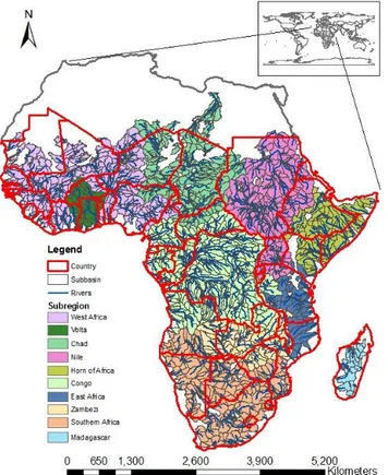
Fig. 1. Study area boundary, sub-region division and watershed
de-lineation in SWAT-SSA model setup.
finer temporal scale (10-day) relative to the typical monthly interval for most GRACE products.
The rest of the paper is organised as follows: the setup of the SWAT model is described in Sect. 2, and the key datasets and steps for calibrating and evaluating the SWAT-SSA mod-els are described in Sect. 3 through 5. Section 6 presents the results of the model calibration and validation. A summary of the major findings from this study and their implications are provided in Sect. 7.
2 SWAT model setup
The model area in this study is ∼ 21 million km2 (Fig. 1).
The major datasets used for the setup or initial parameterisa-tion of the SWAT-SSA model are listed in Table 1. The data acquisition and processing strategy in our study are similar to those described in Schuol et al. (2008a, b), but updated data or alternative options were selected in most cases.
The drainage topology of the study region is represented in SWAT by partitioning the river basins into subbasins and defining the corresponding drainage network of the river system with one river channel segment in each subbasin. Elevation data used in this step of watershed delineation were clipped from the HydroSHEDS database (Lehner et al., 2008). HydroSHEDS is a derivative mapping product
Table 1. The datasets for SWAT model setup.
Category Source Elevation HydroSHEDS
Soil Harmonized world soil database (HWSD)
Land cover Global land cover (GLC) 2000 Lakes & reservoirs Global lake and wetland database
(GLWD)
Climate Precipitation: Global Precipita-tion Climate Project (GPCP) Temperature and relative humid-ity: Goddard Earth Observing System model version 4 and ver-sion 5 (GEOS-4 & GEOS-5) Solar radiation: Release 3 of the NASA/GEWEX Surface Radia-tion Budget (GEWEX SRB 3.0) project and NASA’s Fast Long-wave And SHortLong-wave Radiative Fluxes (FLASHFlux) project
from NASA’s 3 arc-second (approximately 90 m in equato-rial area) SRTM (Shuttle Radar Topography Mission) eleva-tion data and is the best currently available (with highest res-olution) hydrologically conditioned digital elevation dataset for SSA. Based on topographic analysis of HydroSHEDS el-evation data, SSA was divided into 1488 subbasins (Fig. 1). Furthermore, SWAT is a semi-distributed watershed model with potentially different parameter values for different sub-basins/reaches. To reflect the spatial variability of SWAT pa-rameters in calibration and considering computational ef-ficiency, the SSA was divided into 10 sub-continental re-gions; one SWAT model was set up and calibrated separately for each sub-continental region (Fig. 1; Table 2).
Within a subbasin, SWAT allows multiple hydrologic response units (HRUs) to be defined that reflect spatial variability in soil and land cover distributions. However, due to computational limitations, only one HRU with the dominant land cover and soil was created for each sub-basin (Winchell et al., 2007). The soil data were ob-tained from the Harmonized World Soil Database (HWSD, v. 1.1, FAO/IIASA/ISRIC/ISSCAS/JRC, 2009) and the land cover data were obtained from the Global Land Cover 2000 database (European Commission, Joint Re-search Centre, 2003, http://bioval.jrc.ec.europa.eu/products/ glc2000/glc2000.php). The HWSD contains updated soil data for eastern, central and southern African countries rel-ative to the FAO/UNESCO Soil Map of the World. The soil attribute data in HWSD meet most requirements for SWAT model parameterisation; however, two important pa-rameters that describe the hydrologic properties of soils
3086 H. Xie et al.: Semi-distributed watershed model of Sub-Saharan Africa using GRACE data
Table 2. Sub-regions in SWAT-SSA model setup and calibration.
Area Area
Name (×103km2) Name (×103km2)
West Africa 3550 Congo 4474 Volta 534 Eastern Africa 808 Chad 2576 Southern Africa 2928 Nile 2841 Zambezi 1365 Horn of Africa 1477 Madagascar 309 Total: 20 862
(available water capacity and saturated hydraulic conduc-tivity) are missing and were estimated using pedotransfer functions (Saxton et al., 1986; Schaap et al., 2001).
Climate forcing data for SWAT include 1 degree daily (1DD) precipitation, temperature, solar radiation and rel-ative humidity data and were obtained from the NASA Langley Research Center POWER Project. A GIS layer of polygon-based SWAT subbasin boundaries was overlaid with a GIS layer of climate gridded data to calculate frac-tions of area covered by different climate data grid cells for each subbasin and to compute area-weighted values of climatic variables as basin-wide estimates of these vari-ables. The original source of the precipitation data is the Global Precipitation Climate Project (GPCP, http://precip. gsfc.nasa.gov). The 1-DD GPCP dataset combined obser-vations from multiple sensors (Huffman et al., 2001). The data for other climate variables were compiled from various NASA’s projects (Table 1) by the POWER project and were primarily used for estimation of potential evapotranspiration (PET). SWAT includes three different methods for estimating PET (Neitsch et al., 2005) with varying data requirements and the Priestley-Taylor method (Priestley and Taylor, 1972) was selected because it is considered more accurate than the Hargreaves method (Hargreaves and Samani, 1985), which is temperature-based, and reliable estimates of wind speed required for the Penman-Monteith method (Monteith, 1965) were not available at the time of this study.
SWAT also provides two options for simulating flow rout-ing in river channels. The variable storage method was used to route water in river channels because pilot simulations suggested that this is more robust than the Muskingum option in this study. Anthropogenic impacts on water resources were considered to be negligible in SSA. Agriculture is the domi-nant water use sector. However, current agriculture in SSA is mainly rainfed; the area of SSA equipped for irrigation only accounts for 3 % of the total cultivated area (Siebert, 2010; FAO, 2011). Therefore, existing irrigation was not simulated in this study.
SSA has a number of large fresh water bodies, such as Lake Victoria, the world’s second largest fresh water lake in terms of surface area (239 000 km2), and Lake Volta, the world’s largest reservoir in terms of surface area (8502 km2).
38 815
816
Figure 2 Global Runoff Data Centre (GRDC) stations and reservoirs/lakes included in the 817
SWAT-SSA model setup and calibration (lengths of GRDC discharge data series are marked 818
with missing values excluded) 819
820 821
Fig. 2. Global Runoff Data Centre (GRDC) stations and
reser-voirs/lakes included in the SWAT-SSA model setup and calibration (lengths of GRDC discharge data series are marked with missing values excluded).
The major lakes and reservoirs in SSA were defined in our SWAT-SSA model (Fig. 2). Locations and storage capaci-ties of these water impoundments were obtained from the Global Lakes and Wetlands Database (GLWD) (Lehner and D¨oll, 2004). Due to signal leakage, mass variations in these lakes and reservoirs may have a significant contribution to GRACE TWS observations (e.g., Becker et al., 2010), even if their size is much less than the GRACE footprint (∼ 450 km,
i.e., 200 000 km2in area). We compared the simulated water
level change data and water level change data obtained with satellite altimetry (Cr´etaux et al., 2011, see http://www.legos. obs-mip.fr/en/soa/hydrologie/hydroweb/) and found that it is difficult to adequately simulate water storage variations in these lakes and reservoirs because of lack of detailed bathymetry and reservoir operation data. In this study, an al-ternative modelling strategy was taken, i.e., lake and reser-voir mass correction was applied to GRACE TWS data ac-cording to height and volume variations of the 22 largest lakes and reservoirs in SSA (Table 3) from satellite altime-try data analysis for a fair comparison between GRACE and hydrologic model. Accordingly, simulated water mass varia-tions in lakes and reservoirs were excluded from the model-based TWS variation calculation.
Table 3. Lakes/reservoirs to which mass corrections in GRACE data processing were applied.
1. Albert 6. Kainji 11. Malawi 17. Tana 22. Volta 2. Bangweulu 7. Kariba 12. Mweru 18. Tanganyika
3. Buyo 8. KhashmGirba 13. Nasser 19. Chad 4. CahoraBassa 9. Kivu 15. Roseires 20. Turkana 5. Edward 10. Kyoga 16. Rukwa 21. Victoria
Table 4. SWAT hydrologic calibration parameters.
Parameter Level Possible range
CN2: SCS curve number HRU/subbasin 35 ∼ 90
ESCO: Soil evaporation compensation factor Basin 0 ∼ 1
GW DELAY: Groundwater delay coefficient [days] HRU/subbasin 0 ∼ 100
GW REVAP: Groundwater revap coefficient HRU/subbasin 0.02 ∼ 0.2
ALPHA BF: Baseflow alpha factor [days] HRU/subbasin 0 ∼ 1
REVAPMN: Threshold depth to water in the shallow aquifer for “revap” to occur [mm]
HRU/subbasin 0 ∼ 500
GWQMN: Threshold depth to water in the shallow aquifer required for groundwater flow to occur [mm H2O]
HRU/subbasin 0 ∼ 1000
SURLAG: Surface runoff lag coefficient Subbasin 1 ∼ 10
SOL AWC Xa: Calibration factor for soil water available capacity Soil layer/subbasin 0.5 ∼ 2
SOL D Xa: Calibration factor for depth from soil surface to bottom of layer
Soil layer/sbubasin 1 ∼ 2
SOL K Xa: Calibration factor for saturated hydraulic conductivity
Soil layer/sbubasin 0.5 ∼ 1.5
aThese factors are defined for model calibration purposes only. Actual values of these parameters used in simulation are equal to their default values multiplied by the calibration factors.
3 GRACE data
GRACE data used in this study were obtained from CNES-GRGS (Centre National d’Etudes Spatiales-Groupe de Recherches de G´eod´esie Spatiale), RL2 product (Bru-insma et al., 2010). The data are provided as spherical har-monics as 10 day means. The Stokes coefficients are trun-cated at degree 50 to remove high frequency noise. No fur-ther filtering is required for these solutions. Stokes coeffi-cients were recombined following Wahr et al. (1998) and pro-jected on a 0.5°latitude/longitude grid. In terms of time frame of the data, we used 232 10-d periods from 29 July 2002 through 22 April 2009 (with missing values from 26 Novem-ber 2002 to 23 February 2003, 25 May 2003 to 3 July 2003, and 20 January 2004 to 29 January 2004).
The GRACE CSR RL04 product (Center for Space Re-search, University of Texas at Austin, monthly timescales, Bettadpur, 2007) was also used to estimate GRACE errors at a 10-day timescale. CSR data were destriped according to Swenson and Wahr (2006). For error calculation, both GRGS and CSR GRACE products were truncated at degree 30 and smoothed using a 300-km Gaussian smoother to eval-uate large-scale errors. Error is computed at a monthly time step as the difference between CSR and GRGS data and re-sampled as 10-day errors.
In the mass correction, the impact of 22 lakes and reser-voirs were first forward modelled at GRACE GRGS resolu-tion, prior to subtraction from GRACE. Lake volume vari-ations were distributed on a grid and projected on spherical harmonics. They were then recombined up to degree 50 on a 0.5 degree grid.
4 Total water storage variation calculation in SWAT
SWAT was developed to provide continuous simulations of the basin hydrology at a daily timescale. For each day of the simulation, the model first computes the water yields on land and then routes the water through the defined river channel network. In the land phase simulation, SWAT uses the Soil Conservation Service (SCS) curve number method (SCS 1972) to estimate the volume of overland flow and storage routing techniques to simulate percolation and lat-eral movement of water through the soil profile. The water leaving the base of the soil profile does not enter aquifers im-mediately, but is time lagged based on transport through the vadose zone. The vadose zone is defined in SWAT as the un-saturated zone beneath the base of the soil profile and above the groundwater table. An exponential decay weighting func-tion, proposed by Venetis (1969), was used to account for the time delay of water drainage in the vadose zone and to
3088 H. Xie et al.: Semi-distributed watershed model of Sub-Saharan Africa using GRACE data 39 822 823 824 825 40 826 827
Figure 3 The Pareto fronts in objective space
828 829
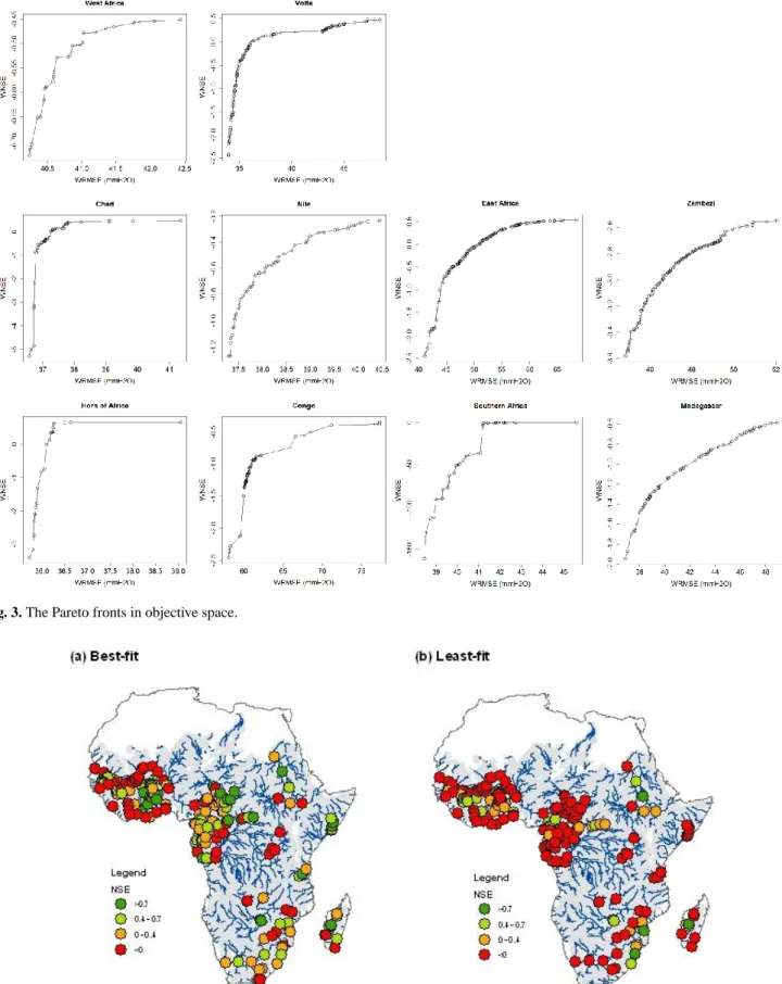
Fig. 3. The Pareto fronts in objective space.
41 830
Figure 4 Model fit in river discharge simulations
831 832 833 834
Fig. 4. Model fit in river discharge simulations.
Table 5. Nash-Sutcliffe efficiency coefficients for calibrated SWAT models for simulation of variations in TWS.
Calibration Validation Mean Max. Min. Mean Max. Min. West Africa 0.91 0.92 0.89 0.91 0.92 0.90 Volta 0.86 0.90 0.75 0.91 0.94 0.82 Chad 0.81 0.83 0.79 0.66 0.73 0.55 Nile 0.86 0.87 0.84 0.75 0.78 0.72 Horn of Africa 0.41 0.45 0.40 0.31 0.34 0.25 Congo 0.19 0.34 −0.44 0.12 0.30 −0.80 Eastern Africa 0.85 0.91 0.71 0.80 0.87 0.67 Zambezi 0.91 0.92 0.90 0.91 0.93 0.89 South Africa 0.46 0.54 0.40 0.80 0.83 0.75 Madagascar 0.81 0.85 0.76 0.82 0.84 0.79
predict effective recharge into shallow aquifers (Sangrey et al., 1984). Variation in groundwater flow to rivers is linearly related to changes in water-table elevation.
SWAT simulates several water storage components that make up total water storage to compare with GRACE TWS. These storages include:
1. Overland water storage (V1), including river
chan-nels, bank storage and canopy storage. Due to the mass correction in GRACE data processing, the wa-ter storage variations in lakes/reservoirs were not taken into account.
2. Storages (V2+V3)for lagged surface runoff and lateral flow. The two storages are defined in SWAT for esti-mating the amount of overland and lateral flow reaching river channels on a daily time step. SWAT allows for de-layed release of overland flow and lateral flow yielded in river basins with time of concentration greater than one day.
3. Soil profile (V4).
4. Vadose zone (V5). Water storage in the vadose zone is
typically not considered as a storage in SWAT water balance analysis because the Venetis’ exponential decay weighting function (1969) does not alter the quantity of water from soil into aquifers. However, the time delay for water to move through the vadose zone results in variations in water storage and needs to be addressed in TWS variation calculations (Milzow et al., 2011).
5. Groundwater (V6). SWAT simulates an unconfined
shal-low aquifer and a confined deep aquifer in each sub-basin. Water storage in shallow aquifers may contribute to flow in the main river channels or be re-evaporated into the soil. By contrast, there is no simulated outlet for water in deep aquifers except pumpage. “Water that en-ters the deep aquifer is assumed to contribute to stream-flow somewhere outside of the watershed” (Neitsch et
al., 2005). While this assumption may hold in studies for small river basins, it is no longer valid at a continen-tal scale. Due to the accumulation of water percolated from shallow aquifer, an upward trend in water storage in deep aquifers would be found, which is unrealistic. To circumvent this problem, the deep aquifer was excluded from the simulations and the calculation of TWS by set-ting the percolation rate to the deep aquifer to zero. For each subbasin, the model-based TWS for each 10-day period was calculated as:
TWSt =V1,t+V2,t+V3,t+V4,t+V5,t+V6,t
where t is the index for the 10-day period. The series of
SWAT subbasin-wide TWS anomalies (TWSVt)was
com-puted by differencing the TWS for each 10-day period TWSt
and the mean of the TWS over the entire GRACE data period:
TWSVt=TWSt−TWS
where TWS is the mean of the TWSt over the GRACE
data period, or was calculated by taking the average of
10-d TWSt’s during July 2002–April 2009.
5 Calibration approach
Calibration and evaluation of the SWAT-SSA model in this study was carried out using a multi-criteria framework, sim-ilar to the studies by Werth and G¨untner (2010). The multi-criteria approach extends the traditional calibration approach by casting the calibration into a multi-objective optimisa-tion problem, and for independent data, allows evaluaoptimisa-tion of model performance against more than one objective to improve model robustness and predictability (Gupta et al., 1998). The solution to the multi-criteria optimisation pro-gramme consists of the non-dominated calibration parame-ter sets, which are optimal in a Pareto efficiency sense. The trade-off between model fits evaluated by different criteria
3090 H. Xie et al.: Semi-distributed watershed model of Sub-Saharan Africa using GRACE data 42 835 836 837 43 838 839 840
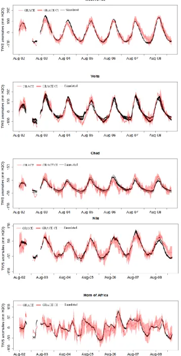
Fig. 5. Observed and zonally averaged simulated TWS
varia-tions for ten sub-continental regions (TWS-total water storage; CI-confidence).
reflects the minimum parameter uncertainty (Vrugt et al., 2003) caused by errors in the input and measured data as well as by the model structure.
For the calibration of the SWAT-SSA model, two objective functions were defined. Their definitions and calculations are explained in detail below. The multi-objective optimisa-tion problems defined in the multi-criteria calibraoptimisa-tion of the SWAT-SSA models were solved using the Non-dominated Sorting Genetic Algorithm II (NSGA-II, Deb et al., 2002),
43 838 839 840 44 841 842 843 45 844
Figure 5 Observed and zonally averaged simulated TWS variations for ten sub-continental
845
regions (TWS-total water storage; CI-confidence)
846
Fig. 5. Continued.
a population-based heuristic evolutionary optimisation tech-nique with a proven track record of success in solving many large-scale optimisation problems. The population sizes cho-sen in the optimisations varied from 150 to 300, and the opti-misations lasted for 50 ∼ 100 generations until no significant improvements in the solution were observed.
5.1 Comparison of model-based and GRACE-derived
TWS variations
As GRACE provides a filtered image of reality, the mod-elled storage variations from SWAT were first converted to GRACE resolution to provide storage values at the same
46
(a) Best-fit (b) Least-fit
847
848
(c) Agro-climatic zonation (d) Cropland intensity
849
850
Figure 6. Spatial patterns of SWAT model fits in simulations of total water storage variations in
851
Sub-Saharan Africa (country boundaries are shown).
852
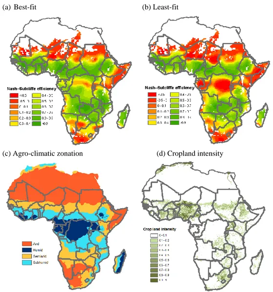
Fig. 6. Spatial patterns of SWAT model fits in simulations of total water storage variations in Sub-Saharan Africa (country boundaries are
shown).
spatial scales for comparison. This mathematical process in-volves projecting SWAT modelled spatial fields to Spher-ical Harmonics (SH) up to degree 50 (in this study, SH transformation was conducted using SHTOOLS, http://www.
ipgp.fr/∼wieczor/SHTOOLS/SHTOOLS.html) in which the
SWAT-based basin-wide TWS variations for each 10-day pe-riod were first disaggregated into a 0.5 by 0.5 degree grid prior to the transformation. In order to allow for a compari-son between GRACE- and SWAT-based TWS variations for sub-continental regions, simulated variations in TWS by the Noah land surface model (Ek et al., 2003) in NASA’s Global Land Data Assimilation System (GLDAS) (Rodell et al., 2004) were used as a priori information to fill areas outside of the SSA sub-region of interest in the SH transformation.
Agreement between GRACE-derived and model-based TWS variations was evaluated using a weighted total square
error (WTSE) function:
WTSE = T X t =1 I X i=1 J X j Is×wi,j,t
×(TWSVi,j,t,SWAT−TWSVi,j,t,GRACE)2 (1)
where TWSVi,j,t,SWATand TWSVi,j,t,GRACEare SWAT- and
GRACE-based TWS variations for 10-day period t and grid cell (i, j ), respectively. Is is an indicator function. Is=1 if the grid cell is located within the study region; otherwise,
Is=0, wi,j,t is the weight, an inverse of standard error of
GRACE-based TWS variations TWSVi,j,t,GRACE.
Finally, following the convention in hydrologic model calibration, available GRACE data were divided into two groups: the first 112 10-day periods (29 July 2002– December 2005) were used for calibration and the data for remaining 120 10-day periods were reserved for validation.
3092 H. Xie et al.: Semi-distributed watershed model of Sub-Saharan Africa using GRACE data
Table 6. Temporal variability of zonally averaged component-wise water storage variations (%).
West Horn of Eastern South
Africa Volta Chad Nile Africa Congo Africa Zambezi Africa Madagascar
Soil Mean 55.2 11.5 31.5 37.9 44.8 10.0 28.8 18.9 20.8 9.1 Max 61.1 16.2 58.5 48.9 48.8 31.0 38.9 21.4 38.5 13.8 Min 50.3 8.5 20.8 31.4 37.0 5.3 17.1 17.4 8.6 6.8 Vadose Mean 5.2 46.7 26.9 4.5 9.8 37.1 19.4 16.8 13.9 42.6 Max 9.5 55.0 34.2 11.6 13.1 51.5 31.0 19.8 40.8 59.2 Min 2.7 8.1 3.0 0.0 6.0 0.24 0.0 12.5 3.1 21.6 Groundwater Mean 1.6 15.3 6.2 13.0 11.3 8.4 5.1 8.4 25.3 2.9 Max 3.6 56.4 24.8 24.5 16.2 59.1 25.5 16.2 41.5 8.6 Min 0.42 5.3 2.0 6.7 8.1 0.01 2.7 6.6 11.5 0.08 Overland water Mean 0.03 0.04 0.01 0.4 0.007 0.10 0.004 0.010 0.03 0.0004 Max 0.05 0.10 0.02 0.58 0.009 0.30 0.010 0.020 0.06 0.0010 Min 0.02 0.01 0.01 0.25 0.006 0.01 0.002 0.005 0.01 0.0002
Surface water lag
Mean 0.003 0.20 0.07 0.03 0.01 0.06 0.01 0.22 0.31 0.02 Max 0.005 1.23 0.52 0.14 0.01 0.32 0.02 0.59 0.83 0.03 Min 0.002 0.001 0.003 0.005 0.01 0.03 0.002 0.04 0.02 0.01
Lateral flow lag
Mean 0.0007 0.0001 0.00006 0.004 0.0014 0.010 0.005 0.00042 0.0009 0.011 Max 0.0010 0.0002 0.0001 0.04 0.0015 0.020 0.030 0.0010 0.0015 0.030 Min 0.0004 0.00006 0.00004 0.001 0.0013 0.001 0.001 0.00036 0.0005 0.006
5.2 Criterion/objective function for evaluating goodness
of model fit in runoff field simulation
Observed monthly river discharge data from 187 discharge stations in SSA (Fig. 2) were used for this calibration study. The data were obtained from Global Runoff Data Centre (GRDC), a primary source of information for global river discharge to support large-scale hydrologic studies (date of data retrieval: 30 September 2009). The starting and ending dates of the discharge series for these stations vary by station. The earliest discharge data date back to 1900 and were ob-tained from the station near Khartoum on the Blue Nile River. The most recent data are from 2001 and several stations on the Orange River, the Great Fish River and the Limpopo River in South Africa. For the majority of stations in SSA, river discharge data are available up to 1980s and early 1990s. The different time frames among the GRDC river discharge data, GRACE data (2002–2009), and GPCP 1-DD precipitation data (1997–2009) pose difficulty for model cal-ibration. In this study, we focused on evaluating the per-formance of SWAT for modelling TWS variability: SWAT was run for 2002–2009 (with five additional years 1997– 2001 as the spin-up period) and, following the approach by Werth and G¨untner (2010), simulated and observed monthly river discharge rates in two time frames were compared on a multi-year average basis. The fit of the SWAT model at each GRDC station was measured using the Nash-Sutcliffe Effi-ciency (NSE) coefficient (Nash and Sutcliffe, 1970), which
is defined as NSE = 1 − 12 P t =1 (Qt,obs−Qt,sim)2 12 P t =1 (Qt,obs− ¯Qt,obs)2 (2)
where Qt,obsand Qt,simare the multi-year averaged monthly discharges calculated using the simulated and available ob-served discharges (m3s−1), respectively. ¯Qt,obsis the mean of Qt,obs(m3s−1). The NSE coefficient can range from −∞ to 1, where 1 indicates a perfect model fit.
The GRDC station network is relatively dense in West Africa, but limited in other regions (Fig. 2). This highlights the benefit of applying GRACE data to support hydrologic simulations in SSA. The NSE values for all GRDC stations in a sub-regional model were weighted by length of observed monthly river discharge series:
WNSE =X
i
wi NSEi (3)
where NSEi is NSE coefficient at GRDC station i, and wiis
the weighting factor proportional to the length of the monthly
river discharge data time series at that station (P
i
wi =1).
The weighted NSE (WNSE) serves as the criterion for eval-uating performance of SWAT in simulating river discharge.
H. Xie et al.: Semi-distributed watershed model of Sub-Saharan Africa using GRACE data 3093 47 853 854 855 48 856 857 858
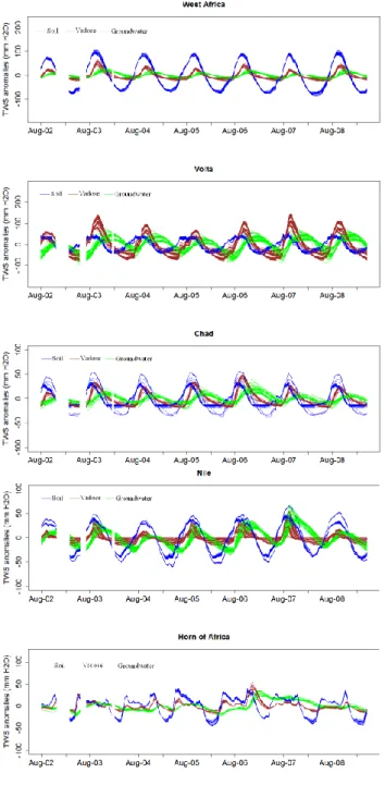
Fig. 7. Zonally averaged water variations in soil, vadose zone and
groundwater storages (TWS-total water storage).
5.3 Calibration parameters
The hydrologic processes and watershed properties in SWAT are characterised by many parameters. A list of SWAT pa-rameters selected for calibration, together with their lower and upper bounds of adjustable ranges, are shown in Table 4. This list was determined from literature review, numerical sensitivity analysis (Morris, 1991), and according to results from several test runs of the calibration programmes.
48 857 858 49 859 860 861 862
Figure 7 Zonally averaged water variations in soil, vadose zone, and groundwater storages
863
(TWS-total water storage)
864
Fig. 7. Continued.
In these SWAT calibration parameters, SCS curve num-ber is a key parameter for surface runoff estimation. It is defined to characterise the potential maximum soil mois-ture retention capacity. A low value indicates low runoff, but high infiltration potential. Surface runoff lag coefficient (SURLAG) determines how much total available runoff en-ters into a river reach on a given day and is a sensitivity parameter for simulating river discharge hydrographs. Soil evaporation compensation factor (ESCO) is defined to spec-ify the depth distribution used to meet soil evaporative de-mand. As the value of ESCO decreases, more water can be evaporated from deeper soil layers. SOL AWC, SOL K, and
3094 H. Xie et al.: Semi-distributed watershed model of Sub-Saharan Africa using GRACE data 51 865 866 867 52 868 869 870
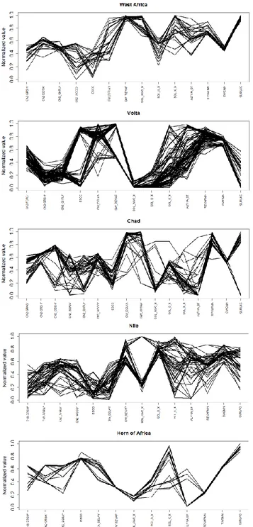
Fig. 8. Estimates of SWAT calibration parameters obtained from
mutli-criteria calibration (abbreviations of the land cover type: FOCD – Closed deciduous forest; FORC – Closed evergreen low-land forest; FORD – Degraded evergreen lowlow-land forest; FORS – Submontane forest; GRAS – Closed grassland; GRSH – Open grassland with sparse shrubs; ODSH – Open deciduous shrubland; OGRA – Open grassland; SAVA – Mosaic Forest/Savanna; SGRA – Sparse grassland; SHRU – Deciduous shrubland with sparse trees; WOOD – Deciduous woodland).
52 868 869 870 53 871 872 873 54 874
Figure 8 Estimates of SWAT calibration parameters obtained from mutli-criteria calibration
875
(abbreviations of the land cover type: FOCD-Closed deciduous forest; FORC-Closed evergreen
876
lowland forest; FORD-Degraded evergreen lowland forest; FORS-Submontane forest;
GRAS-877
Closed grassland; GRSH-Open grassland with sparse shrubs; ODSH-Open deciduous shrubland;
878
OGRA-Open grassland; SAVA-Mosaic Forest / Savanna; SGRA-Sparse grassland;
SHRU-879
Deciduous shrubland with sparse trees; WOOD-Deciduous woodland)
880
Fig. 8. Continued.
SOL D are soil available water capacity, saturated conduc-tivity and the soil layer depth, respectively. All three soil at-tributes are highly uncertain. Values of the first two param-eters were derived using pedotransfer functions; no reliable information about the actual depth of the soil layer in Africa is available from HWSD, only a reference value (in most cases 1 m) was assigned. GW DELAY (groundwater delay coefficient) characterising the delay time for recharge into the aquifer, is a single controlling parameter for determining
the water storage variation in the vadose zone. The remain-ing four parameters in the table, GW REVAP (groundwater revap coefficient), ALPHA BF (baseflow alpha factor), RE-VAPMN (threshold depth of water in the shallow aquifer for “revap” to occur) and GWQMN (threshold depth of water in the shallow aquifer required for groundwater flow to occur) control the behaviour of shallow aquifers.
The ten SWAT sub-regional models were calibrated with the parameters shown in Table 4. The model for each sub-region was calibrated independently, but within a sub-region, the same percentage changes were made for those parame-ters which have spatially varying values (or parameparame-ters other than SURLAG and ESCO), except for the SCS curve number (CN2), based on spatial fields of their initial estimates. The CN2 values are correlated with land cover and soil perme-ability. In this study, within a sub-region the CN2 parameters were grouped by land cover, and the CN2 values for major land covers/uses were considered as independent calibration parameters.
6 Results
The Pareto fronts in the two-dimensional objective space found via multi-criteria calibration for all ten SSA sub-regions are shown in Fig. 3. Paired values of weighted root-mean-square-error (RMSE) and weighted NSE coeffi-cients are plotted on horizontal and vertical axes, respectively (weighted RMSE is a monotonic function of weighted TSE). A model with a perfect fit to GRACE data and river discharge data would have a weighted RMSE of 0 and a weighted NSE coefficient of 1. Thus, the Pareto front curves are convex to-wards the point (0, 1), reflecting tradeoffs between the ability to fully describe discharge or TWS variations.
With regard to performance of calibrated models in river discharge simulation, the highest values of weighted NSE co-efficients obtained vary from −2.55 to 0.66 and are negative for five out of the ten sub-region models (West Africa, Nile, Congo, Zambezi and Madagascar). This measure of good-ness of fit statistic is also sensitive to different solutions of parameter sets in Pareto fronts. The deterioration of its value is greater than two in models for all sub-regions other than West Africa, Nile and Zambezi when the parameter set in the Pareto frontier that most closely matches the simulation of GRACE TWS variations was used. The NSE model coeffi-cients for each individual GRDC gauging station are shown in Fig. 4. When the “best-fit” solutions for river discharge simulation were taken, 20 % of the stations have NSEs ≥ 0.7, 43 % ≥ 0.4 and the NSEs for 64 % of the GRDC stations are positive. These percentages decrease from 20 to 6 %, 43 to 17 % and 64 to 30 % if the models are run with the “least-fit” solutions for river discharge simulation.
More satisfactory model fits were achieved in simulation of TWS variations after the calibration of the SWAT model. The ensembles of time series of zonally averaged simulated
TWS variations over the 10 sub-regions and associated with Pareto optimal solutions found in multi-criteria calibration are plotted in Fig. 5, together with the time series of zonally averaged GRACE- based mean TWS variations and the re-lated one-sigma (68.7 %) confidence interval (CI). The NSE coefficients for the time series of model-based TWS tions with respect to the GRACE- based mean TWS varia-tions were also calculated and summarised, for calibration and validation periods, respectively (Table 5). Overall, sim-ulated and GRACE-based zonally averaged time series are in good agreement in sub-regions of West Africa, Volta, Chad, Nile, Eastern African, Zambezi and Madagascar dur-ing both calibration and validation periods. The means of the NSE coefficients for these sub-regional models range from 0.66 to 0.91. Larger discrepancies were found in the Congo and Horn of Africa. In the simulation of temporal variations of TWS for these two sub-regions, the model still captures the general trends/phase changes of TWS variations, but the mismatch in amplitude is greater. For the Southern African model, the model fit was poorer during the calibration pe-riod; however, the model performs much better during the validation period.
The NSE coefficients calculated on a gridded basis are shown in Fig. 6a and b. The “best-fit” and “least-fit” solu-tions were determined according to model fits with respect to GRACE TWS variations. Figure 6c and d show the agro-climatic zonation (derived from FAO Agroecological Zones crafted by HarvestChoice, Z. Guo, personal communication, 2011), and the density of cropland (fraction of cropland area in 5 min × 5 min grid, Ramankutty et al., 2008) in SSA. Gen-erally, the model performs well in simulating TWS varia-tions in semiarid and sub-humid areas, which encompass most cropland in SSA. The largest discrepancies in simulated TWS variations (NSE coefficients ≤ 0) occurred in arid ar-eas, where water storage amplitude is lower or equivalent to GRACE error (the Sahara, Somalia, western Ethiopia, north-west Kenya, south Namibia and most of Southern Africa) and the equatorial humid area (notably in central Democratic Re-public of the Congo).
GRACE TWS data integrate water mass variations from all storage components. Sometimes, interest is focused on es-timating water mass variations in certain storage components (e.g., groundwater; Rodell et al., 2009; Tiwari et al., 2009). Temporal variability of zonally aggregated water mass in six water storages parameterised in the SWAT model are charac-terised by calculating ratios between variances of these stor-age variables σV2
i( i = 1, · · · , 6) and variance of model-based total water storage variation σV2
Total (in unfiltered space), or
σV2
i
. σV2
Total. Means and ranges of calculated normalised
vari-ances for each storage variable and each sub-region are listed in Table 6 (note that the water mass variations in six stor-ages are not independent; thus, σV2
Totalmay not equal
6
P
i=1
σV2
i). These statistics show that the three water storage components
3096 H. Xie et al.: Semi-distributed watershed model of Sub-Saharan Africa using GRACE data that have largest temporal variability, thus, contributing most
to TWS, are soil, vadose zone and groundwater storage. By contrast, contributions from overland flow, surface runoff and lateral flow lags are trivial. Zonally aggregated time series of soil water, vadose zone water and groundwater storage vari-ations obtained from the calibrated SWAT models are shown in Fig. 7. Systematic phase differences exist among the time series for the three storage variables: in each annual cycle when the rainy season begins the soil moisture is first replen-ished and peaks, followed by vadose zone water and then groundwater.
The statistics in Table 6 and graphs in Fig. 7 also indicate that there could be even larger uncertainties in estimation of component-wise water storages than what is seen in TWS es-timation. For example, the model gives divergent estimates for water storage variations in vadose zone and groundwater in Eastern Africa when the model was run with parameter sets across the Pareto frontier. The estimated time series for water storage variations in the vadose zone and groundwa-ter fall into two groups: one group has large variations in the vadose zone water storage, but relatively smaller variations in groundwater storage; in another group, vadose zone water storage variations are almost zero and variations in ground-water storage are much larger. Figure 8 shows the Pareto fronts in parameter space with normalised parameter values in [0, 1] intervals (zero values represent the lower bounds of the adjustable ranges of the parameters and one corresponds to the upper bounds). The disparate estimates for vadose zone and groundwater storage variations can be explained by the dichotomy in the estimated values of GW DELAY. As the value of GW DELAY approaches zero, water exiting the bot-tom of the soil profile can enter aquifers immediately caus-ing no variation in vadose water storage and larger variations in groundwater storage, with the opposite for large values for GW DELAY. Similar divergent estimates in vadose zone water and groundwater storage variations caused by different GW DELAY estimates were also found in the Congo model. For Chad, Nile and Southern Africa, there are large uncer-tainties in estimating soil water storages, which is most likely related to divergent estimates of SOL AWC X.
7 Discussion and conclusions
The study presented in this paper concerns calibra-tion/evaluation of a semi-distributed model based on SWAT code (SWAT-SSA) for regional-scale hydrologic simulation in Sub-Saharan African countries. The SWAT-SSA models were calibrated and evaluated in a multi-criteria framework to both river discharge and GRACE TWS data, but with more focus on assessing the model’s capacity for simulating TWS variability using GRACE data. In spite of uncertainty aris-ing from the tradeoff in optimisaris-ing model parameters with respect to two model fitting criteria and in estimation of stor-age variations contributed by different storstor-age components,
the study showed that the calibrated SWAT-SSA model per-forms well in simulating TWS variations in semi-arid and semi-humid areas, where agriculture in SSA is concentrated and, therefore, is capable of acting as an effective modelling tool for agricultural water management in SSA.
Any model calibration and validation exercise is subject to certain limitations. A major limitation in this study origi-nated from use of multi-year average monthly river discharge data for a time frame (1900–2001) different from that in which the models were actually run (2002–2009) as a re-sult of limited availability and accessibility to recent stream flow data in Sub-Saharan countries. Therefore, it is difficult to evaluate the model’s adequacy in simulating the surface water system. Climate and land use change may alter the flow regimes of rivers (e.g., Amogu et al., 2010) and poten-tially bias the calibration of river discharge and estimation of the contribution of water mass variations in river systems to TWS variations. Furthermore, an interesting question of-ten raised in model calibration/evaluation is what value is brought to model calibration and evaluation by use of ad-ditional dataset(s). The limitation with river discharge data makes it difficult to answer this question. However, the out-come of the SWAT model calibration and validation in this study tends to suggest that use of GRACE data may only provide limited additional constraints to reduce parametric uncertainties of the model because the NSEs shown in Fig. 3 and Table 5 indicate that there might be stronger equifinal-ity (Beven and Binley, 1992) in the TWS simulation than in discharge simulation. On the other hand, it is apparent that GRACE data are of great value in that they provide valuable information and unprecedented opportunity to validate and evaluate the model’s capacity to simulate spatio-temporal variability in TWS.
Finally, there is less agreement between model- and GRACE-based TWS variations in arid and equatorial hu-mid areas. A few possible reasons for the larger discrepan-cies include: firstly, uncertainties associated with GRACE TWS variations themselves. Noticeable disagreement be-tween model- and GRACE-based TWS variations in arid regions were also reported by Ngo-Duc et al. (2007) in a global-scale model validation study, who attributed the dis-agreements in arid areas to weak GRACE signals and result-ing larger errors in GRACE TWS variations. Secondly, er-rors in climatic forcing data, especially in precipitation data may be important. Due to lack of ground-based observations in precipitation, regional or global scale hydrologic simula-tions typically rely on use of precipitation estimates from dif-ferent satellite-based or meteorological reanalysis data prod-ucts. Uncertainty associated with these precipitation datasets is often a principle source of uncertainty for hydrologic sim-ulation (e.g., Fiedler and D¨oll, 2007). Thirdly, inadequacy of SWAT parameterisation or algorithms in simulating hydrol-ogy in arid and humid areas may also help explain the dis-crepancy. Future work will be required to identify physical reasons for model misfits and for model enhancement.
Acknowledgements. This study was funded by a grant from the
Bill & Melinda Gates Foundation. The findings and conclusions contained within are those of the authors and do not necessarily reflect positions or policies of the Bill & Melinda Gates Foundation. The meteorological data were obtained from the NASA Langley Research Center POWER Project funded through the NASA Earth Science Directorate Applied Science Program. Additional support was provided to L. Longuevergne and B. R. Scanlon through the Jackson School of Geosciences.
Edited by: E. Morin
References
Alkama, R., Decharme, B., Douville, H., Becker, M., Cazenave, A., Sheffield, J., Voldoire, A., Tyteca, S., and Le Moigne, P.: Global Evaluation of the ISBA-TRIP Continental Hydrological System. Part I: Comparison to GRACE Terrestrial Water Storage Esti-mates and In Situ River Discharges, J. Hydrometeorol., 11, 583– 600, 2010.
Amogu, O., Descroix, L., Y´ero, K. S., LeBreton, E., Mamadou, I., Ali, A., Vischel, T., Bader, J. C., Moussa, I. B., Gautier, E., Boubkraoui, S., and Belleudy, P.: Increasing River Flows in the Sahel?, Water, 2, 170–199, 2010.
Arnold, J. G., Srinivasin, R., Muttiah, R. S., and Williams, J. R.: Large Area Hydrologic Modeling and Assessment: Part I. Model Development, Journal of American Water Resources Associa-tion, 34, 73–89, 1998.
Becker, M., Llovel, W., Cazenave, A., G¨untner, A., and Cr´etaux, J. F.: Recent hydrological behaviour of the East African Great Lakes region inferred from GRACE, satellite altimetry and rain-fall observations, CR Geoscience, 342, 223–233, 2010. Bettadpur, S.: Level-2 Gravity Field Product User Handbook,
GRACE 327–734, The GRACE Project, Center for Space Re-search, University of Texas at Austin, 2007.
Beven, K. J. and Binley, A. M.: The future of distributed models: model calibration and uncertainty prediction, Hydrol. Process., 6, 279–298, 1992.
Bruinsma, S., Lemoine, J. M., Biancale, R., and Vales, N.: CNES/GRGS 10-day gravity field models (release 2) and their evaluation, Adv. Space Res., 45, 587–601, 2010.
Chen, J. L., Wilson, C. R., Tapley, B. D., Longuevergne, L., Yang, Z. L., and Scanlon, B. R.: Recent La Plata basin drought conditions observed by satellite gravimetry, J. Geophys. Res., 115, D22108, doi:10.1029/2010JD014689, 2010.
Cr´etaux, J.-F., Jelinski, W., Calmant, S., Kouraev, A., Vuglinski, V., Berg´e-Nguyen, M., Gennero, M.-C., Nino, F., Abarca Del Rio, R., Cazenave, A., and Maisongrande, P.: SOLS: A lake database to monitor in the Near Real Time water level and storage varia-tions from remote sensing data, Adv. Space Res., 47, 1497–1507, 2011.
Deb, K., Pratap, A., Agarwal, S., and Meyarivan, T.: A fast and eli-tist multiobjective genetic algorithm: NSGA-II, IEEE T. Evolut. Comput., 6, 182–197, 2002.
Dhar, S. and Mazumdar, A.: Hydrological modelling of the Kangsabati river under changed climate scenario: case study in India, Hydrol. Process., 23, 2394–2406, 2009.
Ek, M. B., Mitchell, K. E., Lin, Y., Rogers, E., Grunmann, P., Ko-ren, V., Gayno, G., and Tarpley, J. D.: Implementation of Noah
land surface model advances in the National Centers for Environ-mental Prediction operational mesoscale Eta model, J. Geophys. Res., 108, 8851, doi:10.1029/2002JD003296, 2003.
FAO/IIASA/ISRIC/ISSCAS/JRC: Harmonized World Soil Database (version 1.1), FAO, Rome, Italy and IIASA, Lax-enburg, Austria, 2009.
FAO: The State of Food Insecurity in the World 2010: Addressing Food Insecurity in Protracted Crises, Rome, 2010.
FAO (Food and Agriculture Organization of the United Na-tions): Water Resources Development and Management Service, AQUASTAT database, available at: http://www.fao.org/nr/water/ aquastat/dbases/index.stm, last access: July, 2011.
Falkenmark, M. and Rockstrom, J.: The New Blue and Green Water Paradigm: Breaking New Ground for Water Resources Planning and Management, J. Water Res. Pl. ASCE, 132, 129–132, 2006. Famiglietti, J. S., Lo, M., Ho, S. L., Bethune, J., Anderson, K. J., Syed, T. H., Swenson, S. C., de Linage, C. R., and Rodell, M.: Satellites measure recent rates of groundwater depletion in California’s Central Valley, Geophys. Res. Lett., 38, L03403, doi:10.1029/2010GL046442, 2011.
Fenicia, F., McDonnell, J. J., and Savenije, H. H. G.: Learning from model improvement: On the contribution of complementary data to process understanding, Water Resour. Res., 44, W06419, doi:10.1029/2007WR006386, 2008.
Fiedler, K. and D¨oll, P.: Global modelling of continental water storage changes – sensitivity to different climate datasets, Adv. Geosci., 11, 63–68, doi:10.5194/adgeo-11-63-2007, 2007. Grippa, M., Kergoat, L., Frappart, F., Araud, Q., Boone, A., de
Rosnay, P., Lemoine, J.-M., Gascoin, S., Balsamo, G., Ottl´e, C., Decharme, B., Saux-Picart, S., and Ramillien, G.: Land water storage variability over West Africa estimated by Gravity Recov-ery and Climate Experiment (GRACE) and land surface models, Water Resour. Res., 47, W05549, doi:10.1029/2009WR008856, 2011.
Guntner, A.: Improvement of global hydrological models using GRACE data, Surv. Geophys., 29, 375–397, 2008.
Gupta, H. V., Sorooshian, S., and Yapo, P. O.: Towards Im-proved Calibration of Hydrologic Models: Multiple and Non-Commensurable Measures of Information, Water Resour. Res., 34, 751–763, doi:10.1029/97WR03495, 1998.
Hargreaves, G. H. and Samani, Z. A.: Reference crop evapotranspi-ration from temperature, Appl. Eng. Agric., 1, 96–99, 1985. Huffman, G. J., Adler, R. F., Morrissey, M., Bolvin, D. T., Curtis, S.,
Joyce, R., McGavock, B., and Susskind, J.: Global Precipitation at One-Degree Daily Resolution from Multi-Satellite Observa-tions, J. Hydrometeor., 2, 36–50, 2001.
IPCC: Climate Change 2007: Impacts, Adaptation, and Vulnerabil-ity, IPCC Working Group II, Fourth Assessment Report, edited by: Parry, M. L., Canziani, O. F., Palutikof, J. P., van der Linden, P. J., and Hanson, C. E., Cambridge University Press, 2007. Kim, N. W., Chung, I. M., Won, Y. S., and Arnold, J. G.:
De-velopment and application of the integrated SWAT-MODFLOW MODEL, J. Hydrol., 356, 1–16, 2008.
Konz, M. and Seibert, J.: On the value of glacier mass balances for hydrological model calibration, J. Hydrol., 386, 238–246, 2010. Leblanc, M. J., Tregoning, P., Ramillien, G., Tweed, S. O., and Fakes, A.: Basin-scale, integrated observations of the early 21st century multiyear drought in southeast Australia, Water Resour. Res., 45, W04408, doi:10.1029/2008WR007333, 2009.
3098 H. Xie et al.: Semi-distributed watershed model of Sub-Saharan Africa using GRACE data
Lehner, B. and D¨oll, P.: Development and validation of a global database of lakes, reservoirs and wetlands, J. Hydrol., 296, 1–22, 2004.
Lehner, B., Verdin, K., and Jarvis, A.: New global hydrography de-rived from spaceborne elevation data, Eos, Transactions, AGU, 89, 93–94, 2008.
Longuevergne, L., Scanlon, B. R., and Wilson, C. R.: GRACE Hy-drological estimates for small basins: Evaluating processing ap-proaches on the High Plains Aquifer, USA, Water Resour. Res., 46, W11517, doi:10.1029/2009WR008564, 2010.
Milzow, C., Krogh, P. E., and Bauer-Gottwein, P.: Combining satel-lite radar altimetry, SAR surface soil moisture and GRACE to-tal storage changes for hydrological model calibration in a large poorly gauged catchment, Hydrol. Earth Syst. Sci., 15, 1729– 1743, doi:10.5194/hess-15-1729-2011, 2011.
Molden, D. (Ed.): Water for food, water for life. A comprehensive assessment of water management in agriculture, London, UK: Earthscan; Columbo, Sri Lanka: International Water Manage-ment Institute, 2007.
Monteith, J. L.: Evaporation and the environment, 205–234, in: The state and movement of water in living organisms, 19th Symposia of the Society for Experimental Biology, Cambridge Univ. Press, London, UK, 1965.
Morris, M. D.: Factorial sampling plans for preliminary computa-tional experiments, Technometrics, 33, 161–174, 1991. Nash, J. E. and Sutcliffe, J. V.: River flow forecasting through
con-ceptual models part I – A discussion of principles, J. Hydrol., 10, 282–290, 1970.
Neitsch, S. L., Arnold, J. G., Kiniry, J. R., and Williams, J. R.: Soil and Water Assessment Tool Theoretical Documentation, Version 2005, Grassland, Soil and Water Research Laboratory, USDA-ARS, 2005.
Ngo-Duc, T., Laval, K., Ramillien, G., Polcher, J., and Cazenave, A.: Validation of the land water storage simulated by Organising Carbon and Hydrology in Dynamic Ecosystems (ORCHIDEE) with Gravity Recovery and Climate Experiment (GRACE) data, Water Resour. Res., 43, W04427, doi:10.1029/2006WR004941, 2007.
Niu, G.-Y. and Yang, Z.-L.: Assessing a land surface model’s im-provements with GRACE estimates, Geophys. Res. Lett., 33, L07401, doi:10.1029/2005GL025555, 2006.
Oeurng, C., Sauvage, S., and S´anchez-P´erez, J.-M.: Assessment of hydrology, sediment and particulate organic carbon yield in a large agricultural catchment using the SWAT model, J. Hydrol., 401, 145–153, 2011.
Parajka, J., Naeimi, V., Bl¨oschl, G., Wagner, W., Merz, R., and Sci-pal, K.: Assimilating scatterometer soil moisture data into con-ceptual hydrologic models at the regional scale, Hydrol. Earth Syst. Sci., 10, 353–368, doi:10.5194/hess-10-353-2006, 2006. Priestley, C. H. B. and Taylor, R. J.: On the assessment of surface
heat flux and evaporation using large-scale parameters, Mon. Weather Rev., 100, 81–82, 1972.
Ramankutty, N., Evan, A. T., Monfreda, C., and Foley, J. A.: Farm-ing the planet: 1. Geographic distribution of global agricultural lands in the year 2000, Global Biogeochem. Cy., 22, GB1003, doi:10.1029/2007GB002952, 2008.
Rockstr¨om, J., Hatibu, N., Oweis, T., Wani, S., Barron, J., Brugge-man, A., Qiang, Z., Farahani, J., and Karlberg, L.: Managing Wa-ter in Rainfed Agriculture, in: WaWa-ter for Food, WaWa-ter for Life:
A Comprehensive Assessment of Water Management in Agri-culture, edited by: Molden, D., Chapter 9, 315–348, Earthscan, London, 2007.
Rodell, M., Houser, P. R., Jambor, U., Gottschalck, J., Mitchell, K., Meng, C., Arsenault, K., Cosgrove, B., Radakovich, J., Bosilovich, M., Entin, J. K., Walker, J. P., Lohmann, D., and Toll, D.: The global land data assimilation system, B. Am. Meteorol. Soc., 85, 381–394, 2004.
Rodell, M., Velicogna, I., and Famiglietti, J. S.: Satellite esti-mates of groundwater depletion in India, Nature, 460, 999–1002, 2009. Rosegrant M. W., Cai, X., and Cline, S. A.: World Water and Food to 2025: Dealing With Scarcity. Washington, International Food Policy Research Institute, Washington D.C., 2002.
Rosegrant, M. W., Fernandez, M., Sinha, A., Alder, J., Aham-mad, H., de Fraiture, C., Eickhout, B., Fonseca, J., Huang, J., Koyama, O., Omezzine, A. M., Pingali, P., Ramirez, R., Ringler, C., Robinson, S., Thornton, P., van Vuuren, D., Yana-Shapiro, H., Ebi, K., Kruska, R., Munjal, P., Narrod, C., Ray, S., Sulser, T., Tamagno, C., van Oorschot, M., and Zhu, T.: Looking into the future for agriculture and AKST (Agricultural Knowledge Science and Technology), Chapter 5, in: Agriculture at a Cross-roads, edited by: McIntyre, B. D., Herren, H. R., Wakhungu, J., and Watson, R. T., Island Press, Washington DC, 307–376, 2009. Sangrey, D. A., Harrop-Williams, K. O., and Klaiber, J. A.: Pre-dicting groundwater response to precipitation. J. Geotech. Eng., ASCE, 110, 957–975, 1984.
Saxton, K. E., Rawls, W. L., Rosenberger, J. S., and Papendick, R. I.: Estimating generalized soil-water characteristics from texture, Soil Sci. Soc. Am. J., 50, 1031–1036, 1986.
Scanlon, B. R., Longuevergne, L., and Long, D.: Ground referenc-ing GRACE satellite estimates of groundwater storage changes in the California Central Valley, US, Water Resour. Res., 48, W04520, doi:10.1029/2011WR011121, 2012.
Schaap, M. G., Leij, J. F., and van Genuchten, M. Th.: ROSETTA: a computer program for estimating soilhydraulic parameters with hierarchical pedotransfer functions, J. Hydrol., 251, 163–176, 2001.
Schuol, J., Abbaspour, K. C., Srinivasan, R., and Yang, H.: Estima-tion of freshwater availability in the West African sub-continent using the SWAT hydrologic model, J. Hydrol., 352, 30–49, 2008a.
Schuol, J., Abbaspour, K. C., Yang, H., Srinivasan, R., and Zehnder, A. J. B.: Modeling blue and green water availability in Africa, Water Resour. Res., 44, 1–18, 2008b.
Schmidt, R., Flechtner, F., Meyer, U., Neumayer, K. H., Dahle, C., K¨onig, R., and Kusche, J.: Hydrologic signals observed by the GRACE satellites, Surv. Geophys., 29, 319–334, doi:10.1007/s10712-008-9033-3, 2008.
Siebert, S., Burke, J., Faures, J. M., Frenken, K., Hoogeveen, J., D¨oll, P., and Portmann, F. T.: Groundwater use for irrigation – a global inventory, Hydrol. Earth Syst. Sci., 14, 1863–1880, doi:10.5194/hess-14-1863-2010, 2010.
Soil Conservation Service: Section 4: Hydrology in National Engi-neering Handbook, 1972.
Swenson, S., and Wahr, J.: Post-processing removal of correlat-ederrors in GRACE data, Geophys. Res. Lett., 33, L08402, doi:10.1029/2005GL025285, 2006.
Syed, T. H., Famiglietti, J. S., Rodell, M., Chen, J., and Wil-son, C. R.: Analysis of terrestrialwater storage changes from
GRACE and GLDAS, Water Resour. Res., 44, W02433, doi:10.1029/2006WR005779, 2008.
Tang, Q., Gao, H., Yeh, P., Oki, T., Su, F., and Lettenmaier, D. P.: Dynamics of terrestrial water storage change from satellite and surface observations and modelling, J. Hydrometeorol., 11, 156– 170, doi:10.1175/2009JHM1152.1, 2010.
Tapley, B. D., Bettadpur, S., Ries, J. C., Thompson, P. F., and Watkins, M. M.: GRACE measurements of mass variability in the Earth system, Science, 305, 593–505, doi:10.1126/science.1099192, 2004.
Tiwari, V. M., Wahr, J., and Swenson, S.: Dwindling groundwater resources in northern India, from satellite gravity observations, Geophys. Res. Lett., 36, L18401, doi:10.1029/2009GL039401, 2009.
Venetis, C.: A study of the recession of unconfined aquifers, Bull. Int. Assoc. Sci. Hydrol., 14, 119–125, 1969.
Vrugt, J. A., Gupta, H. V., Bastidas, L. A., Bouten, W., and Sorooshian, S.: Effective and efficient algorithm for multiobjec-tive optimisation of hydrologic models, Water Resour. Res., 39, 1214, doi:10.1029/2002WR001746, 2003.
Wahr, J., Molenaar, M., and Bryan, F.: Time variability of the earth’s gravity field: Hydrologic and oceanic effects and their possible detection using GRACE, J. Geophys. Res., 103, 30205–30230, 1998.
Werth, S. and G¨untner, A.: Calibration analysis for water storage variability of the global hydrological model WGHM, Hydrol. Earth Syst. Sci., 14, 59–78, doi:10.5194/hess-14-59-2010, 2010. Werth, S., G¨untner, A., Petrovic, S., and Schmidt, R.: Integration of GRACE mass variations into a global hydrological model, Earth Planet. Sci. Lett., 277, 166–173, 2009.
Winchell, M., Srinivasan, R., di Luzio, M., and Arnold, J. G.: Arc-SWAT interface for Arc-SWAT 2005, User’sGuide, Blackland Re-search Center, Texas Agricultural Experiment Station, Temple, 2007.
World Bank: available at: http://data.worldbank.org/indicator/SP. POP.GROW (last access: September 2011), 2009.
Xie, H., Eheart, J. W., and An, H.: Hydrologic and economic im-plications of climate change for typical river basins of the agri-cultural Midwestern United States, J. Water Res. Pl.-ASCE, 134, 205–213, 2008.
Xie, H., Nkonya, E., and Wielgosz, B.: Assessing the risks of soil erosion and small reservoir siltation in a tropical river basin in Mali using the SWAT model under limited data condition, Appl. Eng. Agr., 27, 895–904, 2011.
Yang, Z. L., Niu, G. Y., Mitchell, K. E., Chen, F., Ek, M. B., Barlage, M., Longuevergne, L., Manning, K., Niyogi, D., and Tewari, M.: The community Noah land surface model with multiparameteri-sation options (Noah-MP): 2. Evaluation over global river basins, J. Geophys. Res., 116, D12110, doi:10.1029/2010JD015140, 2011.
Yirdaw, S. Z., Snelgrove, K. R., Seglenieks, F. R., Agboma, C. O., and Soulis, E. D.: Assessment of the WATCLASS hydrological model result of the Mackenzie River basin using the GRACE satellite total water storage measurement, Hydrol. Process., 23, 3391–3400, doi:10.1002/hyp.7450, 2009.
Zaitchik, B. F., Rodell, M., and Reichle, R. H.: Assimilation of GRACE terrestrial water storage data into a Land Surface Model: Results for the Mississippi River basin, J. Hydrometeorol., 9, 535–548, 2008.