HAL Id: hal-03084643
https://hal.archives-ouvertes.fr/hal-03084643
Preprint submitted on 21 Dec 2020
HAL is a multi-disciplinary open access
archive for the deposit and dissemination of sci-entific research documents, whether they are pub-lished or not. The documents may come from teaching and research institutions in France or abroad, or from public or private research centers.
L’archive ouverte pluridisciplinaire HAL, est destinée au dépôt et à la diffusion de documents scientifiques de niveau recherche, publiés ou non, émanant des établissements d’enseignement et de recherche français ou étrangers, des laboratoires publics ou privés.
To cite this version:
Tushar Chauhan, Timothée Masquelier, Benoit Cottereau. Sub-optimality of the early visual system explained through biologically plausible plasticity. 2020. �hal-03084643�
Title Page 1
Title 2
Sub-optimality of the early visual system explained through biologically plausible plasticity 3
4
Authors 5
Tushar Chauhan*1,2, Timothée Masquelier1,2, Benoit R. Cottereau1,2 6
*Corresponding author: [email protected]
7 8
Affiliations 9
1. Centre de Recherche Cerveau et Cognition, Université de Toulouse, 31052 Toulouse, 10
France 11
2. Centre National de la Recherche Scientifique, 31055 Toulouse, France 12
13
Acknowledgements 14
We are grateful to Dr. Dario Ringach for generously sharing single-cell data, and to Dr. Bruno 15
Olshausen for sharing the original/initial versions of his sparse-coding routines. We would also 16
like to thank Dr. Yves Trotter and Dr. Lionel Nowak for their critical feedback. 17
18
Funding 19
1. Fondation pour la Recherche Médicale (FRM: SPF20170938752) awarded to T.C. 20
2. Agence Nationale de la Recherche (ANR-16-CE37-002-01, 3D3M) awarded to B.R.C. 21
Abstract
22
The early visual cortex is the site of crucial pre-processing for more complex, biologically 23
relevant computations that drive perception and, ultimately, behaviour. This pre-processing is 24
often viewed as an optimisation which enables the most efficient representation of visual input. 25
However, measurements in monkey and cat suggest that receptive fields in the primary visual 26
cortex are often noisy, blobby, and symmetrical, making them sub-optimal for operations such 27
as edge-detection. We propose that this suboptimality occurs because the receptive fields do 28
not emerge through a global minimisation of the generative error, but through locally operating 29
biological mechanisms such as spike-timing dependent plasticity. Using an orientation 30
discrimination paradigm, we show that while sub-optimal, such models offer a much better 31
description of biology at multiple levels: single-cell, population coding, and perception. Taken 32
together, our results underline the need to carefully consider the distinction between 33
information-theoretic and biological notions of optimality in early sensorial populations. 34
Introduction 36
The human visual system processes an enormous throughput of sensory data in successive 37
operations to generate percepts and behaviours necessary for biological functioning (Anderson 38
et al., 2005; Raichle, 2010). Computations in the early visual cortex are often explained through 39
unsupervised normative models which, given an input dataset with statistics similar to our 40
surroundings, carry out an optimisation of criteria such as energy consumption and information-41
theoretic efficiency (Bell & Sejnowski, 1997; Bruce et al., 2016; Hoyer & Hyvärinen, 2000; 42
Olshausen & Field, 1996; van Hateren & van der Schaaf, 1998; Zhaoping, 2006). While such 43
arguments do explain why many properties of the early visual system are closely related to 44
characteristics of natural scenes (Bell & Sejnowski, 1997; Beyeler et al., 2019; Geisler, 2008; 45
Hunter & Hibbard, 2015; Lee & Seung, 1999; Olshausen & Field, 1996), they are not equipped 46
to answer questions such as how cortical structures which support complex computational 47
operations implied by such optimisation may emerge, how these structures adapt, even in 48
adulthood (Hübener & Bonhoeffer, 2014; Wandell & Smirnakis, 2010), and why some 49
neurones possess receptive fields which are sub-optimal in terms of information processing 50
(Jones & Palmer, 1987; Ringach, 2002). 51
52
It is now well established that locally-driven synaptic mechanisms such as spike-timing 53
dependent plasticity (STDP) are natural processes which play a pivotal role in shaping the 54
computational architecture of the brain (Brito & Gerstner, 2016; Caporale & Dan, 2008; 55
Delorme et al., 2001; Larsen et al., 2010; Markram et al., 1997; Masquelier, 2012). Therefore, 56
it is only natural to hypothesise that locally operating, biologically plausible models of plasticity 57
must offer a better description of receptive fields in early visual cortex. However, such line of 58
reasoning leads to the obvious question: what exactly constitutes a ‘better description’ of a 59
biological system, and more specifically, the early visual cortex. Here, we use a series of criteria 60
spanning across electrophysiology, information theory, and machine learning, to investigate 61
how descriptions of early visual RFs provided by a local, abstract STDP model differ from two 62
influential and widely employed normative schemes – Independent component analysis (ICA), 63
and Sparse coding (SC). Our results demonstrate that a local process-based model of 64
experience-driven plasticity is better suited to capturing the receptive fields (RFs) of simple-65
cells, thus suggesting that biological preference does not always concur with forms of global, 66
information-theoretic optimality. 67
68
More specifically, we show that STDP units are able to better capture the characteristic sub-69
optimality in RF shape reported in literature (Jones & Palmer, 1987; Ringach, 2002), and their 70
orientation tuning closely matches measurements in the macaque primary visual cortex (V1) 71
(Ringach et al., 2002). To investigate the possible effects of this sub-optimality on downstream 72
processing we estimated the performance of an ideal observer and a linear decoder on an 73
orientation discrimination task. We find that decoding from the STDP population shows a bias 74
for cardinal orientations (horizontal and vertical gratings) – something that is not observed for 75
ICA and SC. This increase in discriminability for cardinal orientations has been reported in 76
numerous behavioural studies (Heeley & Timney, 1988; Orban et al., 1984), and there is 77
converging evidence which places its locus in the early visual cortex (Furmanski & Engel, 78
2000; Maffei & Campbell, 1970; Mansfield, 1974) – a claim that is amply supported by our 79
results. 80
81
Taken together, our findings suggest that while the information carrying capacity of an STDP 82
ensemble is not optimal when compared to generative schemes, it is precisely this sub-83
optimality which may make process-based, local models more suited for describing the initial 84
stages of sensory processing. 85
86
Results 87
We used an abstract model of the early visual system with three representative stages: retinal 88
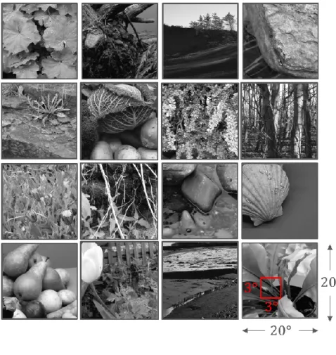
input, lateral geniculate nucleus (LGN) processing, and V1 activity (Figure 1B). To simulate 89
retinal activity corresponding to natural inputs, patches of size 3° × 3° (visual angles) were 90
sampled randomly from the Hunter-Hibbard database (Hunter & Hibbard, 2015) of natural 91
scenes (Figure 1A). 105 patches were used to train models corresponding to three encoding 92
schemes: ICA, SC and STDP. Each model used a specific procedure for implementing the LGN 93
processing and learning the synaptic weights between the LGN and V1 (see Figure 1B and 94
Methods).
96
Figure 1: Dataset and the computational pipeline. A. Training data. The Hunter-Hibbard dataset of natural images 97
was used. The images in the database have a 20° × 20° field of view. Patches of size 3° × 3° were sampled from 98
random locations in the images (overlap allowed). The same set of 100,000 randomly sampled patches was used 99
to train three models: Spike-timing dependent plasticity (STDP), Independent component analysis (ICA) and 100
Sparse coding (SC). B. Modelling the early visual pathway. Three representative stages of early visual computation 101
were captured by the models: retinal input, processing in the lateral geniculate nucleus (LGN), and the activity of 102
early cortical populations in the primary visual cortex (V1). Each input patch represented a retinal input. This was 103
followed by filtering operations generally associated with the LGN, such as decorrelation and whitening. Finally, 104
the output from the LGN units/filters was connected to the V1 population through all-to-all (dense) plastic synapses 105
which changed their weights during learning. Each model had a specific optimisation strategy for learning: the 106
STDP model relied on a local rank-based Hebbian rule, ICA minimised mutual information (approximated by the 107
negentropy), and SC enforced sparsity constraints on V1 activity. Abbreviations: DoG: Difference of Gaussian, 108
PCA: Principal component analysis. 109
110
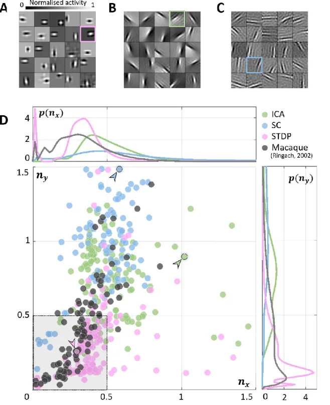
As expected, units in all models converged to oriented, edge-detector like RFs. While the RFs 111
from ICA (Figure 2B) and SC (Figure 2C) were elongated and highly directional, STDP (Figure 112
2A) RFs were more compact and less sharply tuned. This is in agreement with simple-cell 113
recordings in the macaque and cat, where studies have reported that not all RFs are optimally 114
tuned for edge-detection (Jones & Palmer, 1987; Ringach, 2002). A quantitative measure of 115
this phenomenon was obtained by fitting Gabor functions to the RFs and considering the 116
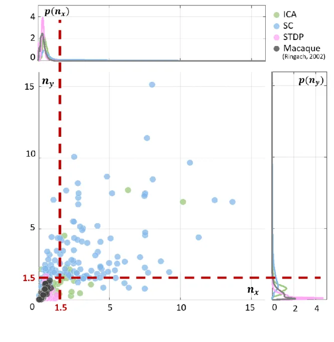
frequency-normalised spread vectors or FSVs (Ringach, 2002) of the fit. The first component 117
(𝑛𝑥) of the FSV characterises the number of lobes in the RF, and the second component (𝑛𝑦) is 118
a measure of the elongation of the RF (perpendicular to carrier propagation). A considerable 119
number of simple-cell RFs measured in macaque and cat tend to fall within the square bounded 120
by 𝑛𝑥 = 0.5 and 𝑛𝑦 = 0.5. The FSVs of a sample of neurones (𝑁 = 93) measured in the 121
macaque V1 (Ringach, 2002) indicate that 59.1% of the neurones lay within this region (Figure 122
2D). Since they are not elongated, and contain few lobes (typically 2-3 on/off regions), they 123
tend to be compact – making them less effective as edge-detectors compared to more crisply 124
tuned, elongated RFs. While a considerable number of STDP units (82.2%) tend to fall in this 125
realistic regime, ICA (10.7%) and SC (4.0%) show a distinctive shift upwards and to the right. 126
127
Figure 2: Receptive field (RF) shape. A, B, C. RFs of neurones randomly chosen from the three converged 128
populations. The STDP population is shown in A, ICA in B, and SC in C. D. Frequency-scaled spread vectors 129
(FSVs). FSV is a compact metric for quantifying RF shape. 𝑛𝑥 is proportional to the number of lobes in the RF, 130
𝑛𝑦 is a measure of the elongation of the RF, and values near zero characterise symmetric, often blobby RFs. The 131
FSVs for STDP (pink), ICA (green) and SC (blue), are shown with data from macaque V1 (black) (Ringach, 2002). 132
Measurements in macaque and cat simple-cells tend to fall within the square bound by 0.5 along both axes (shaded 133
in grey, with a dotted outline). Three representative neurones are indicated by colour-coded arrows: one for each 134
algorithm. The corresponding RFs are outlined in A, B and C using the corresponding colour. The STDP neurone 135
has been chosen to illustrate a blobby RF, the ICA neurone shows a multi-lobed RF, and the SC neurone illustrates 136
an elongated RF. Insets above and below the scatter plot show estimations of the probability density function for 137
𝑛𝑥 and 𝑛𝑦. Both axes have been cut-off at 1.5 to make comparison with biological data easier (complete 138
distributions are shown in Supplementary Figure S 1). 139
140
The inlays in Figure 2D provide estimations of the probability densities of two FSV parameters 141
for the macaque data and the three models. An interesting insight into these distributions is 142
given by the Kullback-Leibler (KL) divergence from the model distributions to the distribution 143
of the macaque data. KL divergence is a directed measure which can intuitively be interpreted 144
as the additional number of bits required if one of the three models were used to encode data 145
sampled from the macaque distribution. The KL divergence for the STDP model was found to 146
be 3.0 bits indicating that, on average, it would require three extra bits to encode data sampled 147
from the macaque distribution. In comparison, SC and ICA were found to require 8.4 and 14.6 148
additional bits respectively. An examination of the KL divergence of marginal distributions of 149
the FSV parameters (Supplementary Table S 1) suggests that STDP offers a better encoding of 150
both the 𝑛𝑥 (number of lobes) and the 𝑛𝑦 (compactness) parameters. 151
152
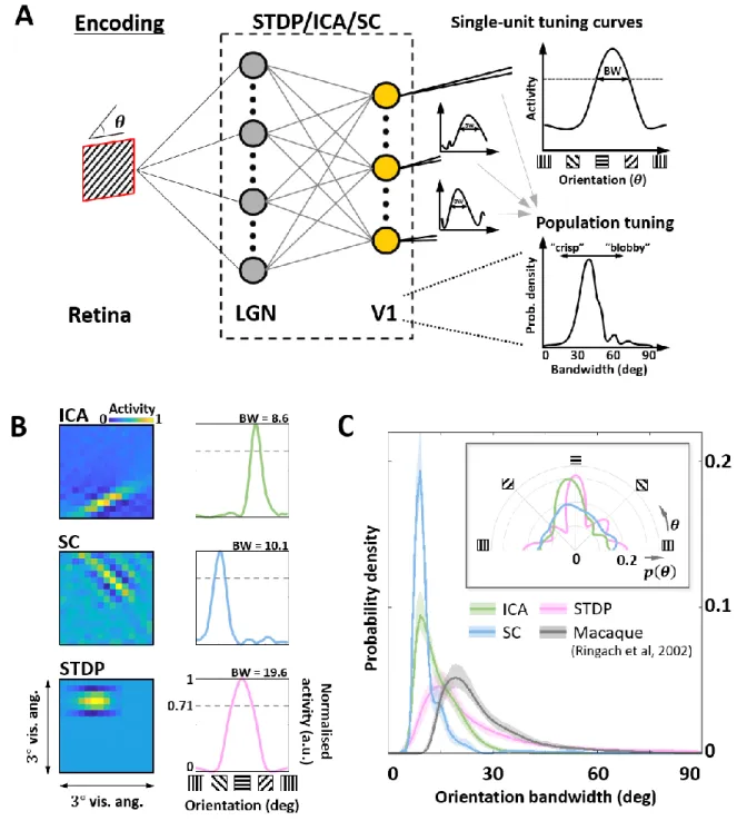
Given this sub-optimal, compact nature of STDP RF shapes, we next investigated how this 153
affected the responses of these neurones to sharp edges. In particular, we were interested in how 154
the orientation tuning curves of the units from the three models would compare to biological 155
data. We simulated a typical electrophysiological experiment to probe orientation tuning 156
(Figure 3A). To each unit, we presented noisy sine-wave gratings (SWGs) at its preferred 157
frequency and recorded its activity as a function of the stimulus orientation. This allowed us to 158
plot its orientation tuning curve (OTCs) (Figure 3B) and estimate the peak and tuning 159
bandwidth. While the peak indicates the preferred orientation of the unit, the bandwidth is a 160
measure of the local selectivity of the unit around its peak – low values corresponding to sharply 161
tuned neurones and higher values corresponding to broadly tuned, less selective neurones. For 162
all three models, we estimated the probability density functions of the OTC bandwidth, and 163
compared it to the distribution estimated over a large set of data (𝑁 = 308) measured in 164
macaque V1 (Ringach et al., 2002) (Figure 3C). The ICA and SC distributions peak at about 165
10-degrees (ICA: 9.1deg, SC: 8.5deg) while the STDP and macaque data have much broader 166
tunings (STDP: 15.1deg, Macaque data: 19.1deg). This is also reflected in the KL divergence 167
measured from the three model distributions to the macaque distribution (ICA: 2.4 bits, SC: 3.5 168
bits, STDP: 0.29 bits). 169
170
Figure 3: Orientation encoding. A. Orientation tuning. Sine-wave gratings with additive Gaussian noise (0dB SNR) 171
were presented to the three models to obtain single-unit orientation tuning curves (OTCs). OTC peak identifies the 172
preferred orientation of the unit, and OTC bandwidth (half width at 1/√2 peak response) is a measure of its 173
selectivity around the peak. Low bandwidth values are indicative of sharply tuned units while high values signal 174
broader, less specific tuning. B. Single-unit tuning curves. RF (left) and the corresponding OTC (right) for 175
representative units from ICA (top row, green), SC (second row, blue) and STDP (bottom row, pink). The 176
bandwidth is shown above the OTC. C. Population tuning. Estimated probability density of the OTC bandwidth 177
for the three models (same colour code as panel B), and data measured in macaque V1 (black) (Ringach et al., 178
2002). The inlay shows estimated probability density of the preferred orientation for the three models. 179
180
After characterising the encoding capacity of the models, we next probed the possible 181
downstream implications of such codes. The biological goal of most neural code, in the end, is 182
the generation of behaviour that maximises evolutionary fitness. However, due to the 183
complicated neural apparatus that separates behaviour from early sensory processing, it is not 184
straightforward (or at times, even possible) to analyse the interaction between the two. Here, 185
we make use of two separate metrics to investigate this relationship. In both cases, the models 186
were presented with oriented SWGs, followed by an analysis of the resulting population activity 187
(Figure 4A). 188
189
In the first analysis, we estimated the Fisher information (FI) contained in the generated 190
responses. Orientation discrimination tasks are particularly suited to such an analysis (i.e., the 191
study of a behavioural measure using early sensory activity) as V1 activity has been shown to 192
correlate with orientation discrimination thresholds (Vogels & Orban, 1990), something that 193
has not been observed for other visual properties such as binocular disparity (Nienborg & 194
Cumming, 2006) or motion (Grunewald et al., 2002). Given the responses of an encoding 195
model, the Crámer-Rao bound permits us to use the FI to draw inferences about the optimal 196
discrimination performance – leading to the simulation of what could be called a locally-197
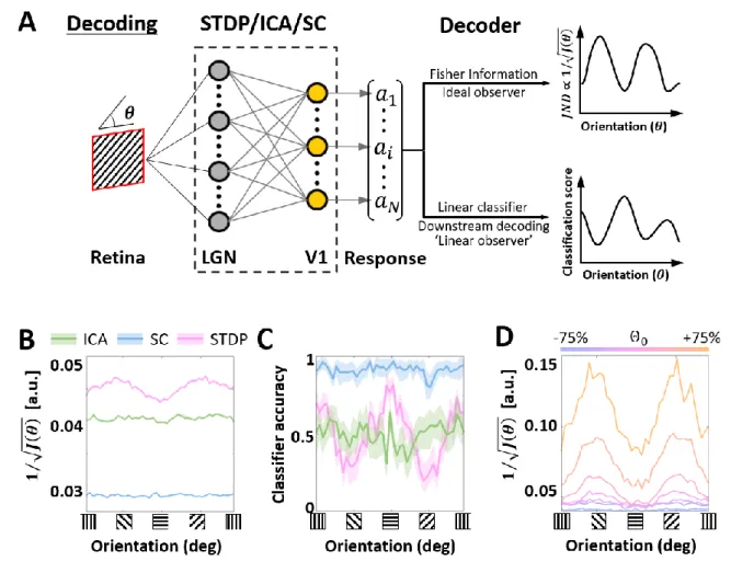
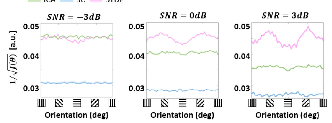
optimal ideal observer (Wei & Stocker, 2017). We find that ICA and SC ideal observers have 198
lower thresholds (i.e., a better orientation discrimination performance) compared to STDP 199
(Figure 4B). Considering the sharper population tuning of the ICA and SC models, this is not 200
surprising. Interestingly, the STDP ideal observer shows a bias for cardinal orientations 201
(horizontal and vertical gratings), while ICA and SC ideal observers show uniform performance 202
across all stimulus orientations. 203
204
Figure 4: Orientation decoding. A. Retrieving encoded information. Sine-wave gratings (SWGs) with additive 205
Gaussian noise at 0dB were presented to the three models. The following question was then posed: how much 206
information about the stimulus (in this case, the orientation) can be decoded from the population responses? The 207
theoretical limit of the accuracy of such a decoder can be approximated by estimating the Fisher information (FI) 208
in the responses. This can be interpreted as the response of an ideal observer capable of extracting all the 209
information contained in the population responses. In addition, a linear decoder was also used to directly decode 210
the population responses. This could be a downstream process which is linearly driven by the population activity, 211
or a less-than-optimal ‘linear observer’. B. Ideal observer (Fisher information). The abscissa shows the stimulus 212
orientation, and the ordinate shows the inverse square-root of the estimated FI. Due to the Cramér-Rao bound, low 213
values on the ordinate denote more precise encoding of the orientation, while higher values denote lower precision. 214
Results for ICA are shown in green, SC in blue, and STDP in pink. C. Linear decoding. The stimuli and responses 215
from B were used to train a linear-discriminant classifier. The ordinate shows the accuracy (probability of correct 216
classification) for each ground-truth value of the stimulus orientation (abscissa). The same symbols as B are used, 217
and envelopes around the solid lines show 95% confidence intervals. D. Post-training threshold variation in STDP. 218
The SWG stimuli used in C were used to test STDP models with different values of the threshold parameter, which 219
represents the threshold potential of the neurones in the model. The threshold was either increased (by 25%, 50% 220
or 75%) or decreased (by 25%, 50% or 75%) with respect to the training threshold (denoted by Θ0). The abscissa 221
and ordinate denote the same quantities as B, and each line shows the ideal observer response from one of the 222
models. The magnitude of change in the threshold is denoted by a corresponding change in colour from pink (Θ0) 223
to orange (increase) or blue (decrease). 224
225
Although the FI ideal observer represents the optimal decoding of a given encoding scheme, it 226
does not automatically follow that all the encoded information is available for downstream 227
processing (Quiroga & Panzeri, 2009). This is especially true in the presence of significant 228
higher-order correlations (Shamir & Sompolinsky, 2004). To investigate more realistic 229
orientation decoding in the three models, we implemented a second analysis where we reduced 230
the complexity of the decoding and examined the performance of a decoder built on linear 231
discriminant classifiers (these classifiers assume fixed first-order correlations in the input). 232
Such decoders could be interpreted as linearly-driven feedforward populations downstream 233
from the thalamo-recipient layer (the ‘V1’ populations in the three models), or a simplified, 234
‘linear’ observer. In general, we found the decoding performance (Figure 4C) to be consistent 235
with ideal observer predictions (Figure 4B), indicating that linear correlations represent a 236
sizeable amount of correlations in all three encoding schemes. Both ICA and SC showed 237
uniform decoding scores across the orientations, with SC being the most accurate of the three 238
models. Once again, STDP showed a modulation at the cardinal orientations, with the scores 239
being almost three times higher at the peaks (horizontal and vertical gratings) than the troughs. 240
241
Since the STDP model is linear up to a thresholding operation, we hypothesised that the 242
modulation in decoding (Figure 4A and B) must result from the intervening thresholding 243
nonlinearity. To test this hypothesis, we ran simulations where the threshold parameter 244
(analogue of the threshold potential in the STDP model) was either increased or decreased. 245
Note that in all simulations the model was first trained (i.e., synaptic learning using natural 246
stimuli, see Figure 1) using the same ‘training’ threshold, and the increase/decrease of the 247
threshold parameter was imposed post-convergence. Our results (Figure 4D) showed that the 248
modulation of the classification performance for horizontal and vertical gratings became more 249
pronounced as the threshold was increased, and flattened as the threshold was decreased. 250
However, this increase in the cardinal orientation bias came at the cost of an overall decrease 251 in precision. 252 253 Discussion 254
Traditionally, process-based descriptions (often studied through mean-field statistics under 255
large N limits) have been used to model fine-grained neuronal dynamics (Harnack et al., 2015; 256
Kang & Sompolinsky, 2001; Moreno-Bote et al., 2014), while more global, normative schemes 257
are employed to predict population-level characteristics (Hoyer & Hyvärinen, 2000; Lee & 258
Seung, 1999; Olshausen & Field, 1997; van Hateren & van der Schaaf, 1998). Detailed process-259
based models suffer from constraints imposed by computational complexity, prohibitively long 260
execution times (which do not scale well for large networks), and hardware that is geared 261
towards synchronous processing. On the other hand, most one-shot models can leverage faster 262
computational libraries and architectures developed over decades, thereby leading to more 263
efficient and scalable computation. Through this work, we argue that more abstract forms of 264
process-based models, when used to answer specific questions, can still give a closer 265
approximation of biological processes than normative schemes. Our model, despite important 266
limitations such as the use of at most one spike per neuron, lack of cortico-cortical connections, 267
and feedback from higher visual areas, is still able to describe a number of phenomena which 268
are not predicted by normative schemes. 269
The converged RFs of the STDP model are closer to those reported in electrophysiological 271
measurements in the macaque. A number of them display a characteristic departure from the 272
optimal, sharply tuned edge-detectors predicted by ICA and SC (Figure 2). This suboptimal 273
shape also results in suboptimal orientation encoding, which, once again, was found to be closer 274
to data measured in the macaque V1 (Figure 3). Furthermore, decoding from this population 275
shows a distinct bias for horizontal and vertical stimuli, with the performance for the cardinal 276
orientations being roughly two times better than other orientations (Figure 4). Interestingly, this 277
bias for cardinal directions has also been observed in human participants (Orban et al., 1984), 278
who also show an almost two-fold reduction in just-noticeable-differences for horizontal and 279
vertical stimuli (Heeley & Timney, 1988). Our results suggest that such behavioural biases for 280
cardinal directions (the so-called oblique effect) are supported by the cortical architecture as 281
early as the early thalamocortical interface – a claim that is further reinforced by 282
electrophysiology (Dragoi et al., 2001; Li et al., 2003) and imaging experiments (Furmanski & 283
Engel, 2000) which suggest that neural activity in the primary visual cortex may be directly 284
correlated with the perceptual oblique effect. 285
286
Moreover, our simulations also demonstrated that the magnitude of the cardinal orientation bias 287
in the STDP model can be changed by manipulating the spiking threshold (Figure 4D). Thus, 288
even after the initial learning phase has ended, the network is still theoretically capable of 289
shrinking or expanding its encoded dictionary without modifying its synaptic connectivity – 290
simply by modulating its threshold. In the cortex, such changes are likely to be mediated by 291
homeostatic processes (Harnack et al., 2015; Perrinet, 2019) and metaplastic regulation 292
(Abraham, 2008; Cooke & Bear, 2010). This supports the idea that purely bottom-up changes 293
are indeed capable of driving perceptually relevant cortical changes in adults who are beyond 294
the critical window of plasticity – an observation of particularly relevance for reports claiming 295
that low-level changes in the early visual cortex may accompany perceptual learning (Bao et 296
al., 2010; Furmanski et al., 2004). In the context of the current model, this is only possible if 297
the information content in the non-spiking activity is larger than the spiking activity (Figure S 298
5), and suggests that the model may employ some form of variable-length encoding. This 299
becomes especially pertinent for realistic natural inputs which are more complicated and varied 300
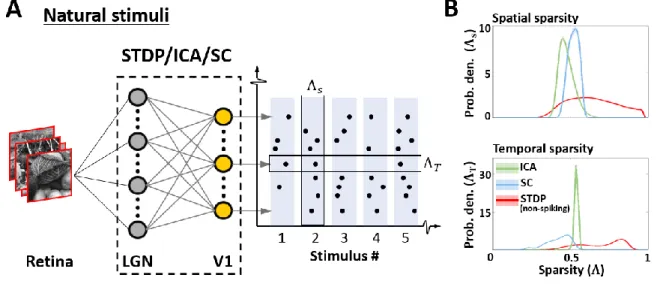
than SWGs. When we characterised the sparsity of non-spiking activity for each of the three 301
models using naturalistic stimuli (Figure 5A), our results (Figure 5B) confirmed that the STDP 302
responses do indeed show a higher variability in sparsity when measured across both the 303
encoding ensemble (‘spatial sparsity’), and the input sequence (‘temporal sparsity’). Thus, the 304
sparsity of the STDP neurones is stimulus-dependent, and likely driven by the relative 305
probability of occurrence of specific features in the dataset. 306
307
308
Figure 5: Sparsity of responses to natural stimuli. A. Sparsity indices. To estimate the sparsity of the non-spiking 309
responses to natural stimuli, 104 patches (3° × 3° visual angle) randomly sampled from natural scenes were 310
presented to the three models. Two measures of sparsity were defined: Spatial sparsity Index (Λ𝑆) was defined as 311
the average sparsity of the activity of the entire neuronal ensemble, while Temporal sparsity Index (Λ𝑇) was 312
defined as the average sparsity of the activity of single neurones to the entire input sequence. B. Spatial and 313
temporal sparsity. The top panel shows the estimated probability density of Λ𝑆 for ICA (green), Sparse coding 314
(blue) and STDP (red). Λ𝑆 varied between 0 (all units activate with equal intensity) and 1 (only one unit activates) 315
by definition. The bottom panel shows the estimated probability density of Λ𝑇 in a manner analogous to Λ𝑆. Λ𝑇 316
also varied between 0 (homogeneous activity for the entire input sequence) and 1 (activity only for few inputs in 317
the sequence). 318
319
The encoding that emerges from localised learning, as we have shown, can confer biological 320
advantages while being sub-optimal in a global information-theoretic framework. This 321
dichotomy has indeed been characterised at various stages of the early visual system (Chelaru 322
& Dragoi, 2008; Field & Chichilnisky, 2007; Liu et al., 2009; Ringach, 2002; Ringach et al., 323
2002), and offers an interesting glimpse into the notion of ‘optimality’ in biological systems. In 324
such systems input information is not the only criterion of fitness, and the landscape is 325
modulated by factors such as the topological and dynamical constraints of the learning 326
mechanisms, decoding capabilities of the downstream apparatus, and relevance of the resulting 327
behaviour(s) to the functioning and survival of the organism. Given these realistic and 328
complicated constraints, it is obvious that a clear global optimisation function which describes 329
the responses of real neural populations is very difficult, if not impossible, to formulate. This 330
makes an ideal case for the use of process-based, local descriptions which, by definition, offer 331
a much deeper insight into the organisation and functioning of biological systems. Such models 332
offer the flexibility to not only describe normative hypotheses about stimulus encoding, but to 333
also predict how meaningful internal parameters and interactions in the model impact the 334
behaviour of the system. With increasingly common availability of faster and more adaptable 335
computing solutions, we hope process-based modelling will be adopted more widely by 336
cognitive and computational neuroscientists. 337
338
Finally, it must be noted that in this study we have used classical forms of the ICA and SC 339
algorithms. More generally, these models are part of a class of data-adaptive encoding schemes 340
which also comprises other algorithms such as principal-component analysis (PCA) and 341
nonnegative matrix factorisation (NMF). These algorithms rely on the optimality of the 342
encoding manifold at representing the training data, and their use in neuroscience is motivated 343
by the proven energetic and information-theoretic efficiency of neural processes at representing 344
natural statistics. We would like to draw attention to a growing number of insightful studies 345
based on hybrid encoding schemes which address multiple optimisation criteria (Beyeler et al., 346
2019; Martinez-Garcia et al., 2017; Perrinet & Bednar, 2015), often through local process-based 347
computation (Isomura & Toyoizumi, 2018; Savin et al., 2010; Zylberberg et al., 2011). 348
Methods 350
Dataset 351
The Hunter-Hibbard dataset of natural images was used (Hunter & Hibbard, 2015). It is 352
available under the MIT license at https://github.com/DavidWilliamHunter/Bivis, and consists 353
of 139 stereoscopic images of natural scenes captured using a realistic acquisition geometry 354
and a 20 degree field of view. Only images from the left channel were used, and each image 355
was resized to a resolution of 5 pixels/degree along both horizontal and vertical directions. 356
Inputs to all encoding schemes were 3 × 3 degree patches (i.e. 15 × 15 pixels) sampled 357
randomly from the dataset (Figure 1A). 358
359
Encoding models 360
Samples from the dataset were used to train and test three models corresponding to ICA, SC 361
and STDP encoding schemes. Each model consisted of three successive stages (Figure 1B). The 362
first stage represented retinal activations. This was followed by a pre-processing stage 363
implementing operations which are typically associated with processing in the LGN, such as 364
whitening and decorrelation. In the third stage, LGN output was used to drive a representative 365
V1 layer. 366
367
During learning, 105 patches (3 × 3 degree) were randomly sampled from the dataset to 368
simulate input from naturalistic scenes. In this phase, the connections between the LGN and V1 369
layers were plastic, and modified in accordance with one of the three encoding schemes. Care 370
was taken to ensure that the sequence of inputs during learning was the same for all three 371
models. After training, the weights between the LGN and V1 layers were no longer allowed to 372
change. The implementation details of the three models are described below. 373
374
Sparse Coding
375
SC algorithms are based on energy-minimisation, which is typically achieved by a 376
‘sparsification’ of activity in the encoding population. We used a now-classical SC scheme 377
proposed by (Olshausen & Field, 1996, 1997). The pre-processing in this algorithm consists of 378
an initial whitening of the input using low pass filtering, followed by a trimming of higher 379
frequencies. The latter was employed to counter artefacts introduced by high frequency noise, 380
and the effects of sampling across a uniform square grid. In the frequency domain the pre-381
processing filter was given by a zero-phase kernel: 382 𝐻(𝑓) = 𝑓 ⋅ 𝑒−( 𝑓 𝑓0) 4 383
Here, 𝑓0 = 10 cycles/degree is the cut-off frequency. The outputs of these LGN filters were 384
then used as inputs to the V1 layer composed of 225 units (3° × 3° RF at 5 pixels/degree). 385
Retinal projections of the converged RFs (Figure 2C) were recovered by an approximate 386
reverse-correlation algorithm (Ringach, 2002; Ringach & Shapley, 2004) derived from a linear-387
stability analysis of the SC objective function about its operating point. The RFs (denoted as 388
columns of a matrix, say 𝝃) were given by: 389
𝝃 = 𝑨[𝑨𝑇𝑨 + 𝜆𝑆"(0)𝑰]−1 390
Here, 𝑨 is the matrix containing converged sparse components as column vectors, 𝜆 is the 391
regularisation parameter (for the reconstruction, it is set to 0.14𝜎, where 𝜎2 is the variance in 392
the input dataset), and 𝑆(𝑥) is the shape-function for the prior distribution of the sparse 393
coefficients (this implementation uses 𝑙𝑜𝑔 (1 + 𝑥2)). 394
Independent Component Analysis (ICA)
396
ICA algorithms are based on the idea that the activity of an encoding ensemble must be as 397
information-rich as possible. This typically involves a maximisation of mutual information 398
between the retinal input and the activity of the encoding ensemble. We used a classical ICA 399
algorithm called fastICA (Hyvärinen & Oja, 2000) which achieves this through an iterative 400
estimation of input negentropy. The pre-processing in this implementation was performed using 401
a truncated Principal Component Analysis (PCA) transform (𝑑̃ = 150 components were used), 402
leading to low-pass filtering and local decorrelation akin to centre-surround processing reported 403
in the LGN. If the input patches are denoted by the columns of a matrix (say 𝑿), the LGN 404
activity 𝑳 can be written as: 405
𝑳 = 𝑼̃𝑇𝑿 𝐶 406
Here, 𝑿𝐶 = 𝑿 − 〈𝑿〉 and 𝑼̃ is a matrix composed of the first 𝑑̃ (= 150) principal components 407
of 𝑿𝐶. The activity of these LGN filters was then used to drive the ICA V1 layer consisting of 408
150 units, with its activity 𝚺 being given by: 409
𝜮 = 𝑾𝑳 410
Here, 𝑾 is the un-mixing matrix which is optimised during learning. The recovery of the RFs 411
for ICA was relatively straight forward, as, in our implementation, they were assumed to be 412
equivalent to the filters which must be applied to a given input to generate the corresponding 413
V1 activity. The RFs (denoted as columns of a matrix, say 𝝃) were given by: 414
𝝃 = 𝑼̃𝑾𝑇+ 〈𝑿〉 415
Spike timing dependent plasticity (STDP)
417
STDP is a biologically observed, Hebbian-like learning rule which relies on local 418
spatiotemporal patterns in the input. We used a feedforward model based on an abstract rank-419
based STDP rule (Chauhan et al., 2018). The pre-processing in the model consisted of ON/OFF 420
filtering using difference-of-Gaussian filters based on the properties of magno-cellular LGN 421
cells. The outputs of these filters were converted to relative first-spike latencies using a 422
monotonically decreasing function (1/𝑥 was used), and only the earliest 10% spikes were 423
allowed to propagate to V1 (Delorme et al., 2001; Masquelier & Thorpe, 2007). These spikes 424
were used to drive an unsupervised network of 225 (non-leaky) integrate-and-fire neurones. 425
During learning, changes in the synaptic weights between LGN and V1 were governed by a 426
simplified version of the STDP rule proposed by (Gütig et al., 2003). After each iteration, the 427
change (Δ𝑤) in the weight (𝑤) of a given synapse was given by: 428
Δ𝑤 = { −𝛼
−⋅ 𝑤𝜇−, Δ𝑡 ≤ 0 𝛼+⋅ (1 − 𝑤)𝜇+, Δ𝑡 > 0 429
Here, 𝛥𝑡 is the difference between the post- and pre-synaptic spike times, and the constants 𝛼± 430
and 𝜇± describe the learning-rate and non-linearity of the process respectively. Thus, the weight 431
was increased if a presynaptic spike occurred before the postsynaptic spike (causal firing), and 432
decreased if it occurred after the post-synaptic spike (acausal firing). During each iteration of 433
learning, the population followed a winner-take-all inhibition rule wherein the firing of one 434
neurone reset the membrane potentials of all other neurones. After learning, this inhibition was 435
no longer active and multiple units were allowed to fire for each input. The RFs of the 436
converged neurones were recovered using a linear approximation. If 𝑤𝑖 denotes the weight of 437
the synapse connecting a given neurone to the 𝑖th LGN filter, the RF 𝝃 of the neurone was given 438
by: 439
𝝃 = ∑ 𝑤𝑖𝝍𝑖 𝑖∈𝐿𝐺𝑁 440
Here, 𝝍𝑖 is the RF of the 𝑖th LGN neurone. 441 442 Evaluation metrics 443 Gabor fitting 444
Linear approximations of RFs (Figure 2, panels A, B and C) obtained by each encoding strategy 445
were fitted using 2-D Gabor functions. This is motivated by the fact that all the encoding 446
schemes considered here lead to linear, simple-cell-like RFs. In this case, the goodness-of-fit 447
parameter (𝑅2) provides an intuitive measure of how Gabor-like a given RF is. The fitting was 448
carried out using an adapted version of the code available here, generously shared under an 449
open-source license by Gerrit Ecke (University of Tübingen). 450
451
Frequency-normalised spread vector
452
The shape of the RFs approximated by each encoding strategy was characterised using 453
frequency-normalised spread vectors (FSVs) (Chauhan et al., 2018; Ringach, 2002). For a RF 454
fitted by a Gabor-function with sinusoid carrier frequency 𝑓 and envelope size 𝜎 = [𝜎𝑥 𝜎𝑦]𝑇, 455
the FSV is given by: 456
[𝑛𝑥 𝑛𝑦]𝑇 = [𝜎𝑥 𝜎𝑦]𝑇𝑓 457
While 𝑛𝑥 provides an intuition of the number of cycles in the RF, 𝑛𝑦 is a cycle-adjusted measure 458
of the elongation of the RF perpendicular to the direction of sinusoid propagation. The FSV 459
serves as a compact, intuitive descriptor of the RF shape-invariance to affine operations such 460
as translation, rotation and isotropic scaling. 461
462
Fisher Information
463
The information content in the activity of the converged units was quantified by using 464
approximations of the Fisher information (FI, denoted here by the symbol Φ). If 𝒙 = 465
{𝑥1, 𝑥2, 𝑥3, … , 𝑥𝑁} is a random variable describing the activity of an ensemble of 𝑁 independent 466
units, the FI of the population with respect to a parameter 𝜃 is given by: 467 Φ(𝜃) = ∑ 𝐸 [{𝜕 𝑙𝑛 𝑙𝑛 𝑃(𝑥𝑖|𝜃) 𝜕𝜃 } 2 ] 𝑃(𝑥𝑖|𝜃) 𝑁 𝑖=1 468
Here, 𝐸[. ]𝑃(𝑥𝑖|𝜃) denotes expectation value with respect to the firing-state probabilities of the 469
𝑖𝑡ℎ neurone in response to the stimuli corresponding to parameter value 𝜃. In our simulations, 470
𝜃 was the orientation (defined as the direction of travel) of a set of sine-wave gratings (SWGs) 471
with additive Gaussian noise. The SWGs were presented at frequency of 1.25cycles/visual 472
degree, and the responses were calculated by averaging over 8 evenly spaced phase values in 473
[0°, 360°). This effectively simulated a drifting grating design within the constraints of the 474
computational models. In Figure 4 (panels B and D) we report values for an SNR of 0dB (i.e., 475
the signal and noise had equal variance – a fairly noisy condition), but the behaviour of the 476
system was found to be similar for SNR values of -3dB and 3dB (Supplementary Figure S 2). 477
The ground-truth values of 𝜃 were sampled at intervals of 4° in the range [0°, 180°), and each 478
simulation was repeated 100 times. 479
Decoding using a linear classifier
481
In addition to FI approximations, we also used a linear decoder on the population responses 482
obtained in the FI analysis. The decoder was an error-correcting output codes model composed 483
of binary linear-discriminant classifiers configured in a one-vs.-all scheme. Similar to the FI 484
experiment, ground-truth values of the orientation at intervals of 4° in the range [0°, 180°) were 485
used as the class labels, and the activity generated by the corresponding SWG stimuli with 486
added Gaussian noise was used as the training/testing data. The SWGs were presented at 487
frequency of 1.25cycles/visual degree, and the responses were calculated by averaging over 8 488
evenly spaced phase values in [0°, 360°). Each simulation was repeated 100 times, each time 489
with 5-fold validation. Figure 4C shows the results for a 0dB SNR, but the overall trends 490
remained unchanged for -3dB and 3dB SNR levels (Supplementary Figure S 3). 491
492
Post-convergence threshold variation in STDP
493
To test how post-learning changes in the threshold affect the specificity of a converged network, 494
we tested an STDP network trained using a threshold 𝛩𝑡𝑟𝑎𝑖𝑛𝑖𝑛𝑔 by increasing or decreasing its 495
threshold (to say, 𝛩𝑡𝑒𝑠𝑡𝑖𝑛𝑔) and presenting it with SWGs (same stimuli as the ones used to 496
calculate the FI). We report the results of seven simulations where the relative change in 497
threshold was given by 25% increments/decrements, i.e.: 498
𝛩𝑡𝑒𝑠𝑡𝑖𝑛𝑔− 𝛩𝑡𝑟𝑎𝑖𝑛𝑖𝑛𝑔
𝛩𝑡𝑟𝑎𝑖𝑛𝑖𝑛𝑔 = {0, ±0.25, ±0.50, ±0.75} 499
The results reported in Figure 4D were calculated for an input SNR of 0dB, but similar results 500
were obtained for -3 and 3dB SNR as well (Supplementary Figure S 4). 501
Kullback-Leibler divergence
503
For each model, we estimated probability density functions (pdfs) over parameters such as the 504
FSVs and the population bandwidth. To quantify how close the model pdfs were to those 505
estimated from the macaque data, we employed the Kullback-Leibler (KL) divergence. KL 506
divergence is a directional measure of distance between two probability distributions. Given 507
two distributions 𝑃 and 𝑄 with corresponding probability densities 𝑝 and 𝑞, the KL divergence 508
(denoted 𝐷𝐾𝐿) from a 𝑄 to 𝑃 is given by: 509
𝐷𝐾𝐿(𝑃||𝑄) = ∫ 𝑝(𝒙) log2(𝑝(𝒙) 𝑞(𝒙)) 𝑑𝒙 𝛀
510
Here, 𝛀 is the support of the distribution 𝑄. In our analysis, we considered 𝑝 as a pdf estimated 511
from the macaque data, and 𝑞 as the pdf (of the same variable) estimated using ICA, SC or 512
STDP. In this case, KL divergence lends itself to a very intuitive interpretation: it can be 513
considered as the additional bandwidth (in bits) which would be required if the biological 514
variable were to be encoded using one of the three computational models. Note that 𝑃 and 𝑄 515
may be multivariate distributions. 516
517
Sparsity: Gini index
518
The sparseness of the encoding was evaluated using the Gini index (GI). GI is a measure which 519
characterises the deviation of the population-response from a uniform distribution of activity 520
across the samples. It is 0 if all units have the same response and tends to 1 as the responses 521
become sparser (being equal to 1 if only one unit responds, while others are silent). It is invariant 522
to the range of the responses within a given sample, and robust to variations in sample-size 523
(Hurley & Rickard, 2009). Formally, the GI (denoted here as Λ) is given by: 524
Λ(𝒙) = 1 − 2 ∫ 𝐿(𝐹) 1 0
𝑑𝐹 525
Here, 𝐿 is the Lorenz function defined on the cumulative probability distribution 𝐹 of the neural 526
activity (say, 𝒙). We defined two variants of the GI which measure the spatial (Λs) and temporal 527
sparsity (Λt) of an ensemble of encoders (Figure 5A). Given a sequence of 𝑀 inputs to an 528
ensemble of 𝑁 neurones, the spatial sparsity of the ensemble response to the 𝑚th stimulus is 529 given by: 530 ΛS(𝑚) = Λ( {𝑥𝑚1 , 𝑥 𝑚2, … , 𝑥𝑚𝑁} ) 531
Here, 𝑥𝑚𝑛 denotes the activity of the 𝑛th neurone in response to the 𝑚th input. Similarly, the 532
temporal sparsity of the 𝑛th neurone over the entire sequence of inputs is given by: 533 ΛT(𝑛) = Λ( {𝑥1𝑛, 𝑥 2𝑛, … , 𝑥𝑀𝑛} ) 534 535 Code 536
The code for ICA was written in python using the sklearn library which implements the classical 537
fastICA algorithm. The code for SC was based on the C++ and Matlab code shared by Prof.
538
Bruno Olshaussen. The STDP code was based on a previously published binocular-STDP 539
algorithm available here. 540
Bibliography 542
Abraham, W. C. (2008). Metaplasticity: Tuning synapses and networks for plasticity. Nature 543
Reviews Neuroscience, 9(5), 387. https://doi.org/10.1038/nrn2356
544
Anderson, C., Van Essen, D., & Olshausen, B. (2005). CHAPTER 3—Directed Visual 545
Attention and the Dynamic Control of Information Flow. In L. Itti, G. Rees, & J. K. 546
Tsotsos (Eds.), Neurobiology of Attention (pp. 11–17). Academic Press. 547
https://doi.org/10.1016/B978-012375731-9/50007-0 548
Bao, M., Yang, L., Rios, C., He, B., & Engel, S. (2010). Perceptual learning increases the 549
strength of the earliest signals in visual cortex. The Journal of Neuroscience : The 550
Official Journal of the Society for Neuroscience, 30(45), 15080–15084.
551
https://doi.org/10.1523/JNEUROSCI.5703-09.2010 552
Bell, A., & Sejnowski, T. (1997). The “independent components” of natural scenes are edge 553
filters. Vision Research, 37(23), 3327–3338. https://doi.org/10.1016/S0042-554
6989(97)00121-1 555
Beyeler, M., Rounds, E., Carlson, K., Dutt, N., & Krichmar, J. (2019). Neural correlates of 556
sparse coding and dimensionality reduction. PLOS Computational Biology, 15(6), 557
e1006908. https://doi.org/10.1371/journal.pcbi.1006908 558
Brito, C. S. N., & Gerstner, W. (2016). Nonlinear Hebbian Learning as a Unifying Principle in 559
Receptive Field Formation. PLOS Computational Biology, 12(9), e1005070. 560
https://doi.org/10.1371/journal.pcbi.1005070 561
Bruce, N., Rahman, S., & Carrier, D. (2016). Sparse coding in early visual representation: From 562
specific properties to general principles. Neurocomputing, 171, 1085–1098. 563
https://doi.org/10.1016/j.neucom.2015.07.070 564
Caporale, N., & Dan, Y. (2008). Spike Timing–Dependent Plasticity: A Hebbian Learning 565
Rule. Annual Review of Neuroscience, 31(1), 25–46. 566
https://doi.org/10.1146/annurev.neuro.31.060407.125639 567
Chauhan, T., Masquelier, T., Montlibert, A., & Cottereau, B. (2018). Emergence of binocular 568
disparity selectivity through Hebbian learning. The Journal of Neuroscience, 38(44), 569
9563–9578. https://doi.org/10.1523/JNEUROSCI.1259-18.2018 570
Chelaru, M. I., & Dragoi, V. (2008). Efficient coding in heterogeneous neuronal populations. 571
Proceedings of the National Academy of Sciences, 105(42), 16344–16349.
572
https://doi.org/10.1073/pnas.0807744105 573
Cooke, S., & Bear, M. (2010). Visual Experience Induces Long-Term Potentiation in the 574
Primary Visual Cortex. Journal of Neuroscience, 30(48), 16304–16313. 575
https://doi.org/10.1523/JNEUROSCI.4333-10.2010 576
Delorme, A., Perrinet, L., & Thorpe, S. J. (2001). Networks of integrate-and-fire neurons using 577
Rank Order Coding B: Spike timing dependent plasticity and emergence of orientation 578
selectivity. Neurocomputing, 38–40, 539–545. https://doi.org/10.1016/S0925-579
2312(01)00403-9 580
Dragoi, V., Turcu, C. M., & Sur, M. (2001). Stability of Cortical Responses and the Statistics 581
of Natural Scenes. Neuron, 32(6), 1181–1192. https://doi.org/10.1016/S0896-582
6273(01)00540-2 583
Field, G. D., & Chichilnisky, E. J. (2007). Information Processing in the Primate Retina: 584
Circuitry and Coding. Annual Review of Neuroscience, 30(1), 1–30. 585
https://doi.org/10.1146/annurev.neuro.30.051606.094252 586
Furmanski, C., & Engel, S. (2000). An oblique effect in human primary visual cortex. Nature 587
Neuroscience, 3(6), 535–536. https://doi.org/10.1038/75702
Furmanski, C., Schluppeck, D., & Engel, S. (2004). Learning Strengthens the Response of 589
Primary Visual Cortex to Simple Patterns. Current Biology, 14(7), 573–578. 590
https://doi.org/10.1016/j.cub.2004.03.032 591
Geisler, W. (2008). Visual perception and the statistical properties of natural scenes. Annual 592
Review of Psychology, 59, 167–192.
593
https://doi.org/10.1146/annurev.psych.58.110405.085632 594
Grunewald, A., Bradley, D., & Andersen, R. (2002). Neural Correlates of Structure-from-595
Motion Perception in Macaque V1 and MT. Journal of Neuroscience, 22(14), 6195– 596
6207. https://doi.org/10.1523/JNEUROSCI.22-14-06195.2002 597
Gütig, R., Aharonov, R., Rotter, S., & Sompolinsky, H. (2003). Learning Input Correlations 598
through Nonlinear Temporally Asymmetric Hebbian Plasticity. Journal of 599
Neuroscience, 23(9), 3697–3714.
600
Harnack, D., Pelko, M., Chaillet, A., Chitour, Y., & Rossum, M. C. W. van. (2015). Stability 601
of Neuronal Networks with Homeostatic Regulation. PLOS Computational Biology, 602
11(7), e1004357. https://doi.org/10.1371/journal.pcbi.1004357
603
Heeley, D., & Timney, B. (1988). Meridional anisotropies of orientation discrimination for sine 604
wave gratings. Vision Research, 28(2), 337–344. https://doi.org/10.1016/0042-605
6989(88)90162-9 606
Hoyer, P., & Hyvärinen, A. (2000). Independent component analysis applied to feature 607
extraction from colour and stereo images. Network: Computation in Neural Systems, 608
11(3), 191–210. https://doi.org/10.1088/0954-898X_11_3_302
609
Hübener, M., & Bonhoeffer, T. (2014). Neuronal Plasticity: Beyond the Critical Period. Cell, 610
159(4), 727–737. https://doi.org/10.1016/j.cell.2014.10.035
611
Hunter, D., & Hibbard, P. (2015). Distribution of independent components of binocular natural 612
images. Journal of Vision, 15(13), 6. https://doi.org/10.1167/15.13.6 613
Hurley, N., & Rickard, S. (2009). Comparing Measures of Sparsity. IEEE Transactions on 614
Information Theory, 55(10), 4723–4741. https://doi.org/10.1109/TIT.2009.2027527
615
Hyvärinen, A., & Oja, E. (2000). Independent component analysis: Algorithms and 616
applications. Neural Networks, 13(4–5), 411–430. https://doi.org/10.1016/S0893-617
6080(00)00026-5 618
Isomura, T., & Toyoizumi, T. (2018). Error-Gated Hebbian Rule: A Local Learning Rule for 619
Principal and Independent Component Analysis. Scientific Reports, 8(1), 1835. 620
https://doi.org/10.1038/s41598-018-20082-0 621
Jones, J., & Palmer, L. (1987). An evaluation of the two-dimensional Gabor filter model of 622
simple receptive fields in cat striate cortex. Journal of Neurophysiology, 58(6), 1233– 623
1258. 624
Larsen, R. S., Rao, D., Manis, P. B., & Philpot, B. D. (2010). STDP in the Developing Sensory 625
Neocortex. Frontiers in Synaptic Neuroscience, 2, 9. 626
https://doi.org/10.3389/fnsyn.2010.00009 627
Lee, D., & Seung, H. (1999). Learning the parts of objects by non-negative matrix factorization. 628
Nature, 401(6755), 788–791. https://doi.org/10.1038/44565
629
Li, B., Peterson, M., & Freeman, R. (2003). Oblique Effect: A Neural Basis in the Visual 630
Cortex. Journal of Neurophysiology, 90(1), 204–217. 631
https://doi.org/10.1152/jn.00954.2002 632
Liu, Y. S., Stevens, C. F., & Sharpee, T. O. (2009). Predictable irregularities in retinal receptive 633
fields. Proceedings of the National Academy of Sciences, 106(38), 16499–16504. 634
https://doi.org/10.1073/pnas.0908926106 635
Maffei, L., & Campbell, F. (1970). Neurophysiological Localization of the Vertical and 636
Horizontal Visual Coordinates in Man. Science, 167(3917), 386–387. 637
https://doi.org/10.1126/science.167.3917.386 638
Mansfield, R. (1974). Neural Basis of Orientation Perception in Primate Vision. Science, 639
186(4169), 1133–1135. https://doi.org/10.1126/science.186.4169.1133
640
Markram, H., Lübke, J., Frotscher, M., Sakmann, B., Hebb, D. O., Bliss, T. V. P., Collingridge, 641
G. L., Friedlander, M. J., Sayer, R. J., Redman, S. J., Stuart, G., Sakmann, B., Regehr, 642
W. G., Connor, J. A., Tank, D. W., Markram, H., Lübke, J., Frotscher, M., Roth, A., … 643
Singer, W. (1997). Regulation of synaptic efficacy by coincidence of postsynaptic APs 644
and EPSPs. Science, 275(5297), 213–215.
645
https://doi.org/10.1126/science.275.5297.213 646
Martinez-Garcia, M., Martinez, L. M., & Malo, J. (2017). Topographic Independent 647
Component Analysis reveals random scrambling of orientation in visual space. PLOS 648
ONE, 12(6), e0178345. https://doi.org/10.1371/journal.pone.0178345
649
Masquelier, T. (2012). Relative spike time coding and STDP-based orientation selectivity in 650
the early visual system in natural continuous and saccadic vision: A computational 651
model. Journal of Computational Neuroscience, 32(3), 425–441. 652
https://doi.org/10.1007/s10827-011-0361-9 653
Masquelier, T., & Thorpe, S. J. (2007). Unsupervised learning of visual features through spike 654
timing dependent plasticity. PLoS Computational Biology, 3(2), e31. 655
https://doi.org/10.1371/journal.pcbi.0030031 656
Nienborg, H., & Cumming, B. (2006). Macaque V2 Neurons, But Not V1 Neurons, Show 657
Choice-Related Activity. Journal of Neuroscience, 26(37), 9567–9578. 658
https://doi.org/10.1523/JNEUROSCI.2256-06.2006 659
Olshausen, B., & Field, D. (1996). Emergence of simple-cell receptive field properties by 660
learning a sparse code for natural images. Nature, 381(6583), 607–609. 661
https://doi.org/10.1038/381607a0 662
Olshausen, B., & Field, D. (1997). Sparse coding with an overcomplete basis set: A strategy 663
employed by V1? Vision Research, 37(23), 3311–3325. https://doi.org/10.1016/S0042-664
6989(97)00169-7 665
Orban, G., Vandenbussche, E., & Vogels, R. (1984). Human orientation discrimination tested 666
with long stimuli. Vision Research, 24(2), 121–128. https://doi.org/10.1016/0042-667
6989(84)90097-X 668
Perrinet, L. U. (2019). An Adaptive Homeostatic Algorithm for the Unsupervised Learning of 669
Visual Features. Vision, 3(3), 47. https://doi.org/10.3390/vision3030047 670
Perrinet, L. U., & Bednar, J. A. (2015). Edge co-occurrences can account for rapid 671
categorization of natural versus animal images. Scientific Reports, 5, 11400. 672
https://doi.org/10.1038/srep11400 673
Quiroga, R., & Panzeri, S. (2009). Extracting information from neuronal populations: 674
Information theory and decoding approaches. Nature Reviews Neuroscience, 10(3), 675
173–185. https://doi.org/10.1038/nrn2578 676
Raichle, M. (2010). Two views of brain function. Trends in Cognitive Sciences, 14(4), 180– 677
190. https://doi.org/10.1016/j.tics.2010.01.008 678
Ringach, D. (2002). Spatial Structure and Symmetry of Simple-Cell Receptive Fields in 679
Macaque Primary Visual Cortex. Journal of Neurophysiology, 88(1). 680
http://jn.physiology.org/content/88/1/455.short 681
Ringach, D., & Shapley, R. (2004). Reverse correlation in neurophysiology. Cognitive Science, 682
28(2), 147–166. https://doi.org/10.1207/s15516709cog2802_2
683
Ringach, D., Shapley, R., & Hawken, M. (2002). Orientation Selectivity in Macaque V1: 684
Diversity and Laminar Dependence. Journal of Neuroscience, 22(13), 5639–5651. 685
https://doi.org/10.1523/JNEUROSCI.22-13-05639.2002 686
Savin, C., Joshi, P., & Triesch, J. (2010). Independent Component Analysis in Spiking Neurons. 687
PLoS Computational Biology, 6(4), e1000757.
688
https://doi.org/10.1371/journal.pcbi.1000757 689
Shamir, M., & Sompolinsky, H. (2004). Nonlinear Population Codes. Neural Computation, 690
16(6), 1105–1136. https://doi.org/10.1162/089976604773717559
691
van Hateren, J., & van der Schaaf, A. (1998). Independent component filters of natural images 692
compared with simple cells in primary visual cortex. Proceedings. Biological Sciences 693
/ The Royal Society, 265(1394), 359–366. https://doi.org/10.1098/rspb.1998.0303
694
Vogels, R., & Orban, G. (1990). How well do response changes of striate neurons signal 695
differences in orientation: A study in the discriminating monkey. Journal of 696
Neuroscience, 10(11), 3543–3558.
https://doi.org/10.1523/JNEUROSCI.10-11-697
03543.1990 698
Wandell, B., & Smirnakis, S. (2010). Plasticity and stability of visual field maps in adult 699
primary visual cortex. Nature Reviews Neuroscience, 10(12), 873. 700
https://doi.org/10.1038/nrn2741 701
Wei, X. X., & Stocker, A. (2017). Lawful relation between perceptual bias and discriminability. 702
Proceedings of the National Academy of Sciences, 114(38), 10244–10249.
703
https://doi.org/10.1073/pnas.1619153114 704
Zhaoping, L. (2006). Theoretical understanding of the early visual processes by data 705
compression and data selection. Network: Computation in Neural Systems, 17(4), 301– 706
334. https://doi.org/10.1080/09548980600931995 707
Zylberberg, J., Murphy, J. T., & DeWeese, M. R. (2011). A Sparse Coding Model with 708
Synaptically Local Plasticity and Spiking Neurons Can Account for the Diverse Shapes 709
of V1 Simple Cell Receptive Fields. PLoS Computational Biology, 7(10), e1002250. 710
https://doi.org/10.1371/journal.pcbi.1002250 711
Supplementary Material 712
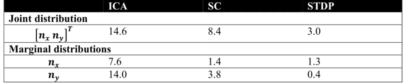
713
Kullback-Leibler divergence of receptive-field shape distributions 714 ICA SC STDP Joint distribution [𝒏𝒙 𝒏𝒚]𝑻 14.6 8.4 3.0 Marginal distributions 𝒏𝒙 7.6 1.4 1.3 𝒏𝒚 14.0 3.8 0.4 715
Table S 1: Kullback-Leibler (KL) divergence of frequency-normalised spread vectors (FSVs) from the models to 716
the macaque distribution. The receptive-field (RF) shape of the neurones from the models and measurements in 717
macaque V1 (Ringach, 2002) was parametrised by estimating the frequency-normalised spread vectors (FSVs). 718
FSVs are characterised by two parameters 𝑛𝑥 and 𝑛𝑦: 𝑛𝑥 is proportional to the number of lobes in the receptive 719
field, and 𝑛𝑦 is modulated by its elongation. The KL divergence reflects the number of additional bits required to 720
encode the parameter(s) of interest from the macaque data using the distributions from one of the three models 721
(ICA, SC or STDP). The KL divergence for the FSV reported in the Results section was based on an estimation 722
of the joint distribution of the two FSV parameters. Here, we also report the KL divergence for the marginal 723
distribution of each FSV parameter separately. All values are in bits. 724
Frequency-normalised spread vector distributions 725
726
Figure S 1: Frequency-normalised spread vector (FSV) distributions. FSVs are a compact metric for quantifying 727
RF shape. To facilitate comparison with macaque data in Figure 2D, the two axes were cut off at 1.5 (marked with 728
red, dashed lines). Here, we show the data without any cut-offs. The macaque data (black) and STDP (pink) are 729
limited to a small region near the origin, while ICA (green) and SC (blue) show a much higher range of values. 730
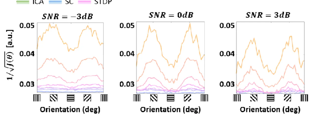
Effect of noise on ideal observer responses 732
733
Figure S 2: Ideal observer response across noise levels. Approximations of Fisher information were used to 734
estimate ideal observer responses to sine-wave gratings with additive Gaussian noise (Figure 4B). The 735
approximations were made at three noise levels: -3dB, 0dB and 3dB, corresponding to the variance of the noise 736
being double, equal to or half the signal variance. 737
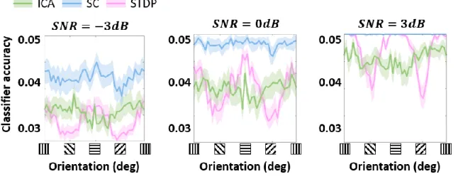
Effect of noise on linear decoding 739
740
Figure S 3: Classification accuracy across noise levels. Decoding scores of a linear classification model were 741
calculated by using stimulus orientation as the class labels and population responses to the stimuli as the 742
training/testing data (Figure 4C). The stimuli used were sine-wave gratings with three levels of additive Gaussian 743
noise: -3dB, 0dB and 3dB, corresponding to the variance of the noise being double, equal to or half the signal 744
variance. 745
Effect of noise on the cardinal orientation bias 747
748
Figure S 4: Cardinal orientation bias across noise levels. The threshold of the STDP model was increased/decreased 749
post-convergence to investigate its effect on the modulation of the ideal observer response at horizontal and vertical 750
(cardinal) orientations (Figure 4D). Oriented sine-wave gratings with additive Gaussian noise were used for these 751
simulations. The simulations were run at three noise levels: -3dB, 0dB and 3dB, corresponding to the variance of 752
the noise being double, equal to or half the signal variance. 753
Fisher information from spiking and non-spiking responses 755
756
Figure S 5: Spiking and non-spiking activity. The STDP model was presented with oriented sine-wave grating 757
stimuli (see Methods and Figure 4A) and the resulting activity was used to estimate the Fisher information using 758
spiking and non-spiking responses of the network. This was used to compute ideal-observer performance as a 759
function of the stimulus orientation. 760