Statistical and geometrical definition of snow avalanche runout

(1)

Publisher’s version / Version de l'éditeur:

Cold Regions Science and Technology, 13, 2, pp. 107-19, 1987

READ THESE TERMS AND CONDITIONS CAREFULLY BEFORE USING THIS WEBSITE. https://nrc-publications.canada.ca/eng/copyright

Vous avez des questions? Nous pouvons vous aider. Pour communiquer directement avec un auteur, consultez la première page de la revue dans laquelle son article a été publié afin de trouver ses coordonnées. Si vous n’arrivez pas à les repérer, communiquez avec nous à PublicationsArchive-ArchivesPublications@nrc-cnrc.gc.ca.

Questions? Contact the NRC Publications Archive team at

PublicationsArchive-ArchivesPublications@nrc-cnrc.gc.ca. If you wish to email the authors directly, please see the first page of the publication for their contact information.

NRC Publications Archive

Archives des publications du CNRC

This publication could be one of several versions: author’s original, accepted manuscript or the publisher’s version. / La version de cette publication peut être l’une des suivantes : la version prépublication de l’auteur, la version acceptée du manuscrit ou la version de l’éditeur.

Access and use of this website and the material on it are subject to the Terms and Conditions set forth at

Statistical and geometrical definition of snow avalanche runout

McClung, D. M.; Lied, K.

https://publications-cnrc.canada.ca/fra/droits

L’accès à ce site Web et l’utilisation de son contenu sont assujettis aux conditions présentées dans le site LISEZ CES CONDITIONS ATTENTIVEMENT AVANT D’UTILISER CE SITE WEB.

NRC Publications Record / Notice d'Archives des publications de CNRC:

https://nrc-publications.canada.ca/eng/view/object/?id=7db94ef4-cf93-4874-a484-f962213f193a https://publications-cnrc.canada.ca/fra/voir/objet/?id=7db94ef4-cf93-4874-a484-f962213f193a

(2)

Ser

TH1

N21d

no.

1460

'

c,

2 BLDG

National Research Conseil national

I+

Council Canada de recherches Can& Institute for lnstitut de

Research in recherche en Construction construction

Statistical and Geometrical Definition

of Snow Avalanche

Runout

by D.M. McClung and K. Lied

Re~rinted from

cold Regions Science and Technology Vol. 13, No. 2, 1987 p. 107-119 (IRC Paper No 1460) Price $3.50 NRCC 27715

I

I R C

CNRC

-

ICIST

I

(3)

Deux modlles mathsmatiques d e c a l c u l de l a c o u r s e maximale d'une avalanche 3 p a r t i r d ' u n p o i n t de r s f s r e n c e f i x e s u r l a t r a j e c t o i r e s o n t p r b e n t S s e t compar6s. Les modsles s o n t : ( 1 ) d e s e s t i m a t i o n s &e l i m i t e s de c o n f i a n c e concernant d e s a n a l y s e s de r e g r e s s i o n d e s p a r a d t r e s topographiques, e t ( 2 ) un c a l c u l d e s l i m i t e s de c o n f i a n c e pour d e s e s t i m a t i o n s de l a c o u r s e 3 p a r t i r de l a s t a t i e t i q u e d e s v a l e u r s extremes. En u t i l i s a n t ce d e r n i e r modsle pour d g f i n i r l a course, e t d e s approximetiona polynomtales dee p r o f i l e des t r a j e c t o i r e s d e s avalanches, on a c o n s t r u l t un modele g6omGtrique d e t e r r a i n . Eneemble, ces modkles r e d d f i n i s s e n t le problkrae c l a o s i q u e de r S p a r t i t i o n d e s zones d ' a v a l a n c h e s e n d i s t i n g u a n t : (1) une e s t i m a t i o n de l a course, n k c e s s i t a n t une d k c i s i o n t e c h n i q u e q u a n t au choix d e l a Limite de c o n f i a n c e , e t (2) un problame d y n a d q u e n S c e s e i t a n t d e s e s t i m a t i o n s d e l a viteese le long du p l a n i n c l i n E e n t r e l e a p o e i t i o n e d e d t p a r t e t d ' a r r g t , l a g k o d t r i e Qtant dSterminde p a r le m d s l e g k m s t r i q u e e n t r e cee p o s i t i o n s .

(4)

Cold Regions Science and Technology, 13 (1987) 107-1 19

Elsevier Science Publishas B.V, Amsterdam - Printed in The Netherlands

STATISTICAL AND GEOMETRICAL DEFINITION OF SNOW AVALANCHE RUNOUT

D.M. McClung

National Research Council Gnada, Vancouver, British Columbia (Canada) and K. Lied

Norwegian Geotechnical Institute, Oslo (Norwad

(Received January 9, 1986;accepted in revised form March 27, 1 9 8 6 )

ABSTRACT

Two mathematical models for calculating the ex- treme avalanche runout from a fixed reference point on the path are presented and contrasted. The models are: (1) estimates of confidence limits on regression analyses o f topographic parameters and (2) calcula- tion of confidence limits on runout estimates from ex- treme value statistics. Using the extreme value statistics model to define runout, and polynomial fits to ava- lanche path profiles, a geometrical model for ava- lanche terrain was constructed. Taken together, these models redefine the traditional zoning problem by di- viding it into ( I ) an estimation of runout distance, re- quiring an engineering decision on the choice of con- fidence limit, and ( 2 ) a dynamic problem requiring speed estimates along the incline between the start and stop positions, with the geometry specified by the geometrical model between these positions.

The engineering aspects of zoning for avalanche- prone regions may be separated into two parts: (1) estimating runout distances for the extreme event on a path based upon statistical models that include topographic features and the choice of a confidence limit selected by an engineering decision and (2) defining speeds along the incline between the start position and runout position. In this paper, the first part of the problem is introduced and examples are given that illustrate the applicability and limitations of the method. The second part of the problem is considered by defining a terrain model. This model gives to extreme runout predictions a quantitative, geometrical interpretation, thereby providing path geometry between start and stop positions in a systematic way. The terrain model should prove useful for examining the effects of varying path parameters in avalanche dynamics modelling.

INTRODUCTION DESCRIPTION OF DATA AND VARIABLES

The traditional method of determining maximum runout distances and impact .pressures of snow avalanches for zoning purposes involves predicting jointly the avalanche runout and dynamics by selecting appropriate friction coefficients for an avalanche dynamics model. The actual physical modelling required for this approach involves many unknowns including: constitutive equations, boundary con- I _{ditions and descriptive and quantitative features of} flowing snow. These gaps in knowledge are signifi- cant; clearly the problem is far from solved.

The data set used for the present analysis consists of topographic parameters for 212 avalanche paths from the maritime climate region of Western Norway. Extreme runout positions for time scales of at least 100 years were measured in the field, and additional parameters of the avalanche paths were determined. Papers by Lied and Bakkehdi (1 980) and Bakkehdi, Domaas and Lied (1983) provide basic descriptions of the parameters.

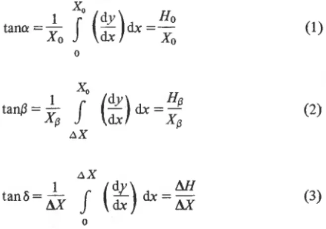
The parameters used in the present analysis are defmed in Fig. 1. The following equations provide

(5)

definitions of the first three variables, angles a ,

0,

6 measured in degrees:

The fourth variable is the starting zone angle defined by t a d , the average slope in the first 100 m of vertical drop of the avalanche starting zone. The origin of geometry is the extreme tip of the runout (a point), and the

0

point (AH, AX) is that for which the slope angle first equals 10' proceeding downslope from the avalanche start position.

The

0

point is chosen as a reference for the definition of runout, and tans is the average slope in the runout zone. Since is a zero reference point, runout distances can be regarded as taking positive or negative values if the avalanche stop position is below or above the

0

point, respectively.

For eqns. (1-3), AX and AH are the horizontal reach and vertical distance, respectively, to the

0

point and Xo and Ho are the horizontal reach and

Fig. 1. Definition of pqameters used in the analyses in relation to an avalanchepath.

vertical drop, respectively, from the start position to the runout position.

The angle a was measured in the field using a clinometer, whereas most of the values for

0,

6 and 8 were determined from maps with a scale of 1:5000 and contour intervals of 5 m. The a angles, which

-

represent an estimate of the tip of the avalanche debris based on observations of damage from the dense core of the avalanche, do not generally include the effects of powder clouds which are observed to travel much further. Errors have probably occurred when damage from the powder portion of the avalanche was mistaken for damage from the tip of avalanche debris. Most of the angles in this analysis are accurate to the nearest degree, with only a few being determined to the nearest half-degree (Bak- keh$i, Domaas and Lied, 1983).

No length parameters were measured for the present data set. However, three parameters with length dimensions were calculated from terrain profiles of the avalanche paths in the data set. These length scales were calculated by fittiqg the polynomial curve y = ax2

+

bx

+

c to the avalanche terrain profiles. It was found that this polynomial provided an excellent fit t o the avalanche terrain profiles. In most instances the correlation coefficient,R, was greater than 0.98. The three length parameters calculated were: y" = 242, H and L (Fig. 1) where H is the vertical distance from the avalanche start position to the position where y' = 0 and where L is defined as Hltana, the approximate horizontal reach of the avalanches. Calculations show that H is very close to the vertical drop of the avalanches in most instances. The values in Table 1 list some properties of the primary variables in this study. Histograms for these variables showed that most may be considered to have an approximately Gaussian distribution. Ins- pection of the value in Table 1 shows that the mean differs from the median most significantly for the variables 6, i and y". The constructed histograms showed that these variables appear to deviate the most from a Gaussian distribution. Some of the values in Table 1 are given to an accuracy greater than that of the variables they are calculated from. For d

example, the mean values and standard deviations of the angles are given in tenths of degrees. This was done for the purposes of analysis only and does not imply the angles are known with such accuracy.

(6)

TABLE 1

Primary variables in the analysis

Variable Mean Standard Median Range No. of

deviation avalanche paths

REGRESSION ANALYSIS O F TOPOGRAPHIC transformation on a. Power law regression gave a

PARAMETERS good unbiased relationship

& = O.730fl1.O6

With

/3

as a reference point from which to calculate ( 5 )

runout and a as the response variable, all the primary with R 2 = 0.861, S = 0.0764 and the F statistic variables listed in ~ a b i e 1 can qualify as piedict& = 1306. The correlation coefficient, R = 0 9 2 8 , is variables except 6 and L. The use of 6 as a predictor identical in this case to the Spearman rank correla- variable is limited to those few cases where the terrain tion coefficient, R s , which shows the curvilinear in the runout zone angle is at a constant angle. For aspect implied by the data.

the present data set, 13 1 paths have known 6 angles Another transformation explored was

6

For whereas the other primary variables are known for this case the regression equation is

212 avalanche

p he-variable

L cannot be used as a predictor because it is calculated from a knowledge of a.

Correlation coefficients ( R ) were calculated for a with respect to the other variables in Table 1, giving: 0.919 @), 0.388 (O), -0.111 (ti), 0.245 (If), -0.519 ( L ) and 0.615

0").

A dimensionless product variable ~ y " introduced by Lied and Bakkehgi

(1980) has a correlation coefficient of 0.754 with respect to both a and

8.

In this regression analysis, eKtreme runout is based upon a prediction of the minimum value of a for given values of the predictor variables. An exarnin- ation of the correlation coefficients and an optimal regression analysis showed the best one-predictor model t o be of the form a =

fC11).

Linear regression gave the following equation for all 21 2 avalanches

with R 2 = 0.845 and the standard error, S, = 2.52".

'

_{The value of the F statistic is 1148 for eqn.}_{( 4 ) .}

A plot of the residuals vs. a and

0

showed that eqn. (4) provides biased estimates. This suggested a

with R 2 = 0.853, S = 0.218 and the F statistic =

1220. Plots of residuals showed that, although this equation removes some of the bias in estimates that was found in the linear model, it is not as good in that respect as eqn. ( 5 ) . Equation ( 6 ) may prove useful in some applications.

Many other relationships were explored, including multiple regression equations. It was concluded that

8, H and y" are not useful for improving the predic- tion of a through a multiparameter relationship containing fl. Adding almost any variable to a multiple regression scheme will improve the multiple correlation coefficient and may reduce the standard error. However, extensive analyses with the present data set showed that adding predictor variables to

0

improves /I2 and the standard error only slightly, over the one-parameter models [eqns. ( 5 ) and ( 6 ) ] . In all cases explored, the resulting equations were either overfitted or the changes in prediction were not sig- nificant enough when compared with the accuracy of the input data, and consequently, inclusion of other

(7)

predictor variables was not warranted. Equations ( 5 ) and ( 6 ) explain 85-86% of the variation of a

through variations in

P,

which means that

8

has a dominating influence. .It would be very difficult to improve upon this result by adding a second variable.

Adding 6 as a predictor variable, along with

8,

slightly improves the prediction of a. In view of the geometrical connection between a,

8

and 6 (Fig. l ) , it would be surprising if this were not

sb.

Multiple regressions gave the following relations analogous to eqns. (4-6) for 13 1 avalanche paths

6 = 0.9606

+

0.222 6 - 3.18" R 2 = 0.889,s = 1.79 and F = 512 ( 7 ) = 81.04 exp[-0.296

+

0.0071861 R 2 = 0.889, S = 6.06 X and F = 514 ( 8 ) &= 0.08798

+

0.01986,+ 2.42 R 2 = 0.891, S = 0.163; and F = 522 (9)

A plot of the residuals vs. response and predictor variables showed that eqns. ( 8 ) and ( 9 ) provide good unbiased predictions. Expression ( 9 ) is the best two- predictor equation found. For eqn. (9), the t statistic for the variable

8

is 32.1 and for 6 it is 4.68. For the subset of 13 1 avalanche paths for which 6 is known, calculations show that = 0.08458

+

2.66 with

R 2 = 0.872, S = 0.1 76 and F = 880 for comparison with eqns. (6) and (9).

At attempt was made to derive better predictive equations for selected ranges of the parameters of I

the paths. For an accurate statistical analysis over the ranges of parameters in the present study, data from about 100 paths should be included. Since the present data set has 212 avalanche paths, data subsets above and below the median values of the parameters listed in Table 1 should be analyzed. Calculations for these subsets of 106 avalanche paths showed better predictive equations (in the sense that the standard errors were lower) for parameters in the range:

8 <

33", H

>

830.5 m, L

>

1342.6 m, and 9

<

41.75". Given a value of H,

8

is related to path length with lower vaiues corresponding t o longer paths. In addition, it is suspected that avalanche size and frequency is related to starting zone angle: lower starting zone angles mean larger and less frequent

avalanches. A glance at the ranges of parameters above shows consistently that the modelling is more accurate for longer paths and perhaps for larger avalanches. Equations analogous t o eqns. ( 4 - 6 ) for these data subsets were derived. The results of these calculations showed that for

0 <

33" the standard -

errors were significantly lower but the fits ( R 2 ) were not as good as for all the data. For f3

<

41.75" no improvement in fit was noted but the standard

-

error was reduced over equations for all the data. For the-106 avalanche paths with L

<

1342.6 m, the

but the standard errors were larger.

The best results were found for the parameter L greater than the median value. For L 2 1342.6 m the following results were derived analogous to eqns. (4-6) for 106 avalanche paths

For the 106 avalanche paths with L

<

1342.6 m, the following equations were derived

These analyses show consistently that the longer avalanche paths can be modelled more accurately. The parameter L seems to be the best scale of those chosen so far because it takes into account that better regression equations are available for lower

8

values and higher H values; that is, L accounts for both of these effects.

There are a number of reasons why longer paths should give better results. One reason is that errors in

(8)

determining parameters may be magnified for short paths. A second, and perhaps more likely reason, is that the position of the centre of mass of the deposit should provide a more consistent measure of runout than does the tip of the debris as used in the present

-

_{study. For the shorter paths, the length of the debris}

deposit may become comparable to length scales such as L or H. When the length of the deposit is less than

-

_{approximately 10% of L, the location of the centre of}

mass would be less important. Consultants using these models should recognize that application of the models would give runout distances too short for short avalanche paths.

Strictly speaking, L Cannot be used as a predictor variable for the present data set since it is derived from a knowledge of a. However, a two-parameter model with

0

and L shows the influence of L indicated above. Multiple regression (for 212 avalanche paths) showed

which may be compared with eqn. (5). For typical values

0

= 33" and L = 1000 m, the value of a

changes by more than 1" from eqn. (5). It appears that measured values of a horizontal reach length scale, or perhaps path length, may result in improve- ments in the regression schemes for future data sets. Equations (1 0-1 5) show the same trend as eqn. (6): given a value of

0,

increased values of L imply a lower a angles.

AN ALTERNATIVE SCHEME FOR AVALANCHE RUNOUT PREDICTION

Another method of estimating runout is to calculate the distance in metres from the

0

point to the measured runout position (a point). From eqns. (1- 3) and Fig. 1 it can be seen that

I

and similarly

For the present data set with known values for 131 avalanche paths, calculations show that M I X P has a mean value of 0.171, a standard deviation of 0.1 13 and a range of -0.121 to 0.523. The parameter

M / H P has a mean value of 0.276, a standard devi-

ation of 0.197 and a range of -0.209 to 0.969. Calculation of correlation coefficients and multiple regression analyses indicated that M I X p and AX/Hp

are statistically independent of all the predictor variables to a good approximation. Histogram plots showed that neither of these quantities are Gaussian variables.

Calculation of Spearman rank correlation coefficients, R , , showed that correlating M I X p with respect to

0

results in R , = -0.068 and correlating

M / H p with respect to results in R , = -0.332.

These coefficients differ little from the ordinary correlation coefficients (-0.061 and -0.336, respectively), but the Spearman coefficient does not employ Gaussian assumptions and is considered a better indicator. The negative correlation coefficients are consistent with the trend from the previous analysis concerning path length effects for the regression models. These and other calculations show that the assumptions of statistical independence with respect to predictor variables is better for M I X P

than for M / H P . This assumption is utilized in a model for extreme runout prediction in the next section.

STATISTICAL PREDICTION OF EXTREME AVALANCHERUNOUT

The regression models and the parameter M I X p

constitute alternatives for calculating extreme runout from the

0

point as a reference position. Both alternatives are developed in this section.

Calculation of extreme runout for the regression model depends on a prediction of minimum a.

Specifying extreme runout corresponds to extimating the upper confidence limits on the distribution of

0

(ordinate) vs. a (abscissa). For the present analysis such upper confidence curves are calculated on a point-by-point basis given values of

0.

Alternative definitions are possible (e.g. Miller, 1980). For a linear model, the upper P% value of the confidence interval for predicting a minimum value of a , with a

(9)

value of

0

= Do, is given by (Walpole and Myers, 1978)

where t(l-p/lOO) is a chosen value of the t distribution with N - 2 degrees of freedom, N is the numlier of avalanche paths, X ; is the row vector (1 Po), and Xo is the corresponding column vector. The 2 X 2 matrix A-' is the variance-covariance matrix of the estimated regression coefficients. With

a2 as the variance of the regression equation, A-' a2

has variances on the diagonal and covariances on the off-diagonal elements.

Detailed calculations have shown that for 210 degrees of freedom, eqn. (19) may be safely approxi- mated by

ap =

=

- -(l-~/100) S (20)

The correction term d l

+

X;A-'X~ causes at most a 2% change t o the multiplier t(l- S .

For models obtained by transforming the response variable a , eqns. (19) and (20) are replaced by the similar expressions, with alp and & replaced by the transformed variables. With this change, the best one- predictor runout model is provided by eqns. (5) and (20)

Similar expressions may be derived for the two- predictor model. In this case the row vector Xb

becomes (1

Do

60) and the variance-covariance matrix is a symmetric 3 X 3 matrix. The best two- predictor model is where A

-'

r0.388'7 - 1.002 X 10-'

-

8.168X I O - ~ ~ A-1 =

I

2 . 8 3 3 ~ 1 0 ~ I.l56X1O4 (symmetric) 6.736X

J

for N - 3 = 128 degrees of freedom.

Calculations at the mean values @= 32.7" and

6

= 6.5" show that d l

+

X ~ A - ' X ~ = 1.03 for the minimum correction to the approximate expression

G=

0.08790

+

0.01986

+

2.42

- [0-1631 [t(1-~/100)1 (23)

Equations (22) or (23) may be used in those restric- ted cases for which the runout zone has a constant or approximately constant known slope angle.

Equations (21) to (23) state that, given a value of

0

and a value of P between the limits 50

<

P

<

100,

P%

of avalanche paths in the data set are estimated

-

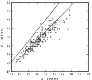
t o have a angles greater than c+. For the number of degrees of freedom in the data set, the t distribution is nearly indistinguishable from a Gaussian distribution. Calculations with P = 99 and P = 50 for which to. o l = 2.326 and to. = 0.0, are illustrated in Fig. 2 for eqn. (21).

The alternative to predicting runout using the regression model is to specify M I X p for long-running avalanches. Since this parameter is statistically

;

independent of 0, 8 and 6 to a very good approximation, values could be extrapolated beyond the mean value, independent of these parameters. The ratio M I X p is not a Gaussian variable; therefore, several other distributions were tried, including log- normal, Weibull and extreme value (Gumbel). It was found that the best model is provided by the first asymptotic extreme value distribution (Chow, 1964).

a , d e g r e e s

Fig. 2. Prediction of values of a for P = 50 and P = 90 for the

regression model [eqn. (21)l. Extreme runout corresponds

to the upper envelope of the data points when 0 (ordinate)

I

is plotted vs. a (abscissa). The 212 avalanche paths are

represented by (A) with some points representing multiple

(10)

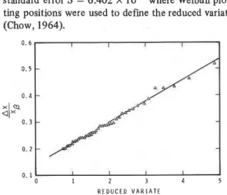
The fit of the extreme values of AX/Xp to this distribution is nearly perfect. The 50 highest values of AX/ Xp are plotted on extreme value probability paper in Fig. 3. Regression analysis of M I X p with the reduced variate -ln[-ln(P/100)] gave R' = 0.993 with a standard error S = 6.402 X 10-3 where Weibull plotting positions were used to define the reduced variate (Chow, 1964).

R E D U C E D V A R I A T E

Fig. 3. Plot of AXIXp vs. the reduced variate for the 50

highest values of runout on extreme value probability paper using Weibull plotting positions.

The extreme value distribution gives the model

where 50

<

P

<

100. The choice of P = 50 gives a mean value of 0.171. Equation (24) states that

P%

of avalanche paths in the data set (1 31 paths) have a horizontal reach less than (AX/XP)p. For P = 50 and P = 99, the values predicted in eqn. (24) are 0.171 and 0.509, respectively, which may be compared with the Gaussian predictions of 0.171 and 0.434. The fact that the highest values of avalanche runout appear to obey extreme value statistics is not particularly surprising. Extreme value distributions are known to characterize flood data in hydrology work, and the physical analogy to extreme, avalanche events seems reasonable.

The regression models and the extreme value model constitute alternative mathematical prediction

r schemes for extreme runout based on the data set. Specific applications may require one or the 0th-

Experience indicates that the models are largely equivalent to within data accuracy.

Equations (21 -24) may help to provide a mapping for extreme runout distances in zoning applications. The value of P in these equations is determined by a decision of the acceptable risk, based upon the value and use of the land and upon the desired level of safety, conditioned by the estimated return period for the climate regime in question. In many instances where land prices are high, P = 99 would provide unacceptable runout predictions because the very long distances implied would exclude much expensive land from consideration for construction.

More importantly, eqns. (21-24) provide a mathematical framework to examine measured runout on avalanche paths, in order to defme those with an exceptionally long reach. Close examination of those paths with long runout may reveal patterns in terrain features that can provide a basis for more accurate runout prediction and zoning models in the future. Studies of avalanche paths outside the present data set have defined several types of avalanche terrain profiles that produce excessively long runout. Some examples are given in a later section.

GEOMETRICAL DEFINITION OF RUNOUT The runout models defined thus far are derived from angles with no particular geometry implied. In this section, predicted avalanche runout is interpreted in terms of aperrain model that provides a geometri- cal definition.. A geometrical model may be useful for future avalanche dynamics modelling; in addition, it gives a pictorial representation of the runout prediction models.

Regression analysis for the avalanche paths in the present study has shown that when the terrain profile is plotted with heights, y, versus horizontal distances, x, the polynomial y = ax2

+

bx

+

c gives an excellent fit to the terrain. In the great major@ of cases, R

>

0.98 and additional terms are unnecessary to accurately describe the terrain. The terrain model given in this paper consists of defming a, b and c in terms of a,

0

and 6 for a given confidence limit or value of P.

In defining the actual runout position in the terrain model, two different assumptions were em- ployed: (1) the regression model given by eqn. (21); and (2) the prediction of maximum runout from extreme value statistics given by eqn. (24). Analyses

(11)

using these models showed that the latter model is preferable. For a given value of 0, the extreme value statistics model gives a terrain model with runout distances that are consistent with the regression model predictions within data accuracy.

Fbr the polynomial y = ax2

+

bx

+

c, the origin is chosen at the tip of the runout. In the present data set, the avalanches either stop above the valley floor or they run out onto a flat valley floor. Those avalanches that run up the opposite mountainside were ex- cluded. Thus, the terrain model utilizes the polynomial expression for avalanches that do not reach the valley floor and a combination of the polynomial expression and a level straight-line segment for those avalanches that do reach the valley floor.

With the chosen origin of coordinates, the additive constant c in the polynomial may be ignored. The slope at the origin is: dy/dxlo = b ; this quantity is zero for avalanches that reach the valley floor. The parameter tan6 defines the average slope in the runout zone from the

0

point to the origin. For tan6

>

d,tanloO, the stop position is at or above the valley floor. For tan6

<

itanloo, b = 0, which suggests the use of the parabola y = aw2 and a straight line segment as the terrain model for these values of 6.

For the polynomial y = ax2

+

bx

+

c (6

>

5.044

tan6 = tana - tar$

+

tanlO0 ₍₂₅₎

For a runout position just at the valley floor, tan6 =

3tan1O0, which suggests a definition of an angle a' such that tana' = tan0

-

itanloo where a' defines the position of the valley floor. For the patabola y

= ax2, a = t a n 2 a ' / ~ , where H is the vertical drop from start position to the valley floor. Similarly, it may be verified that

H

- -

-

2tan2 a' _{or, with tan/3}₌

_-

Hl3

Hg

tanp(2tana1

-

tanlO0)

x~

This last expression becomes

The horizontal reach from the

0

point to the valley dloor, AX', is given by

The runout position (AX/Xp)p is given by eqn.

1

(24). The length of a straight line segment, AXo,

for P values that imply an avalanche reach beyond the valley floor (6 G 5.04') is obtained as follows

(28)

For avalanches that reach the valley floor and beyond (6

<

5.044, , the average slope in the runout

zone is (from eqns. (1 7) and (24))

Similarly, the a angle is defined by

For avalanches that do not reach the valley floor (6

>

5.04'), the polynomial y = ax2

+

bx is used with the origin at the runout position. From eqns. (17), (24) and (25) it is easily shown that

and similarly

Using dy/dxlAX = 2 a ( W

+

b and eqn. (17), the parameter b is denved to be

For 6

>

5.04', a x p is given also by eqn. (26).

Another quantity of interest is the path length,

Sp, along the polynomial y = ax2

+

bx

+

c from the starting position t o the 10" point on the path. Inte- gration gives the following ratio

where 80, the initial angle on the curve, is tan@. =

(12)

Equations (25-33) defme a complete system of equations for a geometrical terrain model, given chosen values of

0

and P and a length scale Xp or Hp with the runout position defmed by extreme value statistics. These equations define avalanche terrain in

-

a systematic way consistent with measured data on

.

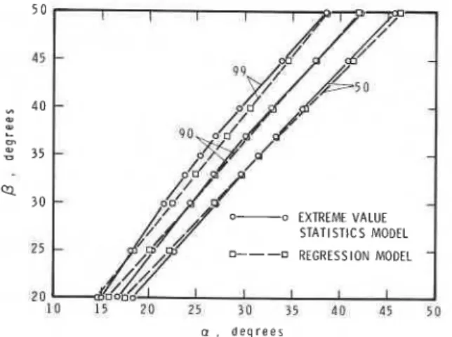
avalanche runout and terrain profile fits to actual avalanche paths. llus terrain profile model may be of use in theoretical avalanche dynamics modelling. It will enable realistic values of terrain parameters to be introduced in an organized manner in studies of the application of the model to real situations.

It is of interest that the predictions of ap from the terrain model are in good agreement with the one- parameter regression model described by eqn. (21). Figure 4 shows a comparison for 99%, 90% and 50% confidence limits. The differences are greater at the highest confidence limits, but they are generally less than l o , which corresponds to data accuracy in the present study.

The regression model was used as an alternative to define the runout position for a different terrain model. Calculations showed that predicted runout exceeded that obtained from extreme value statistics for high values of P. This supports the choice of the extreme value statistics model for runout defmition in the terrain model. This seemingly paradoxical result is due to a slight mathematical differences in the two runout models.

5 0 45 4 0 3 5 3 0 o EXTREME VALUE STAT1 STlCS MODEL

25 _n---o _{REGRESSION MODEL}

1 0

10 1 5 PO 25 3 0 3 5 4 D 4 5 5 0

a , d e g r e e s

Fig. 4. Comparison of runout predictions for the two statis- tical runout models as a function of confidence limit (P value). The extreme value statistics model is used to define runout positions for the terrain model. These positions are used to calculate values of ap for comparison.

The terrain model implies some interesting charac- teristics of runout which may or may not be correct. Since (AX/Xp)p is independent of

0

in the model, from eqn. (34) the ratio of path lengths for ( X p

= constant)

0

= 20" and

0

= 50" is S201S50 = 0.665. The implication is that AX20/AX50 cz $ ( s ~ ~ / s ~ ~ ) ,

independent of the confidence limit. For Hp = constant, Szo = 2.937 Hp and S S 0 = 1.348 Hp, or equiva- lently, AX20 = 3.27 AXso. The result indicates a strong path-length dependence. One possible physical interpretation is that rapid deceleration does not begin until the slope angle reaches nearly lo0, causing longer runout. These path-length effects are similar to, but much stronger than those shown for the regression models [e.g. eqn. (16)l.

Path-length effects are shown (Hp scaled to unity) for the terrain model in Fig. 5 using the 99% confidence limit with /3 = 20", 33" and 50". This figure also illustrates another feature of the terrain model: the maximum reach onto the valley floor is predicted for

0

angles, which depend on the confidence limit chosen. From eqn. (28), the angle, fim,,, which produces the maximum distance onto the valley floor, is defined by

where y = tan10~-[[2(AX/AX~)~

+

I ] /(AX/AXP)p). For P = 99, this gives

PmaX

= 30.8"; for P = 90,

omax

= 38.8"; and for P = 60,

Omax

= 52.2". These results are a mathematical feature of the model chosen, and are a consequence of the choice of origin and the polynomial curves.

Fig. 5. Illustration of profiles of y versus x predicted by the terrain model for P = 99. The solid lines (-) connect the start position and the p point, The dashed lines (--) connect the start position and the or' point. Points on the predicted profdes are denoted by: (o, p = 20') (0, p = 33') (A, p =

(13)

By inspection, Fig. 5 also shows that for Hp =

constant, a profile with

0 =

20" implies a value of AX, more than three times as large as for a profile with

0

= SO", which is why Lied and Bakkeh4i (1980) consider profiles with low values of to be of great importance in land use planning. Prime building land normally has slope angles below 10".

EXAMPLES OF RUNOUT CALCULATIONS FOR EXCEPTIONALLY LONG RUNOUT

In this section, sample runout calculations are given for avalanches outside the present data set t o illustrate predictions, limitations and problems of the modelling.

An interesting example is the Salezertobel avalanche in Switzerland discussed by Fohn and Meister (1981). These authors showed that runout distances based upon the tip of the debris from the extreme event for each year appear t o obey extreme value statistics in direct analogy to flood data from hydro-

I

R E A C H , m -5

4 I I 1 I I 1 1 I l l ' 1 9

2 - ALL EXTREME NCNTS PER YEAR lSALEZERlOBELl 0

-

19Ml37 - 8WS1 8

-

6

-

4

-

Z a L I l l ) h 1.01 1.1 1.5 2 3 4 5 10 20 30 50 100 200 M E A N R E T U R N P E R I O D , y e a r s

Fig. 6. (top): The Salezertobel avalanche profile. (bottom): Comparison of predictions of the regression model (0) and the extreme value statistics model (0) plotted on the extreme

value statistics line calculated by Fohn and Meister (1981) for runout distance (9 vs. mean return period.

ogy. For this path, Xp = 1770 m, Hp = 855 m and

0

= 25 .go. The calculations of Fohn and Meister show that measured runout has a good correlation (lZ2 =

0.936) with respect t o the reduced variate of the extreme value distribution for the longest running event for each year (46 years data). They defined

-

runout (S) as the horizontal distance from 395 m

-

before the

0

point. Figure 6 shows measured runout

-

on the path, and the predictions of runout from the regression model (eqn. 21) and the extreme value statistics model (eqn. 24) for P = 50, 90 and 99. These calculations indicate implied return periods of 17-24 years for P

-

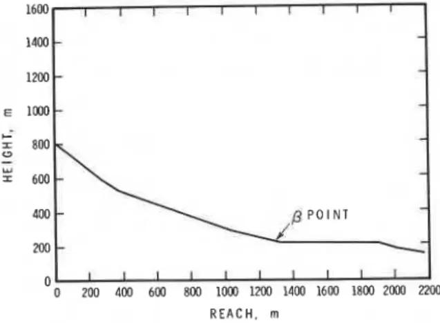
50, 60-70 years for P = 90, and 160-200 years for P = 99 for the Salezertobel avalanche. The data indicate that Salezertobel is a potentially long-running avalanche compared with the Norwegian data set. For a return period of about 100 years, the implied value of P is close to 95. These calculations imply some consistency in the modelling for the Salezertobel avalanche.

The remainder of the examples in this paper are chosen because they constitute cases which are troublesome with respect to the predictive equations. These examples may be regarded as worst cases. An example from Colorado, Ruby Peak, (depicted in Fig.7) was provided to the authors by A.I. Mears (personal communication). In this profile AX = 855 m, Xp = 13 1 5 m, a = 16.7" and

0 =

23 .go. Calcula- tions using the regression model give a99 = 17.6'; using the extreme value statistics model yields (AX/ Xp)99 = 0.509 vs. a measured value of 0.651. For the extreme value statistics model (AX/XP)99.9 = 0.693,

0

0 200 400 600 800 1000 1200 1400 1600 1800 2WO 2200 R E A C H , m

(14)

making this avalanche comparable to the one avalanche in a thousand based on the data set. There are two possible reasons for the unusual runout of this avalanche. In this profile, the terrain steepens again to a segment with a 22" slope after reaching the

0

point, potentially giving t o the debris a velocity boost resulting in added runout. Special problems for runout calculations may result from profiles with multiple

0

points; for example, when a flat or gently sloping bench occurs high on an avalanche path. This condition would not suffice t o define a

0

point. The definition of the

/3

point implies that it is reached by a monotonic decrease in slope angle proceeding downslope from the start$g zone.

Another problem with avalanche paths in a continental climate, such as Ruby Peak, is that the maximum extent of runout identified by vegetation damage may be due to the powder portion of the avalanche rather than the tip of the debris from the core of the avalanche. This can result in runout being overestimated when compared with the current data set. It may not be possible to describe avalanches from regions with a continental climate, such as Ruby Peak, using the mathematical models developed from the present maritime data set. On the other hand, the 100-year avalanche predicted by the model may have a higher probability of occurring in regions with dry snow avalanches, such as those with a continental climate. It may well be that the return period for avalanches producing the same runout distance is shorter under continental climatic conditions.

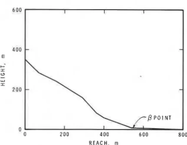
Another avalanche that is difficult to model is the Ironton Park avalanche from Colorado (Fig. 8), described by Lang, Dawson and Martinelli (1979). For this path, AX = 265 m; Xp = 550 m, and

0

=

32.5". Calculations using the runout models show that a99 = 24.5" and (AX/Xp)99 = 0.509 vs. the measured values of 24" and 0.482, respectively. These values show that Ironton Park has a long runout distance based on the criteria used in this paper. Two related reasons may explain the length of the runout. Firstly, the profile has a fairly abrupt transition at the valley floor. If the profile is steep until the valley floor has been reached, energy-absorbing, particle- locking effects may be delayed, producing longer runout. Secondly, the vertical fall and length of the path are near the minimum in the Norwegian data set. In this case the difference between the position

R E A C H , rn

Fig. 8. Profde of the Ironton Park avalanche from Colorado.

of the center of mass and the tip of the debris may be substantial relative to vertical drop or horizontal reach. This effect has been evident in several other examples (not given in the present paper) with a vertical drop less than the lower limit in the present data set (350 m). These examples have shown excessively long runout compared with predictions for the present data set.

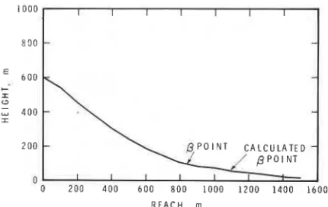
Yet another troublesome example is the Ariefa-2 avalanche (Fig. 9) reported by Frutiger (1980) and Buser and Frutiger (1980). The profile has a vertical fall of 550 m. The

0

angle estimated from the profile is 31.4" and the a angle is 20.8". The ratio M I X p is 0.896 based on the profile. These values fall outside the predictions of the regression model and the extreme value statistics model for the one-in-one- hundred avalanche. The polynomial y = ax2

+

bx

+

c

shows an excellent fit ( R ~ = 0.996) to the profile. Calculating the

0

point along the curve using dyldx

= tanloo gives an estimated angle of 27.2". Using the regression model with this figure gives ag9 =

20.7", whereas the implied value of (MIXP) is 0.442, which is near P = 98 for the extreme value statistics model. This example indicates that a

0

point defined by a polynomial fit to the profile may be a very consistent method of definition. In practice, it is suggested that a polynomial fit should be made to the profile, from which the

/3

point can then be calculated. A comparison of the calculated

0

point with that determined from the profile can indicate a troublesome profile with respect to the proposed model.

(15)

R E A C H , rn

Fig. 9. Profile of the Ariefa-2 avalanche from Switzerland showing the true @ point and another 0 point calculated by

fitting the polynomial y = ax'

+

bx

+

c to the profile. For most profiles the calculated and measured values of are very similar. For instance, the Ironton Park and Ruby Peak avalanches have calculated

0

points within a few tenths of degrees of those estimated from the profile. For the Ariefa-2 avalanche the difference is close to 4O, which is the worst example found so far. The Ariefa-2 avalanche is an interesting case because casual inspection of the profile does not reveal it as troublesome. It is indeed an avalanche path with a long runout distance, but still appears explainable as the one-in-fifty avalanche from the point of view of the extreme value statistics modelling.

DISCUSSION AND CONCLUSION

Alternative methods for calculating snowava- lanche runout distances have been presented based upon statistical analyses of a data set from Western Norway. These models are: (1) a regression analysis based upon the relation between the Gaussian variables a and /3 and (2) predictions of extreme value statistics based upon the non-Gaussian variable M I X p . The models are largely equivalent to within data accuracy.

One immediate use of the model predictions is apparent: the statistical mapping of runout distances given a value of

0

for the path, and a selection of values of P based on acceptable risk, avalanche return period and land prices at the location. In view of the uncertainties involved, it seems far more

rational to specify such a mapping of runout distances for a location rather than two distinct lines that define precisely the limits between safe areas and areas with restrictions on construction. This latter method is the most common way of specifying zones and is in contrast to that suggested in the present paper. The approach presented here is more consistent with modern engineering practice.

In most cases, the definition of values of P at a given location will be based somewhat on guesswork due to lack of data for the climate and other factors at proposed new building sites. A balance between risk and land value has to be carefully considered. Selecting a value P = 99 (the one-inane-hundred avalanche path) may result in unacceptably long runout distances in many areas where land is expensive but the risk of damage would be fairly low.

A second, more tangible, use of the runout distance models is to provide a mathematical framework for defining avalanches with long runout distances with respect to a fxed reference point. This makes it possible to focus study on extreme or troublesome avalanches to refine runout distance estimates. The three examples given in the present paper dustrate such a procedure.

Given the runout distance, or values of

p,

P and a length scale (e.g. Xp), a geometrical model for snow avalanche terrain has been given based upon polynomial fits to actual profiles. This model provides a beginning to the second part of the engineering zoning question: specifying speeds along the profile between avalanche start and stop positions. The terrain model may enable definition of avalanche terrain in a rational manner that will allow the avalanche dynamics problem to be explored theoreti- cally for variations in terrain features.

The two-part method suggested in the present paper with respect to the engineering zoning problem is in contrast to the traditional method. The traditional method is based upon selected friction coefficients in a dynamics model which are used to calculate speed estimates and runout distances simul- taneously. Such calculations are not rational at the present time because of the unknowns regarding constitutive equations and boundary conditions for flowing snow, as well as criteria for effects such as locking and snow particle break-up during collisions. Math- ematical description of such behaviour is not close

(16)

to being achieved with the accuracy required in modem zoning problems. The present paper repre- sents a proposal to divide this complicated problem into parts which are more manageable.

Several checks and refinements must be made in future studies to improve runout distance calculations. The runout models are based upon data for time scales of at least 100 years. As such, the data should represent runout from large, dry snow avalanches whereas the data set used in this paper is from a maritime climate. It is essential to compare a data set from a continental climate with the present data set.

In the present paper some possible refinements have been pointed out in regard to the modelling. One particular need for future study is the analysis of short avalanche paths with a vertical drop less than 350 m. Although these occur very frequently, no studies exist at present that can be applied to them. This illustrates the need for modelling based on sound physical principles. Field experience clearly shows that other parameters such as starting zone size, and perhaps path length, have an influence on avalanche runout distance, but explicit appearance of these effects in modelling has yet to take place.

ACKNOWLEDGEMENTS

Discussions with, and data provided, by A.I. Mears and M. Martinelli, Jr. proved very useful with regard to the examples used in this paper. This paper is a

joint contribution from the Division of Building Research, National Research Council of Canada and the Norwegian Geotechnical Institute.

REFERENCES

Bakkehbi, S., Domaas, U. and Lied, K. (1983). Calculation of snow avalanche runout. Ann. Glaciol., 4: 24-29.

Buser, 0. and Frutiger, H. (1980). Observed maximum runout distance of snow avalanches and the determination of the friction coefficients p and &. J. Glaciol., 26(94): 121-130.

Chow, Ven Te (1964). Handbook of Applied Hydrology. McGraw-Hill Book Company, New York.

Fohn, P.M.B. and Meister, R. (1981). Determination of avalanche magnitude and frequency by direct observations and/or with the aid of indirect snowcover data. Mitt. Fortl. Bundes-Versuchsanst. Wien, 144: 207-228. Frutiger, H. (1980). Ueber maximale Auslaufstrecken von

Lawinen und die Bestimmung der Reibungsbeiwerte. Interner Bericht des Eidg. Institutes fiir Schnee- und Lawinenforschung, Nr. 578, Davos, Switzerland.

Lang, T.E., Dawson, K.L. and Martinelli, Jr., M. (1979). Numerical simulation of snow avalanche flow. Research Paper RM-205, U.S.D.A. Rocky Mountain Range and Experiment Station, Fort Colliis, CO.

Lied, K. and Bakkehbi, S. (1980). Empirical calculations of snow-avalanche run-out based on topographic parameters. J. Glaciol., 26(94): 165-177.

Miller, R.G. Jr. (1980). Simultaneous Statistical Inference, 2nd edn. Springer-Verlag, New York.

Walpole, R.E. and Myers, R.H. (1978). Probability and Statistics for Engineers and Scientists, 2nd edn. MacMillan Publishing Co. Inc., New York.

(17)

T h i s paper i s being d i s t r i b u t e d i n r e p r i n t form by t h e I n s t i t u t e f o r Research i n C o n s t r u c t i o n . A l i s t of b u i l d i n g p r a c t i c e and r e s e a r c h p u b l i c a t i o n s a v a i l a b l e from t h e I n s t i t u t e may be obtained by w r i t i n g t o t h e P u b l i c a t i o n s S e c t i o n , I n s t i t u t e f o r Research i n C o n s t r u c t i o n , N a t i o n a l Research C o u n c i l of Canada, O t t a w a , O n t a r i o , K1A 0R6.

Cb document e s t d i s t r i b u 6 sous forme de t i r 6 - 8 - p a r t p a r l l I n s t i t u t de recherche e n c o n s t r u c t i o n . On peut o b t e n i r une l i s t e d e s p u b l i c a t i o n s de l l I n s t i t u t p o r t a n t s u r les t e c h n i q u e s ou les recherches e n m a t i e r e d e batiment en Bcrivant Zi l a S e c t i o n d e s p u b l i c a t i o n s , I n s t i t u t de recherche en c o n s t r u c t i o n , C o n s e i l n a t i o n a l d e r e c h e r c h e s du Canada, Ottawa ( O n t a r i o ) ,